Nonlinear Dynamic Inverse Solution of the Diffusion Problem Based on Krylov Subspace Methods with Spatiotemporal Constraints ^†

Abstract

In this work, we propose a nonlinear dynamic inverse solution to the diffusion problem based on Krylov Subspace Methods with spatiotemporal constraints. The proposed approach is applied by considering, as a forward problem, a 1D diffusion problem with a nonlinear diffusion model. The dynamic inverse problem solution is obtained by considering a cost function with spatiotemporal constraints, where the Krylov subspace method named the Generalized Minimal Residual method is applied by considering a linearized diffusion model and spatiotemporal constraints. In addition, a Jacobian-based preconditioner is used to improve the convergence of the inverse solution. The proposed approach is evaluated under noise conditions by considering the reconstruction error and the relative residual error. It can be seen that the performance of the proposed approach is better when used with the preconditioner for the nonlinear diffusion model under noise conditions in comparison with the system without the preconditioner.

1. Introduction

Krylov subspace methods are widely utilized to solve inverse problems; in particular, they are often combined with efficient preconditioners to accelerate convergence. These methods are especially effective for problems governed by parabolic partial differential equations, such as the diffusion equation, which is discretized using the finite element method (FEM).

Several recent works illustrate advancements in the use of preconditioned Krylov methods for inverse and parameterized PDE problems. For example, the authors of Ref. [1] propose a preconditioned Krylov iterative approach for an inverse source problem based on a regularized Levenberg–Marquardt method integrated with the Dual Reciprocity Boundary Element Method (LM-DRBEM). Their method addresses ill-posedness by embedding regularization directly into the iterative process. Ref. [2] introduces a hybrid preconditioning framework using DeepONet to solve parametric systems of equations. This method significantly improves the performance of Krylov solvers by preconditioning based on learned operator features. In Ref. [3], the authors develop a sine transform-based preconditioner for inverse source problems governed by time–space fractional diffusion equations. Their spectral approach improves the conditioning of the resulting matrices and enhances solver efficiency. Ref. [4] presents iterative regularization methods that can be used to solve several linear inverse problems, like the diffusion problem. However, all the analyzed cases are linear.

Most of the existing methods focus primarily on spatial discretization and overlook temporal dynamics. The explicit incorporation of temporal regularization or constraint structures into preconditioners for dynamic inverse problems is still underexplored. In addition, existing preconditioning techniques primarily address linear PDEs. However, many real-world problems involve nonlinear diffusion behavior, requiring robust nonlinear preconditioners or adaptive strategies. In this work, we propose a nonlinear dynamic inverse solution of the diffusion problem based on Krylov subspace methods with spatiotemporal constraints. The proposed approach is applied by considering, as a forward problem, a 1D diffusion problem with a nonlinear diffusion model. The dynamic inverse problem solution is obtained by considering a cost function with spatiotemporal constraints, where the Krylov subspace method Generalized Minimal Residual is applied by considering a linearized diffusion model and spatiotemporal constraints. In addition, a Jacobian-based preconditioner is used to improve the convergence of the inverse solution. The proposed approach is evaluated under noise conditions by considering the reconstruction error and the relative residual error. It can be seen that the performance of the proposed approach is better when used with the preconditioner for the nonlinear diffusion model. The work is organized as follows: In Section 2, we present the theoretical framework for the nonlinear diffusion model (forward problem) and the dynamic inverse problem with spatiotemporal constraints. The same section also presents the design of a preconditioner. In Section 3, we present the numerical results by considering a nonlinear diffusion coefficient and, in Section 4, we present the conclusions and future works.

2. Theoretical Framework

2.1. Nonlinear Diffusion Model (Forward Problem)

The forward model is defined by a 1D nonlinear diffusion equation, as follows:

$$\begin{array}{c}\hfill {\displaystyle \frac{\partial u(x,t)}{\partial t}}=\nabla ·\left(\alpha (u(x,t))\nabla u(x,t)\right)+f(x,t),\end{array}$$

(1)

where

• $u(x,t)$ is the unknown solution which is spatial ($x\in \mathsf{\Omega }$) and time-dependent (t in $[0,T]$).
• $\alpha (u(x,t))$ is a nonlinear diffusion coefficient that depends on the solution.
• $f(x,t)$ is the external input.

For a discrete-time formulation, we discretize the spatial domain $\mathsf{\Omega }$ using a mesh, and time $[0,T]$ is separated into time steps $t_0,t_1,\dots ,t_N$ with a step size of $\Delta t$. The nonlinear diffusion equation becomes

$$\begin{array}{c}\hfill {\displaystyle \frac{u_i^{n+1}-u_i^n}{\Delta t}}=\nabla ·\left(\alpha (u_i^n)\nabla u_i^n\right),\end{array}$$

(2)

where $u_i^n$ is the solution at time $t_n$ and spatial point $x_i$. This can be rewritten as follows:

$$\begin{array}{c}\hfill u_i^{n+1}=u_i^n+\Delta t\left(\nabla ·\left(\alpha (u_i^n)\nabla u_i^n\right)\right)\end{array}$$

(3)

2.2. Dynamic Inverse Problem with Spatiotemporal Constraints

The forward problem maps $u_0$ to the solution $u_T$ at time $t=T$, and the inverse problem is then used to reconstruct the initial condition from $u_T$, as described in [5]. In this case, the observed data $d_i^n$ is defined as

$$\begin{array}{c}\hfill d_i^n=u_i^n+\eta \end{array}$$

(4)

being $\eta$ the additive Gaussian noise.

In order to include spatiotemporal constraints in the solution, the following cost function is considered:

$$\begin{array}{c}\hfill J(u)=\sum _{n=1}^N\sum _i{\left(u_i^n-d_i^n\right)}^2+{\lambda }_1\sum _{n=1}^N\sum _i{\left(\nabla ·\left(\alpha (u_i^n)\nabla u_i^n\right)+f_i^n\right)}^2+{\lambda }_2\sum _{n=1}^N\sum _i{\left({\displaystyle \frac{u_i^{n+1}-u_i^n}{\Delta t}}\right)}^2,\end{array}$$

(5)

where

• The first term represents the data misfit, measuring the difference between the model’s output at each time step and the observed data.
• The second term regularizes the diffusion process, penalizing large gradients in the spatial solution.
• The third term enforces temporal smoothness, penalizing large variations between successive time steps.

The inverse problem is solved by minimizing the cost function subject to the forward model constraints and initial and boundary conditions. In addition, the nonlinear model can be approximated at each time step using a first-order Taylor expansion. Therefore, the resulting linear systems can be solved iteratively using Krylov subspace methods such as Generalized Minimal Residual (GMRES).

2.2.1. Linearization of the Nonlinear System

To solve this equation iteratively, we linearize the nonlinear term $\alpha (u_i^n)\nabla u_i^n$ by performing a first-order Taylor expansion around an initial guess $u_i^{n,k}$, as follows:

$$\begin{array}{c}\hfill u_i^{n+1}=u_i^n+\Delta t\left(\nabla ·\left(\left(\alpha (u_i^{n,k})+{\displaystyle \frac{d\alpha }{du}}{|}_{u_i^{n,k}}(u_i^n-u_i^{n,k})\right)\nabla u_i^n\right)+f_i^n\right).\end{array}$$

(6)

This is the linearized system that we need to solve for $u_i^{n+1}$.

2.2.2. Krylov Subspace Methods

Krylov subspace methods, such as GMRES (Generalized Minimal Residual) or BiCGSTAB (Biconjugate Gradient Stabilized), are employed to solve the linearized system iteratively. These methods construct a sequence of approximations to the solution by projecting the problem onto a subspace spanned by the successive powers of the matrix A (or the matrix–vector products).

The linear system can be written as follows:

$$A{u}^{n+1}=b,$$

(7)

where

• A represents the linearized operator (which includes the spatial discretization of the nonlinear diffusion term).
• $u^{n+1}$ is the vector of unknowns at the next time step.
• b represents the right-hand side (including $u_i^n$, $f_i^n$, and boundary terms).

Krylov subspace methods provide an iterative approach to solving this linear system.

2.3. Preconditioning the Krylov Method

Preconditioning is essential for improving the convergence of Krylov subspace methods. A preconditioner M is applied to the system, transforming it into a form that is easier to solve iteratively. The preconditioned system becomes

$$M^{-1}A{u}^{n+1}=M^{-1}b.$$

(8)

In general, preconditioning modifies the spectral properties of the matrix A, reducing the condition number and speeding up the convergence of the iterative solver. Common preconditioners include Incomplete LU factorization (ILU), Algebraic Multigrid (AMG) and Diagonal preconditioners, where in all cases, the preconditioner is derived from the linearized system [6].

In this work, we describe a preconditioner that approximates the Jacobian as a diagonal matrix, where the diagonal entries are based on the linearized model, as proposed in [7].

For the linearized model, we approximate the Jacobian as

$$\begin{array}{c}\hfill J=\left(\begin{array}{ccccc}{\displaystyle \frac{1}{\Delta t}}+{\displaystyle \frac{D^{\prime }(u_1)}{\Delta x^2}}& -{\displaystyle \frac{D^{\prime }(u_1)}{\Delta x^2}}& 0& \dots & 0\\ -{\displaystyle \frac{D^{\prime }(u_2)}{\Delta x^2}}& {\displaystyle \frac{1}{\Delta t}}+{\displaystyle \frac{D^{\prime }(u_2)}{\Delta x^2}}& -{\displaystyle \frac{D^{\prime }(u_2)}{\Delta x^2}}& \dots & 0\\ 0& -{\displaystyle \frac{D^{\prime }(u_3)}{\Delta x^2}}& {\displaystyle \frac{1}{\Delta t}}+{\displaystyle \frac{D^{\prime }(u_3)}{\Delta x^2}}& \dots & 0\\ ⋮& ⋮& ⋮& \ddots & ⋮\\ 0& 0& 0& \dots & {\displaystyle \frac{1}{\Delta t}}+{\displaystyle \frac{D^{\prime }(u_n)}{\Delta x^2}}\end{array}\right)\end{array}$$

(9)

where $D^{\prime }(u_k)$ is the derivative of $\alpha (u)$ at the current solution $u_k$, and where the diagonal preconditioner can be approximated as

$$\begin{array}{c}\hfill J_k={\displaystyle \frac{1}{\Delta t}}+{\displaystyle \frac{D^{\prime }(u_k)}{\Delta x^2}}\end{array}$$

(10)

3. Results

In order to evaluate the proposed approach, the forward problem of the nonlinear diffusion equation indiscrete time is defined as

$$\begin{array}{c}\hfill u_i^{n+1}=u_i^n+\Delta t\left(\nabla ·\left(\alpha (u_i^n)\nabla u_i^n\right)\right)\end{array}$$

(11)

which is the nonlinear diffusion coefficient of the form

$$\begin{array}{c}\hfill \alpha (u)=u^2\end{array}$$

(12)

but this can be generalized to other forms based on the specific problem. We discretize the spatial domain into $N_x=100$ grid points, and the time domain into $N_t=500$ time steps. The spatial step size is denoted by $\Delta x$, and the time step size is $\Delta t$. Let $u_i^n$ represent the solution at the i-th spatial point at the n-th time step, where $i=1,2,\dots ,N_x$ and $n=1,2,\dots ,N_t$. The equation is discretized using a finite difference scheme for both space and time. The Boundary conditions (Dirichlet boundary conditions for simplicity) are selected as $u(0,t)=0$ (left boundary) and $u(L,t)=0$ (right boundary), with $L=10$, and total time $T=1$.

We implement the simulation using a simple forward Euler time-stepping method for the nonlinear diffusion equation. The solution is updated at each time step based on the spatial second derivative and the nonlinear diffusion coefficient. The initial condition is defined as a Gaussian distribution, as follows:

$$\begin{array}{c}\hfill u_0=exp(-({(x-L/2)}^2)/0.1);\end{array}$$

(13)

Based on the Jacobian (9), the preconditioner can be approximated as (10)

$$\begin{array}{c}\hfill J_k={\displaystyle \frac{1}{\Delta t}}+{\displaystyle \frac{D^{\prime }(u_k)}{\Delta x^2}}\end{array}$$

(14)

with $D^{\prime }(u_k)$ being the derivative of the diffusion term (12).

Two cases are considered with a noise $\eta =0.005$ and noise $\eta =0.05$. Figure 1 depicts the simulation data.

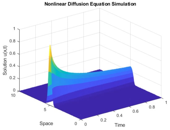
Figure 1. Simulation with noise given by $\eta =0.005$.

It can be seen from Figure 1 that the initial value at time $t=0$ is given by (13). In addition, it is worth noting that the z-axis is directly related to the colour of the surface.

Figure 2, the estimation data is shown using the preconditioner described in (14).

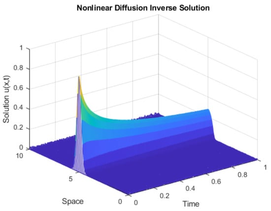
Figure 2. Estimation with a noise given by $\eta =0.005$ and with the preconditioner of (14).

It can be seen from Figure 1 and Figure 2 that the results are quite similar. However, it is noticeable that these results are obtained by considering a low noise level with $\eta =0.005$.

In order to evaluate the estimation results obtained by the proposed approach, a comparison analysis is presented by considering the GMRES method with and without the preconditioner. Figure 3 shows the estimation results with and without preconditioner at time instant $t=1$ s.

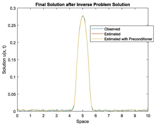
Figure 3. Simulation and estimation at time instant $t=1$ s with the noise level defined by $\eta =0.005$.

It is worth noting that the estimated data with and without the preconditioner are almost the same (at least visually). This is due to the low-level conditions used for simulation.

In order to obtain a quantitative analysis of the estimation, the relative residual is computed for this time instant. Figure 4 shows the relative residual with and without preconditioner at time instant $t=1$ s.

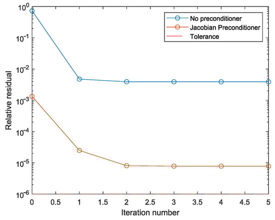
Figure 4. Relative residual with noise 0.005 at the time instant.

It can be seen from Figure 4 that the relative residual of the estimated solution with the preconditioner is lower in comparison with the estimation results without the preconditioner. This behaviour is due to the fact that preconditioning modifies the spectral properties of the system, reducing the condition number and speeding up the convergence of the iterative solver.

The proposed approach is also evaluated under higher noise-level conditions by considering a $\eta =0.05$. The same aforementioned experiments are performed for the higher noise given by $\eta =0.05$. Figure 1 shows the simulation data with noise due to $\eta =0.05$.

Figure 5, we can more clearly see the influence of the $\eta$ value.

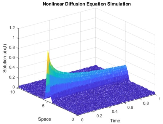
Figure 5. Simulation with a noise given by $\eta =0.05$.

Figure 6 shows the estimation data with the preconditioner.

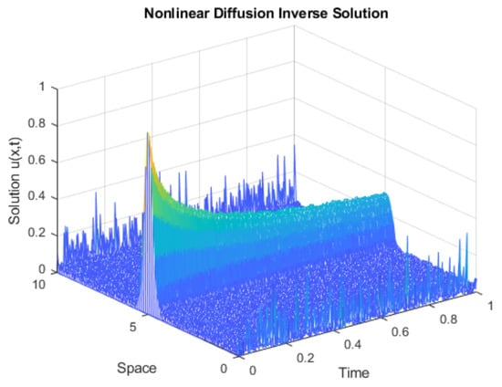
Figure 6. Estimation with a noise of $\eta =0.05$.

It can be seen that the estimated data have the same dynamics as the simulated data, but with a higher error due to the noise.

Figure 7 shows the estimation results with and without preconditioner at time instant $t=1$ s.

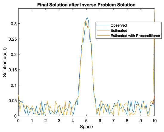
Figure 7. Simulation and estimation at time instant with noise $\eta =0.05$.

It can be seen that, in general, the estimated data with and without preconditioner approximate the simulated data under noise conditions. In order to evaluate the results by using a quantitative approach, the relative residual is computed.

Figure 8 shows the relative residual with and without preconditioner at time instant $t=1$ s.

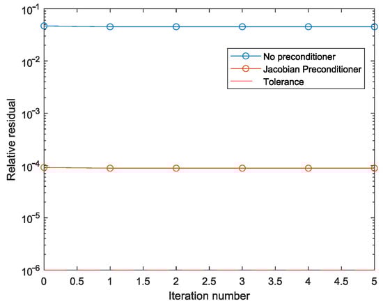
Figure 8. Relative residual with noise $\eta =0.05$ at time instant $t=1$ s.

It can be seen in Figure 8 that the initial value of the relative residual obtained by the GMRES method with the preconditioner is lower than the relative residual without the preconditioner.

4. Conclusions

This framework provides a structured approach to solving dynamic inverse problems with nonlinear diffusion models and spatiotemporal constraints. The discrete-time formulation allows efficient numerical solutions to be created using Krylov subspace methods with preconditioning, making it applicable to various scientific and engineering problems even when the dynamics are nonlinear. The proposed preconditioner based on the Jacobian approximation of the nonlinear system is also effective, speeding up the convergence of the GMRES estimation method. In addition, the proposed approach is validated in noisy conditions where the effectiveness of the preconditioner is maintained.

References

- El Madkouri, A.; Ellabib, A. A preconditioned Krylov subspace iterative method for inverse source problem by virtue of a regularizing LM-DRBEM. Int. J. Appl. Comput. Math 2020, 6, 94. [Google Scholar] [CrossRef]
- Kopaničáková, A.; Karniadakis, G.E. DeepONet based preconditioning strategies for solving parametric linear systems of equations. arXiv 2024, arXiv:2401.02016. [Google Scholar] [CrossRef]
- Pang, H.-K.; Qin, H.-H.; Ni, S. Sine transform based preconditioning for an inverse source problem of time-space fractional diffusion equations. J. Sci. Comput. 2024, 100, 74. [Google Scholar] [CrossRef]
- Gazzola, S.; Hansen, P.C.; Nagy, J.G. IR Tools: A MATLAB package of iterative regularization methods and large-scale test problems. Numer. Algorithms 2019, 81, 773–811. [Google Scholar] [CrossRef]
- Min, T.; Geng, B.; Ren, J. Inverse estimation of the initial condition for the heat equation. Int. J. Pure Appl. Math. 2013, 82, 581–593. [Google Scholar] [CrossRef]
- Kay, D.; Loghin, D.; Wathen, A. A Preconditioner for the Steady-State Navier–Stokes Equations. SIAM J. Sci. Comput. 2002, 24, 237–256. [Google Scholar] [CrossRef]
- Hansen, E.R. Preconditioning linearized equations. Computing 1997, 58, 187–196. [Google Scholar] [CrossRef]
Disclaimer/Publisher’s Note: The statements, opinions and data contained in all publications are solely those of the individual author(s) and contributor(s) and not of MDPI and/or the editor(s). MDPI and/or the editor(s) disclaim responsibility for any injury to people or property resulting from any ideas, methods, instructions or products referred to in the content. |
© 2025 by the authors. Licensee MDPI, Basel, Switzerland. This article is an open access article distributed under the terms and conditions of the Creative Commons Attribution (CC BY) license (https://creativecommons.org/licenses/by/4.0/).