Proceeding Paper

Health Monitoring of Civil Structures: A MCMC Approach Based on a Multi-Fidelity Deep Neural Network Surrogate †

1
Dipartimento di Ingegneria Civile e Ambientale, Politecnico di Milano, Piazza L. da Vinci 32, 20133 Milano, Italy
2
MOX, Dipartimento di Matematica, Politecnico di Milano, Piazza L. da Vinci 32, 20133 Milano, Italy
*
Author to whom correspondence should be addressed.
Presented at the 1st International Electronic Conference on Algorithms, 27 September–10 October 2021; Available online: https://ioca2021.sciforum.net/.
Comput. Sci. Math. Forum 2022, 2(1), 16; https://doi.org/10.3390/IOCA2021-10889
Published: 22 September 2021
(This article belongs to the Proceedings of The 1st International Electronic Conference on Algorithms)

Abstract

:
To meet the need for reliable real-time monitoring of civil structures, safety control and optimization of maintenance operations, this paper presents a computational method for the stochastic estimation of the degradation of the load bearing structural properties. Exploiting a Bayesian framework, the procedure sequentially updates the posterior probability of the damage parameters used to describe the aforementioned degradation, conditioned on noisy sensors observations, by means of Markov chain Monte Carlo (MCMC) sampling algorithms. To enable the analysis to run in real-time or quasi real-time, the numerical model of the structure is replaced with a data-driven surrogate used to evaluate the (conditional) likelihood function. The proposed surrogate model relies on a multi-fidelity (MF) deep neural network (DNN), mapping the damage and operational parameters onto sensor recordings. The MF-DNN is shown to effectively leverage information between multiple datasets, by learning the correlations across models with different fidelities without any prior assumption, ultimately alleviating the computational burden of the supervised training stage. The low fidelity (LF) responses are approximated by relying on proper orthogonal decomposition for the sake of dimensionality reduction, and a fully connected DNN. The high fidelity signals, that feed the MCMC within the outer-loop optimization, are instead generated by enriching the LF approximations through a deep long short-term memory network. Results relevant to a specific case study demonstrate the capability of the proposed procedure to estimate the distribution of damage parameters, and prove the effectiveness of the MF scheme in outperforming a single-fidelity based method.

1. Introduction

Civil structures and infrastructures are critical for the life of the world population and play a strategic role for the global economy [1]. Aging and ever-increasing extreme loading conditions threaten existing and new structural systems, stressing the need of real-time structural health monitoring (SHM) procedures to detect and identify any deviation from the damage-free baseline [2].
Vibration-based SHM techniques investigate the structural health by recording and analyzing the vibration response, e.g., acceleration or displacement multivariate time series, of the monitored structure. Two competitive SHM approaches can be formally distinguished [3]: the model-based one, e.g., [4,5], and the data-based one, e.g., [6,7]. The former is usually implemented through an updating strategy of a physics-based model on the basis of measured experimental data, which attempts to estimate the location and the extent of the occurred structural changes. The latter is based on a machine learning (ML) paradigm that, once trained, can be used as a black-box tool. ML systems automatically learn how the features, originated from the recorded data, are statistically correlated with the sought damage patterns [8]. After the advent of deep learning (DL), which can incorporate the selection and extraction of optimized features into the end-to-end learning processes, the feature engineering stage has been progressively automatized.
This work proposes an output-only approach to the damage localization problem (see for instance [9,10]), leveraging a synergic combination of multi-fidelity (MF) data-driven meta-modeling and Bayesian parameter identification. The probability distribution of the unknown damage parameters is approximated through a Markov chain Monte Carlo (MCMC) sampling algorithm.
MCMC has been applied in Bayesian model updating and model class selection in structural mechanics as well as in SHM, see, e.g., [11,12]. In this work, MCMC is used to construct a Markov chain of the sought damage parameters, whose limit distribution is the target probability distribution. The probability distribution is sequentially updated by exploring the support of the damage parameters with a density of steps proportional to the unknown posterior distribution. The sampling acceptance is governed by the evidence of the current parameters to represent sparse dynamic response measurements, as provided by a sensors network, by means of a data-driven surrogate model.
Because handling finite element (FE) simulations within an MCMC analysis is computationally impractical, a FE model capable of simulating the effect of damage on the structural response is adopted only to build labelled datasets of vibration recordings for known damage positions, see for instance [13]. A data-driven surrogate model is adopted instead to map operational and damage parameters to the associated vibration signals in place of the FE model. Such surrogate is based on a multi-fidelity deep neural network (MF-DNN) trained on synthetic data of multiple fidelities, a ML paradigm adopted and extended for instance in [14,15]. Specifically, a limited amount of high fidelity (HF) data and a lot of cheaper low fidelity (LF) data are considered. This type of meta-modeling is useful to alleviate the high demand during training of HF data, potentially expensive to collect. Indeed, the LF data supply useful information on the trends of HF data, allowing the MF-DNN to enhance the prediction accuracy only leveraging few HF data in comparison to the single-fidelity method [16].

2. SHM Methodology

The proposed methodology is detailed as follows. The composition of the datasets used to train the surrogate model is specified in Section 2.1, the considered numerical models are discussed in Section 2.2, the MF-DNN surrogate model is described in Section 2.3, and the setup of the MCMC analysis for damage localization is explained in Section 2.4.

2.1. Datasets Definition

The LF and HF datasets, respectively D LF and D HF , are built from the assembly of I LF and I HF instances, as follows
D LF = { ( x i LF , U i LF ) } i = 1 I LF , D HF = { ( x j HF , U j HF ) } j = 1 I HF ;
each LF instance is provided by a LF model of the structure to be monitored in undamaged conditions, and consists of the input parameters x i LF R N par LF defining the operational conditions, i.e., the loadings acting on the structure during the i-th instance, and the relative LF vibration time-histories U i LF ( x i LF ) = [ u 1 LF , , u N u LF ] i R N u × L shaped as N u arrays of length L. The HF counterpart is provided by a HF model of the same structure, which also accounts for the presence of structural damage and internal damping. Each HF instance consists of the input parameters x j HF R N par HF , defining the operational and damage conditions, with  N par HF > N par LF , and the associated HF vibration recordings U j HF ( x j HF ) R N u × L . As often done in the SHM literature, see for instance [3,6,12], the structural damage is modeled as a selective reduction of the material stiffness, applied to a subdomain identified by the spatial coordinates of its center θ j x j HF . For simplicity, the same sampling frequency and monitored degrees of freedom (dofs) are considered for the two fidelities, but there are no restrictions on this respect. Each instance refers to a time window ( 0 , T ) , short enough to assume steady operational, environmental, and damage conditions. In the reminder of the paper the indexes i , j will be dropped.

2.2. Datasets Population

The monitored structure is modeled as an elastic continuum discretized in space by means of a FE triangulation. The HF numerical model results from the semi-discretized form of the elasto-dynamic problem defined over the FE mesh. On the other hand, in order to ease the construction of a large LF dataset, a projection-based model order reduction strategy for parametrized systems is adopted to build the LF model, see, e.g., [9]. To this aim, the reduced basis method [17] relying on the proper orthogonal decomposition (POD)-Galerkin approach is considered. Hence, the LF approximation is obtained as a linear combination of POD-basis functions, yet not accounting for the presence of damage and structural damping. The LF and HF models read respectively as
M R d ¨ R ( t ) + K R d R ( t ) = f R ( x LF ) , t ( 0 , T ) d R ( 0 ) = W d 0 d ˙ R ( 0 ) = W d ˙ 0 ,
M d ¨ ( t ) + C ( x HF ( θ ) ) d ˙ ( t ) + K ( x HF ( θ ) ) d ( t ) = f ( x HF ) , t ( 0 , T ) d ( 0 ) = d 0 d ˙ ( 0 ) = d ˙ 0 ,
where the superscripts L and H are omitted from all the arrays for simplicity, while the superscript R stands for reduced. Having denoted by: t ( 0 , T ) the time coordinate; d ( t ) R M , d ˙ ( t ) R M and d ¨ ( t ) R M the vectors of nodal displacements, velocities and accelerations, respectively, whereas M is the number of dofs; M R M × M the mass matrix; C ( x HF ( θ ) ) R M × M the damping matrix, modeled as Rayleigh damping for mathematical convenience; K ( x HF ( θ ) ) R M × M the stiffness matrix; f ( x LF ) , f ( x HF ) R M the vectors of nodal forces; d 0 and d ˙ 0 the initial conditions at t = 0 ; W = [ w 1 , , w M R ] R M × M R the matrix gathering the M R M retained POD-basis functions; M R , K R , f R ( x LF ) , d R ( t ) the reduced arrays, playing the same role of the FE matrices but with dimension ruled by M R instead of M. It has to be noted that, even if in this case the two fidelities differ through the presence of structural damage and viscous damping in the HF model, the proposed computational framework is general and can be arbitrarily adapted to different modeling choices.
The datasets D LF and D HF are populated accordingly to Equation (1) by sampling the parametric input spaces, respectively defined by a uniform probability distribution over x LF and x HF , via latin hypercube sampling. The relevant vibration recordings U LF and U HF are extracted from d LF and d HF , respectively, through a Boolean operation.

2.3. MF-DNN Surrogate Model

The MF-DNN NN MF is composed of a LF neural network NN LF , trained on low-cost data, which is used as baseline model, and a HF neural network NN HF , trained on few HF data, which is used to adaptively learn the correlation between LF and HF data. The overall evaluation of NN MF reads as
U ^ HF = NN MF ( x HF , x LF ) = NN HF ( x HF , U ^ LF ) , U ^ LF = reshape [ Y ( 1 ω NN LF ( x LF ) ) ] ;
here: Y = [ y 1 , , y M LF ] R L concat × M LF , with  L concat = L × N u , is a matrix gathering M LF POD-basis functions built upon D L and used to compress the LF data in order to ease the complexity of NN LF ; NN LF is a fully connected DNN, mapping the LF input parameters onto the POD-basis coefficients; ω R M LF is a vector of numbers linearly decreasing from 1 to 0.2 , used to weight the regression over the POD-basis coefficients by their relative importance; ⊙ denotes the Hadamard product; the reshape operation is used to recast the reconstructed LF signals from a single vector of size L concat into N u arrays of length L; NN HF is a long short-term memory (LSTM) NN that, as more appropriate to solve time-dependent problems, is adopted to map the HF input parameters and the approximated LF signals onto the HF signals.

2.4. Damage Localization via MCMC

Accordingly to the Bayes’ rule, the posterior probability density function (pdf) of the damage parameters θ , conditioned on the observed signals U 1 , , N obs EXP is
p ( θ | U 1 , , N obs EXP , NN MF ) = p ( U 1 , , N obs EXP | θ , NN MF ) p ( θ , NN MF ) p ( U 1 , , N obs EXP | θ , NN MF ) p ( θ , NN MF ) d θ ,
where: p ( θ , NN MF ) is the prior of θ ; p ( U EXP | θ , NN MF ) is the likelihood of the evidence, which measures the goodness of fit of NN MF to U EXP given the parameters θ . By assuming that the uncertainties follow a Gaussian distribution, the likelihood function can be assumed Gaussian too thanks to the central limit theorem:
p ( U 1 , , N obs EXP | θ , NN MF ) = k N obs 1 ( 2 π ) N u | Σ c | exp 1 L τ = 1 L [ ( e τ Δ k ) Σ c 1 ( e τ Δ k ) ] 2 ;
here: N obs is the batch size of the processed observations; Δ k = U k EXP U ^ HF ( x HF ( θ ) , x LF ) is the prediction error for the k-th observation, assumed independent between different time instants and modeled as a Gaussian random vector with zero mean and covariance matrix Σ c R N u × N u , describing the spatial correlation of prediction errors due to modeling errors and measurement noise; e τ is a Boolean vector with a single non-zero entry in τ -th position, used to extract the relevant time step. For further details see, e.g., [18].
To avoid the expensive computation of the integral at the denominator of Equation (5), an MCMC sampling algorithm is adopted to approximate the posterior pdf. Specifically, the posterior pdf is sequentially updated accordingly to the Metropolis-Hastings (MH) algorithm [19]. The MH algorithm simulates a chain of θ samples distributed according to the posterior, with each sample only depending on the previous one. This generate a random walk in the space of θ , where each point is sampled with a frequency proportional to its probability. Hence, the stationary distribution of the Markov chain, under the assumption of ergodicity, asymptotically approaches the target pdf.
Let q ( ξ | θ ) be the assumed proposal pdf and δ ( θ ) = p ( U 1 , , N obs EXP | θ , NN MF ) p ( θ , NN MF ) for the sake of simplicity. The MH algorithm recursively simulate the next Markov chain sample θ k + 1 from the current sample θ k , with  k = 1 , , L chain , as follows [20]: sample a candidate ξ from q ( ξ | θ k ) ; compute the ratio α = δ ( ξ ) q ( θ k | ξ ) δ ( θ k ) q ( ξ | θ k ) ; accept the candidate ξ with probability min { 1 , α } and store it as next state of the chain, i.e.,  θ k + 1 = ξ , otherwise reject it and keep the current state of the chain, i.e.,  θ k + 1 = θ k .
After L chain states are evaluated, the burn-in period of the chain, i.e., the initial transitory phase, is removed to eliminate the initialization effect. The resulting chain is thinned up to L ˜ chain = L chain k T , with  k T a small fixed integer, in order to remove dependencies among consecutive samples. The target distribution can be ultimately approximated via histograms and the posterior expected values and covariance can be eventually approximated with the empirical mean and covariance of the θ 1 , , θ L ˜ chain samples:
μ θ = E ( θ | U 1 , , N obs EXP , NN MF ) 1 L ˜ chain l = 1 L ˜ chain θ l ,
c o v ( θ | U 1 , , N obs EXP , NN MF ) 1 L ˜ chain 1 l = 1 L ˜ chain [ θ l μ θ ] [ θ l μ θ ] .

3. Virtual Experiment

The proposed method is validated on the digital twin shown in Figure 1. The HF model in Equation () is obtained from a FE discretization resulting in M = 4659 dofs and integrated in time using the Newmark method. The structure is made of concrete, whose mechanical properties are: Young’s modulus E = 30 G P a ; Poisson’s ratio ν = 0.2 ; density ρ = 2500 k g / m 3 . The structure is excited at the tip by a distributed load q ( t ) , acting on an area of ( 0.3 × 0.3 ) m 2 , as depicted in Figure 1. The load q ( t ) varies in time according to q ( t ) = Q sin ( 2 π f t ) , where Q [ 1 , 5 ] k P a and f [ 10 , 60 ] H z respectively denote the load amplitude and frequency, collected as x LF = ( Q , f ) . Damage is introduced by reducing the material stiffness by 25 % within the subdomain Ω , which is a box ( 0.3 × 0.3 × 0.4 ) m 3 as depicted in Figure 1. The target position of this reduction is given by the coordinates of its center and can be identified with a single abscissa θ Ω [ 0.15 , 7.55 ] m running along the axis of the structure. Hence, the input parameters of the HF part are collected as x HF = ( Q , f , θ Ω ) . Also the Rayleigh damping matrix, which account for a 5 % damping ratio on the first 4 structural modes, is affected by the damage through the stiffness matrix. Synthetic displacement recordings u n ( t ) , with n = 1 , , N u , are collected from N u = 8 dofs, mimicking a monitoring system arranged as depicted in Figure 1, for a time interval ( 0 , T = 1 s ) , providing L = 200 data points.
The reduced-order model in Equation (2), i.e., the LF model used to construct D LF , has been built performing a POD upon 40,000 snapshots in time, collected while exploring the parametric input space x LF . 14 POD-bases are selected and stored in matrix W , in place of the original 4659 dofs, after having fixed a suitable tolerance on the energy norm of the reconstruction error ( tol POD = 10 3 ); for further details see, e.g., [9,13].
For the training of the surrogate model in Equation (4), I LF = 10,000 and I HF = 1000 instances have been collected from the LF and HF model, respectively. Concerning the compression of the LF data for the sake of prior dimensionality reduction, 104 POD-bases have been selected ( tol POD = 10 3 ) and stored in matrix Y , in place of 1600 data points.
The mean squared error and the mean absolute error have been used as loss functions for the training of NN LF and NN HF , respectively, together with the Adam optimization algorithm [21]. The implementation has been carried out through the Tensorflow-based Keras API [22], running on an Nvidia GeForce RTX 3080 GPU card.
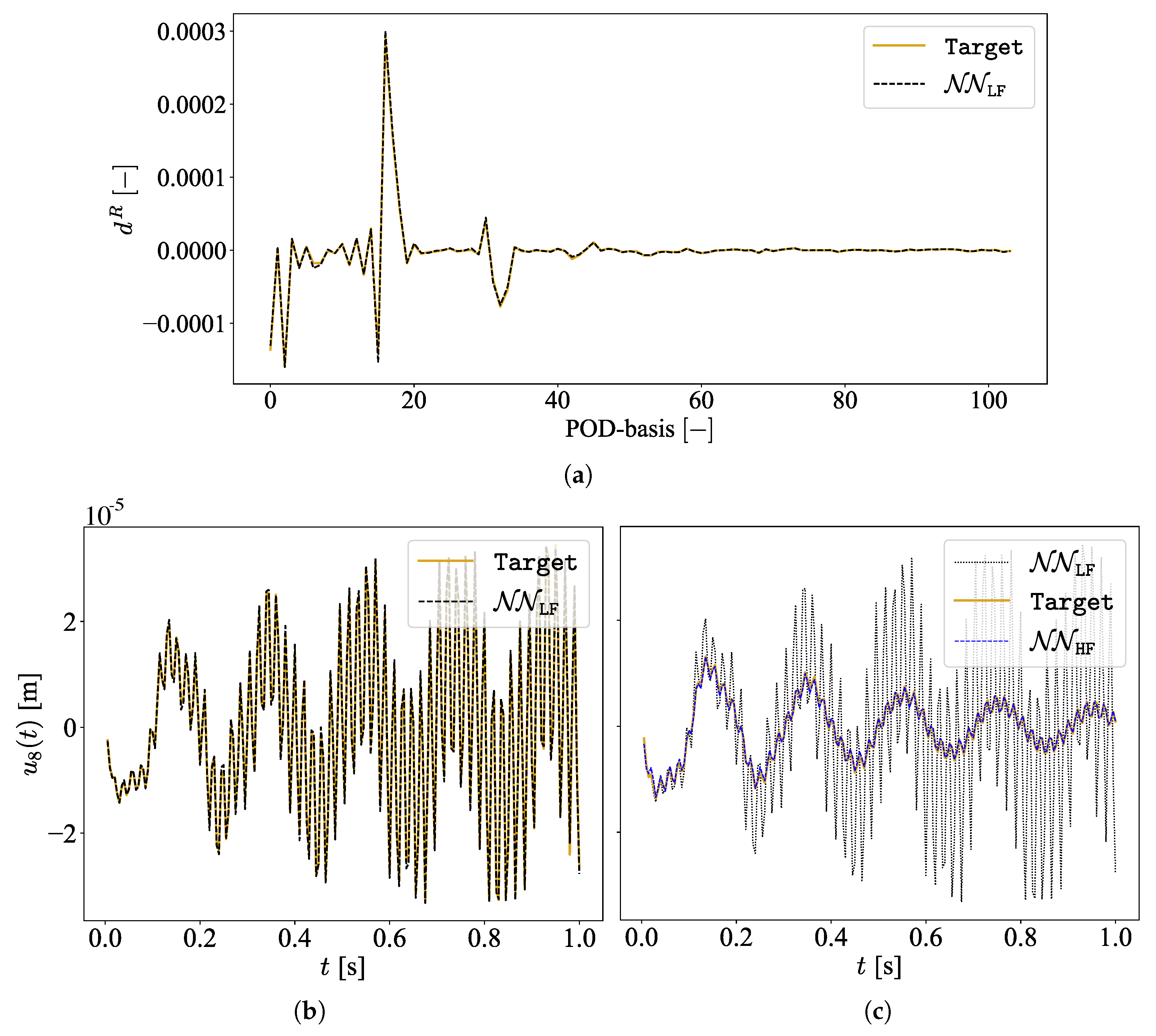
An example of the reconstruction capabilities achieved by the surrogate model is shown in Figure 2 for the monitored gdl u 8 ( t ) , where the outcome of the regression over the POD-basis coefficients, ruled by the NN LF , and the corresponding expanded LF signal are reported together with the signal enrichment, provided by the NN HF . To quantify the accuracy of the predicted signals, the Pearson correlation coefficients (PCC) between predicted and ground truth HF signals are adopted as a measure of fitness. The PCC coefficients are evaluated with respect to 40 testing instances generated with the HF model while exploring the parametric input space x HF . The minimum PCC value over the 40 testing instances for each monitored channel is respectively { 0.983 ; 0.988 ; 0.994 ; 0.995 ; 0.998 ; 0.998 ; 0.998 ; 0.998 } , which largely validate the performance of the surrogate model. The other way around, if the NN HF is employed without being coupled with the NN LF , the maximum PCC value drops to { 0.605 ; 0.603 ; 0.601 ; 0.601 ; 0.791 ; 0.735 ; 0.709 ; 0.696 } , showing the utility of the MF setting that outperforms the single-fidelity based method.
In the absence of experimental data, the Bayesian estimation of the damage parameter θ Ω is simulated by considering pseudo-experimental instances, generated with the HF model, that have been corrupted by adding independent, identically distributed Gaussian noise featuring a signal-to-noise ratio equal to 80 to each vibration recording. Batches of N obs = 3 observations relative to the same damage condition but different operational conditions are processed during the evaluation of the likelihood in Equation (6). The prior pdf p ( θ Ω , NN MF ) is taken as uniform, while, to account for the bounded domain in which θ Ω can fall, a truncated Gaussian centered on the last accepted state is considered for the proposal q ( ξ | θ Ω ) . The adaptive Metropolis [23] algorithm is adopted in order to ease the calibration of the proposal distribution, enabling its covariance to be tuned on the basis of past samples as the sampling evolves. The MCMC algorithm is run for 5000 samples, the first 500 of which are removed to get rid of the burn-in period. The obtained chain is ultimately thinned by discarding 3 samples over 4 to remove dependencies among consecutive samples.
Two examples of MCMC analyses are reported in Figure 3, showing the generated Markov chains alongside the estimated posterior mean and credibility intervals. In both cases, the damage parameter θ Ω , here normalized between 0 and 1, is properly identified. It has to be noted that the larger uncertainty in the second case is somehow expected; indeed, given the structural layout and the placing of the sensors, the sensitivity of measures to damage positions far apart from the clamped side is smaller.

4. Conclusions

This paper has presented a stochastic approach for SHM, here applied to the problem of damage localization in case of slow damage progression. The presence of damage has been postulated as already detected, e.g., as identified by an early warning tool, and only the localization task has been analyzed. The Bayesian identification of damage parameters is achieved through an MCMC sampling algorithm, adopted to approximate their posterior distribution conditioned on a set of measurements. Few investigations are present in literature involving the use of MCMC for the health monitoring of civil structures, and this is the first one considering a MF-DNN surrogate model to accelerate the computation of the conditional likelihood. The surrogate model learns from simulated data of multiple fidelities, i.e., few HF data and several inexpensive LF data, such to alleviate the computational burden of the supervised training stage. The method has been assessed on a numerical case study, showing remarkable accuracy under the effect of measurement noise and varying operational conditions.
The method is suitable for structural typologies whose damage patterns can be represented by a stiffness reduction fixed within the time interval of interest. Since it enables a time scale separation between damage growth and damage assessment, this is a standard assumption for most practical scenarios in SHM. Such description of damage is consistent with the adopted vibration-based SHM approach, and allows the structure to be modeled as a linear system both in the presence and absence of damage. Moreover, as shown in [9], even if the stiffness reduction takes place over domains of different size from that one adopted during the dataset construction, it is still possible to identify the correct position of damage.
Considering data-driven algorithms, damage localization is often addressed by exploiting a DL feature extractor followed by a classification or a regression module, e.g., as done in [9,10,13]. However, due to the need of training in a simulated environment, the risk of losing generalization capabilities on real monitoring data is high. The proposed procedure tries to overcomes such generalization problems. Damage is located by seeking for those parameters of the surrogate model producing the closest output to the measured one, in terms of a suitable distance function measuring the signals similarity. For this reason and thanks to the fully stochastic framework here considered, which is suitable for dealing with noisy data and modeling inaccuracies, it is reasonable to expect a better ability of generalizing outside the training regime.
Besides the need of validating the proposed methodology within a suitable experimental setting, the next studies will extended the Bayesian identification also to the parameters controlling the operational conditions. Moreover, a usage monitoring tool powered by a suitable data-driven paradigm will be considered to provide useful prior knowledge as opposite to an informative flat prior. The analysis of dynamic effects resulting from localized damage mechanisms is also left for future investigations.

Author Contributions

Conceptualization, M.T., A.M. and S.M.; methodology, M.T., A.M. and S.M.; software, M.T.; validation, M.T., A.M. and S.M.; formal analysis, M.T., A.M. and S.M.; investigation, M.T.; resources, A.M. and S.M.; data curation, M.T.; writing—original draft preparation, M.T.; writing—review and editing, M.T., A.M. and S.M.; visualization, M.T.; supervision, A.M. and S.M.; project administration, A.M. and S.M.; funding acquisition, A.M. and S.M. All authors have read and agreed to the published version of the manuscript.

Funding

This research received no external funding.

Institutional Review Board Statement

Not applicable.

Informed Consent Statement

Not applicable.

Data Availability Statement

All data generated during the study are available from the corresponding author upon reasonable request.

Acknowledgments

M.T. acknowledges the financial support by Politecnico di Milano through the interdisciplinary Ph.D. Grant “Physics-Informed Deep Learning for Structural Health Monitoring”.

Conflicts of Interest

The authors declare no conflict of interest.

References

  1. Flah, M.; Nunez, I.; Ben Chaabene, W.; Nehdi, M.L. Machine Learning Algorithms in Civil Structural Health Monitoring: A Systematic Review. Arch. Comput. Methods Eng. 2021, 28, 2621–2643. [Google Scholar] [CrossRef]
  2. Mariani, S.; Azam, S.E. Health Monitoring of Flexible Structures Via Surface-mounted Microsensors: Network Optimization and Damage Detection. In Proceedings of the 5th ICRAE, Singapore, 20–22 November 2020; pp. 81–86. [Google Scholar] [CrossRef]
  3. Worden, K. Structural fault detection using a novelty measure. J. Sound Vib. 1997, 201, 85–101. [Google Scholar] [CrossRef]
  4. Corigliano, A.; Mariani, S. Parameter identification in explicit structural dynamics: Performance of the extended Kalman filter. Comput. Methods Appl. Mech. Eng. 2004, 193, 3807–3835. [Google Scholar] [CrossRef]
  5. Eftekhar Azam, S.; Chatzi, E.; Papadimitriou, C. A dual Kalman filter approach for state estimation via output-only acceleration measurements. Mech. Syst. Signal Process. 2015, 60–61, 866–886. [Google Scholar] [CrossRef]
  6. Farrar, C.; Worden, K. Structural Health Monitoring A Machine Learning Perspective; John Wiley & Sons: Hoboken, NJ, USA, 2013. [Google Scholar]
  7. Fink, O.; Wang, Q.; Svensen, M.; Dersin, P.; Lee, W.; Ducoffe, M. Potential, Challenges and Future Directions for Deep Learning in Prognostics and Health Management Applications. Eng. Appl. Artif. Intell. 2020, 92, 103678. [Google Scholar] [CrossRef]
  8. Bishop, C.M. Pattern Recognition and Machine Learning (Information Science and Statistics); Springer: Berlin/Heidelberg, Germany, 2006. [Google Scholar]
  9. Rosafalco, L.; Torzoni, M.; Manzoni, A.; Mariani, S.; Corigliano, A. Online structural health monitoring by model order reduction and deep learning algorithms. Comput. Struct. 2021, 255, 106604. [Google Scholar] [CrossRef]
  10. Sajedi, S.O.; Liang, X. Vibration-based semantic damage segmentation for large-scale structural health monitoring. Comput.-Aided Civ. 2020, 35, 579–596. [Google Scholar] [CrossRef]
  11. Mirzazadeh, R.; Eftekhar Azam, S.; Mariani, S. Mechanical characterization of polysilicon MEMS: A hybrid TMCMC/POD-kriging approach. Sensors 2018, 18, 1243. [Google Scholar] [CrossRef] [PubMed] [Green Version]
  12. Lam, H.F.; Yang, J.H.; Au, S.K. Markov chain Monte Carlo-based Bayesian method for structural model updating and damage detection. Struct. Contr. Health Monit. 2018, 25, e2140. [Google Scholar] [CrossRef]
  13. Torzoni, M.; Rosafalco, L.; Manzoni, A. A Combined Model-Order Reduction and Deep Learning Approach for Structural Health Monitoring Under Varying Operational and Environmental Conditions. Eng. Proc. 2020, 2, 94. [Google Scholar] [CrossRef]
  14. Meng, X.; Babaee, H.; Karniadakis, G.E. Multi-fidelity Bayesian Neural Networks: Algorithms and Applications. J. Comput. Phys. 2021, 438, 110361. [Google Scholar] [CrossRef]
  15. Guo, M.; Manzoni, A.; Amendt, M.; Conti, P.; Hesthaven, J.S. Multi-fidelity regression using artificial neural networks: Efficient approximation of parameter-dependent output quantities. arXiv 2021, arXiv:2102.13403. [Google Scholar] [CrossRef]
  16. Meng, X.; Karniadakis, G.E. A composite neural network that learns from multi-fidelity data: Application to function approximation and inverse PDE problems. J. Comput. Phys. 2020, 401, 109020. [Google Scholar] [CrossRef] [Green Version]
  17. Quarteroni, A.; Manzoni, A.; Negri, F. Reduced Basis Methods for Partial Differential Equations: An Introduction; Springer: Berlin/Heidelberg, Germany, 2015. [Google Scholar]
  18. Papadimitriou, C.; Lombaert, G. The effect of prediction error correlation on optimal sensor placement in structural dynamics. Mech. Syst. Signal Process. 2012, 28, 105–127. [Google Scholar] [CrossRef]
  19. Hastings, W.K. Monte Carlo Sampling Methods Using Markov Chains and Their Applications. Biometrika 1970, 57, 97–109. [Google Scholar] [CrossRef]
  20. Goulet, J.A. Probabilistic Machine Learning for Civil Engineers; MIT Press: Cambridge, MA, USA, 2020. [Google Scholar]
  21. Kingma, D.; Ba, J. Adam: A Method for Stochastic Optimization. In Proceedings of the 3rd ICLR, San Diego, CA, USA, 7–9 May 2015; pp. 1–13. [Google Scholar]
  22. Keras. 2015. Available online: https://keras.io (accessed on 24 February 2022).
  23. Haario, H.; Saksman, E.; Tamminen, J. An adaptive Metropolis algorithm. Bernoulli 2001, 7, 223–242. [Google Scholar] [CrossRef] [Green Version]
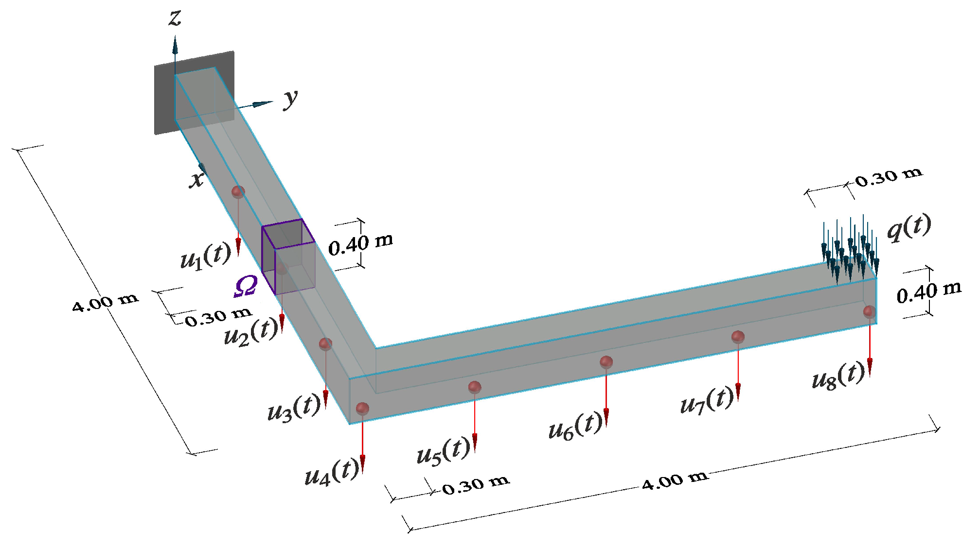
Figure 1. Physics-based digital twin of the monitored structure.
Csmf 02 00016 g001
Figure 2. Reconstruction capacity of NN MF : (a) regression over the POD-basis coefficients relative to a compressed LF signal; (b) decompressed LF signal; (c) regression over the HF signal.
Csmf 02 00016 g002
Figure 3. Examples of MCMC analysis, in case of damage position (a) close to the clamped side and (b) far from the clamped side.
Csmf 02 00016 g003
Publisher’s Note: MDPI stays neutral with regard to jurisdictional claims in published maps and institutional affiliations.