Proceeding Paper

Comparing Machine Learning Methods—SVR, XGBoost, LSTM, and MLP— For Forecasting the Moroccan Stock Market †

Laboratory LMSA, Department of Mathematics, Faculty of Sciences, Mohammed V University in Rabat, Rabat 10000, Morocco
*
Author to whom correspondence should be addressed.
Presented at the 1st International Online Conference on Mathematics and Applications, 1–15 May 2023; Available online: https://iocma2023.sciforum.net/.
Comput. Sci. Math. Forum 2023, 7(1), 39; https://doi.org/10.3390/IOCMA2023-14409
Published: 28 April 2023

Abstract

:
Forecasting and modeling time series is a crucial aspect of economic research for academics and business practitioners. The ability to predict the direction of stock prices is vital for creating an investment plan or determining the optimal time to make a trade. However, market movements can be complex to predict, non-linear, and chaotic, making it difficult to forecast their evolution. In this paper, we investigate modeling and forecasting the daily prices of the new Morocco Stock Index 20 (MSI 20). To this end, we propose a comparative study between the results obtained from the application of the various Machine Learning (ML) methods: Support Vector Regression (SVR), eXtreme Gradient Boosting (XGBoost), Multilayer Perceptron (MLP), and Long Short-Term Memory (LSTM) models. The results show that using the Grid Search (GS) optimization algorithm, the SVR and MLP models outperform the other models and achieve high accuracy in forecasting daily prices.

1. Introduction

The 2008 recession, the stock market crash of 2015, the COVID-19 Pandemic, and the Russian Invasion of Ukraine are some of the most recent crises which have had an immense impact on the financial markets and the destruction of wealth worldwide. Modeling and forecasting the stock market is a challenge that many engineers and financial researchers face. The literature review examined studies on stock market prediction using Machine Learning (ML) models. It concluded that Deep Learning (DL) was the most commonly utilized model for forecasting stock price trends [1,2]. Traditional econometric methods might require improved performance in relevant nonlinear time series and may not be appropriate for directly forecasting stock prices because of their volatility [3]. However, for complex nonlinear financial time series, methods such as Support Vector Regression (SVR), eXtreme Gradient Boosting (XGBoost), Multilayer Perceptron (MLP), and Long Short-Term Memory (LSTM) can detect nonlinear relationships in the forecasting of stock prices [4] and achieve better fitting results by tuning multiple parameters [5]. Hyperparameter optimization or tuning in ML refers to selecting the most appropriate parameters for a particular learning model [6]. Some studies use Grid Search (GS) optimization [7], while others use Bayesian [8,9] or pigeon-inspired optimization algorithms [10]. In this paper, the GS algorithm is used to optimize the parameters of each model, such as SVR, XGBoost, MLP, and LSTM models. Then, we compare them using seven measures: Mean Error (ME), Mean Percentage Error (MPE), Mean Square Error (MSE), Mean Absolute Error (MAE), Root Mean Square Error (RMSE), Mean Absolute Percentage Error (MAPE), and R 2 . In [11], it was discovered that using LSTM with Moving Averages (MA) yields superior results for predicting stock prices compared to SVR, as measured by different performance criteria such as MAE, MSE, MAPE, RMSE, and R 2 values. In their research [12], Al-Nefaie et al. proposed using LSTM and MLP models to forecast the fluctuations in the Saudi stock market. They found that the correlation coefficient for the two models was higher than 0.995. The LSTM model proved to have the highest accuracy and best model fit. In [13], the authors compared performance measures such as MSE, MAE, RMSE, and MAPE to forecast stock market trends based on Auto-Regressive Integrated Moving Average (ARIMA), XGBoost, and LSTM. Their tests found that XGBoost performed the best. In a different context, ML methods such as ANN and MLP [14] were used to forecast solar irradiance. The results indicate that the MLP model with exogenous variables performs better than the other models. Similarly, in another study [15], the predictive performance and stability of eXtreme Gradient Boosting Deep Neural Networks (XGBF-DNN) made it an optimal and reliable model for forecasting hourly global horizontal irradiance using the GS algorithm. The main objective of this investigation is to improve the GS optimization algorithm by optimizing the hyperparameters of ML models. Furthermore, this study compares two ML methods and two DL methods. To achieve this objective, the research includes an in-depth literature review of 20 studies on ML models for stock market prediction. Overall, the paper aims to contribute to the stock market prediction field by improving the performance of ML models through hyperparameter optimization. Our contribution is highlighted in Table 1, which offers a more accurate prediction than other studies.
The rest of this paper is organized as follows: Section 2 outlines the suggested methodology for modeling and forecasting financial time series, specifically stock prices. Section 3 details the implementation of the study, results, and discussion. Lastly, Section 4 offers conclusions and suggests future research directions.

2. Materials and Methods

This section provides an overview of the methodology employed in this research.

2.1. Data Collection

This research focuses on modeling and forecasting a new Moroccan Stock Index 20 (MSI 20) composed of the most liquid companies listed on the Casablanca Stock Exchange (CSE) from various sectors, including Attijariwafa Bank, Itissalat Al-Maghrib, Banque Populaire, LafargeHolcim Morocco, … etc. The MSI 20 is calculated in real time during the business hours of the CSE from Monday to Friday, and from 9:00 a.m. to 3:30 p.m. local time (Limited on weekends and holidays). The research was conducted using the Python software. In addition, several libraries were used, including Matplotlib, Pandas, NumPy, Sklearn, Tensorflow, and Keras. We use daily MSI 20 data to train each model and predict closing prices. Since the launch of the index of length N = 541 , we use prices as Input = (Open, High, Low, and Closing prices), see the Table 2 below:
To train model parameters, we use historical data of length N,
X = { X t ( 1 ) , X t ( 2 ) , X t ( 3 ) , t = 1 , 2 , , N } ,
where X ( i ) with i = 1 , 2 , 3 represents the Open, High, and Low prices, respectively. For the output with a single observation sequence, we use only closing price,
Y = Y t , t = 1 , 2 , , N

2.2. Preprocessing

The dataset was divided into 90% of the observations used for training and 10% for model evaluation during testing. Data preprocessing is an essential step in ML that helps achieve competitive results and eliminate metric unit effects. In this case, we normalized using a min–max scale, which scales all variables to a range of [ 0 , 1 ] :
X ˜ t = X t X t m i n X t m a x X t m i n
where X t represents the historical data for each feature variable in the time series (Open, High, and Low prices) and the X t m a x and X t m i n values are the sample’s maximum and minimum values.

2.3. SVR Model

The SVR model, a new financial time series prediction method, is used to address the challenges of nonlinear regression. We assume a linear relationship exists between X t and Y t as in the left side of the Equation (2). To perform nonlinear regression using SVR, the concept consists of creating an x φ ( x ) transformation that maps the original feature space X, which has N dimensions, onto the new feature space X . Mathematically, this can be explained by the equation shown below:
Y t = W · X t + b = i = 1 N w i x i t + b i , m a p p i n g N o n l i n e a r Y t = k β k y k K ( x k , x ) + b
where w i is the vector of weights and b i is a bias, β k is the coefficient of the Lagrange multipliers, and K ( x k , x ) = φ ( x k ) · φ ( x ) is a kernel function. The most commonly used kernels include linear, Gaussian, and polynomial functions [17].

2.4. XGBoost Model

XGBoost is an ML model used for stock market time series forecasting that uses a set of decision trees [18]. A gradient descent algorithm guides the process of preparing subsequent trees to minimize the loss function of the last tree [6].
L T ( F ( x i ) ) = i = 1 N χ ( y i , F T ( x i ) ) + t = 1 T Π ( f t ) ,
where χ ( · ) is a specified loss function that quantifies the deviations of the predicted and actual target values, and F T ( x i ) = t = 1 T f t ( x i ) denotes the forecast on the i-th sample at the T-th boost and Π ( f ) = α K + 0.5 × κ ϖ 2 , where K is the number of leaves. For the regularization term, α is the parameter of complexity. ϖ 2 is the L2 norm of weight regularization, κ is a constant coefficient, and Π ( · ) represents the term of regularization, which penalizes the model complexity [8].

2.5. MLP Model

The MLP is a frequently used ANN consisting of three layers of neurons: an input layer, one or more hidden layers, and an output layer. The inputs ( x i ) are multiplied by their weights ( w i ), and the resulting products are combined. This sum and a bias term (b) are fed into an activation function to produce the neuron’s output ( Y t ) [19]. Equation (2) can be used to express this process in mathematical words:
ζ t = i = 1 N w i x i t + b Y t = σ ( ζ t ) ,
σ ( ζ t ) = 1 1 + e ζ t
where σ ( · ) , the activation function, is frequently employed as a function, either continuous or discontinuous, that maps real numbers to a specific interval. Alternatively, the sigmoidal activation function can also be utilized [12].

2.6. LSTM Model

LSTM models are RNNs that excel at learning and retaining long-term dependencies, making them successful in various applications such as financial time series forecasting. The principle of an LSTM cell consists of the following four equations [20]:
Forget gate: f t = δ ( W e f · ( X t , h t 1 ) + W c f C t 1 + b f ) , Input gate: i t = δ ( W k i · ( X t , h t 1 , C t 1 ) + b i ) , k = x , h , c Memory cell:    C t = f t · C t 1 + i t · tanh ( W l c ( X t , h t 1 ) + b c ) , l = x , h Output gate:     o t = δ ( W j i · ( X t , h t 1 , C t 1 ) + b o ) , j = x , h , c
where W e * , W c * , W k * , W l * , W j * , and b f , b i , b c , b o are the weight and bias of each layer respectively, and h t = o t · tanh ( C t ) represents the hidden layer output. The forget gate ( f t ) determines if the information should be kept or discarded, while the input gate ( i t ) integrates new data into the cell ( C t ). Eventually, the output gate ( o t ) governs the selection of relevant data to transmit to the succeeding cell ( C t 1 ).

2.7. Grid Search

In ML, GS is commonly used to fine-tune parameters such as regularization strength, learning rate, several hidden layers …, etc. By using the GS algorithm, we can identify the optimal set of hyperparameters for the models, resulting in better predictions and improved performance. In our case, we first defined the hyperparameters and their search space, as shown in the Table 3. The optimal hyperparameters for each model are shown below in bold blue. The design of the research study is illustrated in Figure 1.

3. Results and Discussion

In the section on results and discussion, we report and compare the performance of the SVR, XGBoost, MLP, and LSTM models for forecasting the MSI 20 stock market. Various evaluation measures such as ME, MPE, MSE, MAE, RMSE, MAPE, and R 2 scores are obtained to assess the models’ accuracy. Let y ^ i t be the forecast of model i in time t, while y t is the real value in time t, y ¯ t is the mean value, and n is the length of the set time series (i.e., training and test sets). The error for model i at time t is defined as ε i t = y t y ^ i t . The general formula for evaluation measures is presented in Table 4 below:
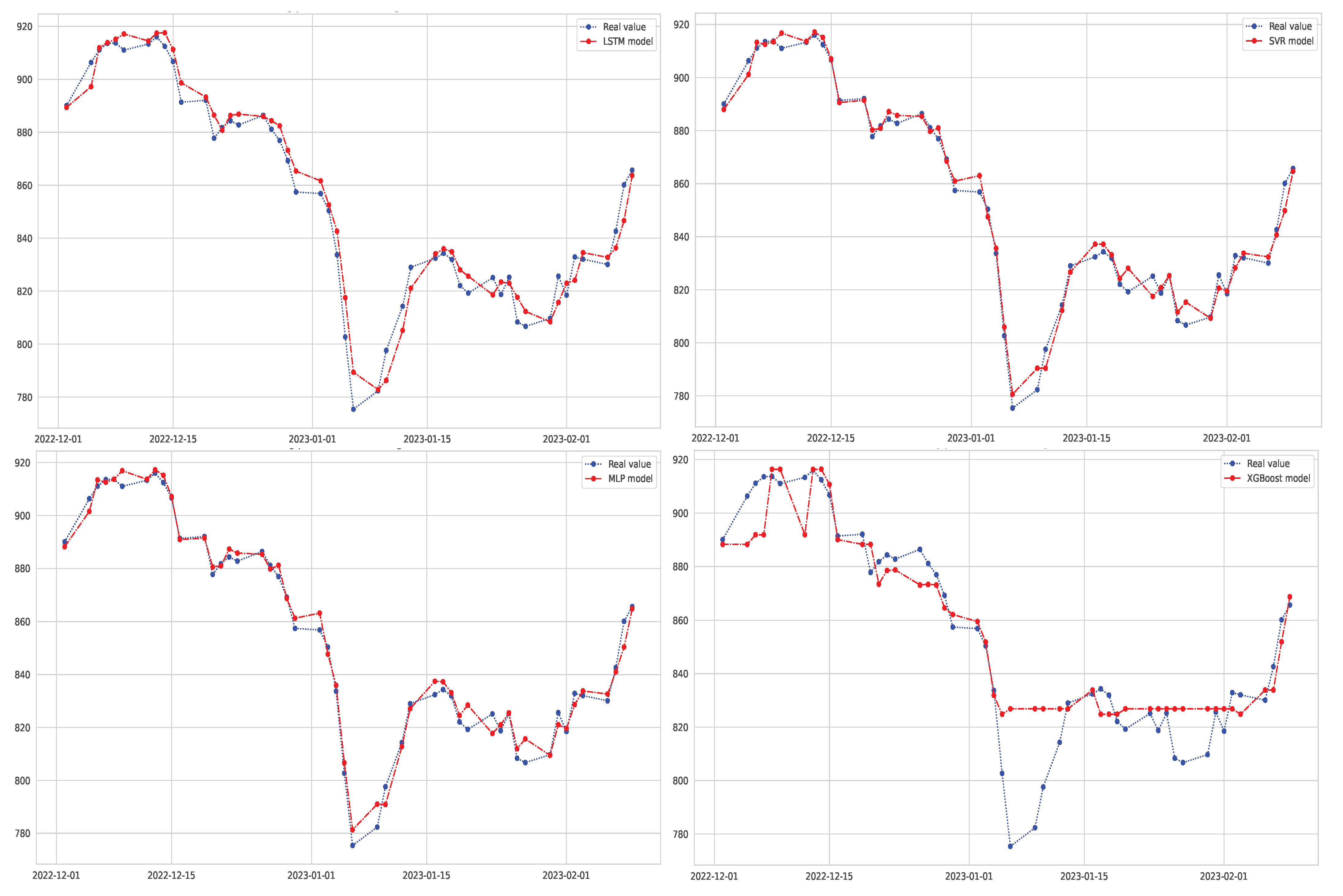
Table 5 shows the evaluation values of various forecasting models for the MSI 20 price. XGBoost had the highest error among the four models. LSTM had the second-worst performance. SVR and MLP models had lower performance metrics than XGBoost and LSTM models. However, the SVR model had the best evaluation values for forecasting MSI 20 prices, achieving optimal ME, MAE, RMSE, MPE, MAPE, and MSE values of 0.674, 3.092, 3.993, 0.082%, 0.368%, and 15.941, respectively. The MLP model also showed excellent performance metrics. However, the predicted results of the XGBoost model in Figure 2 on the right showed a specific error. They predicted values of MSI 20, especially during the fall period (6 January 2023–10 January 2023 ), indicating that the model needed more data to improve its performance. Based on the results presented in Table 5 and Figure 2, it can be concluded that the SVR model followed by MLP models had the best performance for forecasting MSI 20 compared to other models.

4. Conclusions and Future Work

This study applied four machine learning models—SVR, XGBoost, MLP, and LSTM—to model and forecast MSI 20 prices using multivariate time series data. The results showed that SVR outperformed the other models with lower errors and higher accuracy 98.9%. Future research could focus on improving the performance of XGBoost and exploring the potential of other models, such as CNN-LSTM, for stock market forecasting.

Author Contributions

H.O. and K.E.H. contributed equally to this manuscript. All authors have read and agreed to the published version of the manuscript.

Funding

This research received no external funding.

Informed Consent Statement

Not applicable.

Data Availability Statement

The data is available on the CSE website: https://www.casablanca-bourse.com (accessed on 10 February 2020).

Acknowledgments

We appreciate all the reviewers who helped us improve the paper.

Conflicts of Interest

The authors declare no conflict of interest.

References

  1. Mintarya, L.N.; Halim, J.N.; Angie, C.; Achmad, S.; Kurniawan, A. Machine learning approaches in stock market prediction: A systematic literature review. Procedia Comput. Sci. 2023, 216, 96–102. [Google Scholar] [CrossRef]
  2. Ozbayoglu, A.M.; Gudelek, M.U.; Sezer, O.B. Deep learning for financial applications: A survey. Appl. Soft Comput. 2020, 93, 106384. [Google Scholar] [CrossRef]
  3. Li, R.; Han, T.; Song, X. Stock price index forecasting using a multiscale modeling strategy based on frequency components analysis and intelligent optimization. Appl. Soft Comput. 2022, 124, 109089. [Google Scholar] [CrossRef]
  4. Kim, T.; Kim, H.Y. Forecasting stock prices with a feature fusion LSTM-CNN model using different representations of the same data. PLoS ONE 2019, 14, e0212320. [Google Scholar] [CrossRef] [PubMed]
  5. Xu, S.; Zou, S.; Huang, J.; Yang, W.; Zeng, F. Comparison of Different Approaches of Machine Learning Methods with Conventional Approaches on Container Throughput Forecasting. Appl. Sci. 2022, 12, 9730. [Google Scholar] [CrossRef]
  6. Yang, L.; Shami, A. On hyperparameter optimization of machine learning algorithms: Theory and practice. Neurocomputing 2020, 415, 295–316. [Google Scholar] [CrossRef]
  7. Rubio, L.; Alba, K. Forecasting Selected Colombian Shares Using a Hybrid ARIMA-SVR Model. Mathematics 2022, 10, 2181. [Google Scholar] [CrossRef]
  8. Xia, Y.; Liu, C.; Li, Y.; Liu, N. A boosted decision tree approach using Bayesian hyper-parameter optimization for credit scoring. Expert Syst. Appl. 2017, 78, 225–241. [Google Scholar] [CrossRef]
  9. Liwei, T.; Li, F.; Yu, S.; Yuankai, G. Forecast of LSTM-XGBoost in Stock Price Based on Bayesian Optimization. Intell. Autom. Soft Comput. 2021, 29, 855–868. [Google Scholar] [CrossRef]
  10. Al-Thanoon, N.A.; Algamal, Z.Y.; Qasim, O.S. Hyper parameters Optimization of Support Vector Regression based on a Chaotic Pigeon-Inspired Optimization Algorithm. Math. Stat. Eng. Appl. 2022, 71, 4997–5008. [Google Scholar]
  11. Lakshminarayanan, S.K.; McCrae, J.P. A Comparative Study of SVM and LSTM Deep Learning Algorithms for Stock Market Prediction. In Proceedings of the AICS, Wuhan, China, 12–13 July 2019; pp. 446–457. [Google Scholar]
  12. Al-Nefaie, A.H.; Aldhyani, T.H. Predicting Close Price in Emerging Saudi Stock Exchange: Time Series Models. Electronics 2022, 11, 3443. [Google Scholar] [CrossRef]
  13. Goverdhan, G.; Khare, S.; Manoov, R. Time Series Prediction: Comparative Study of ML Models in the Stock Market. Res. Sq. 2022. [Google Scholar] [CrossRef]
  14. Ettayyebi, H.; El Himdi, K. Artificial neural network for forecasting one day ahead of global solar irradiance. In Proceedings of the Smart Application and Data Analysis for Smart Cities (SADASC’18), Casablanca, Morocco, 27–28 February 2018. [Google Scholar]
  15. Kumari, P.; Toshniwal, D. Extreme gradient boosting and deep neural network based ensemble learning approach to forecasting hourly solar irradiance. J. Clean. Prod. 2021, 279, 123285. [Google Scholar] [CrossRef]
  16. Lu, W.; Li, J.; Li, Y.; Sun, A.; Wang, J. A CNN-LSTM-based model to forecast stock prices. Complexity 2020, 2020, 6622927. [Google Scholar] [CrossRef]
  17. Ranković, V.; Grujović, N.; Divac, D.; Milivojević, N. Development of support vector regression identification model for prediction of dam structural behavior. Struct. Saf. 2014, 48, 33–39. [Google Scholar] [CrossRef]
  18. Dezhkam, A.; Manzuri, M.T. Forecasting stock market for an efficient portfolio by combining XGBoost and Hilbert–Huang transform. Eng. Appl. Artif. Intell. 2023, 118, 105626. [Google Scholar] [CrossRef]
  19. Koukaras, P.; Nousi, C.; Tjortjis, C. Stock Market Prediction Using Microblogging Sentiment Analysis and Machine Learning. Telecom 2022, 3, 358–378. [Google Scholar] [CrossRef]
  20. Wu, J.M.T.; Li, Z.; Herencsar, N.; Vo, B.; Lin, C.W. A graph-based CNN-LSTM stock price prediction algorithm with leading indicators. Multimed. Syst. 2021, 29, 1751–1770. [Google Scholar] [CrossRef]
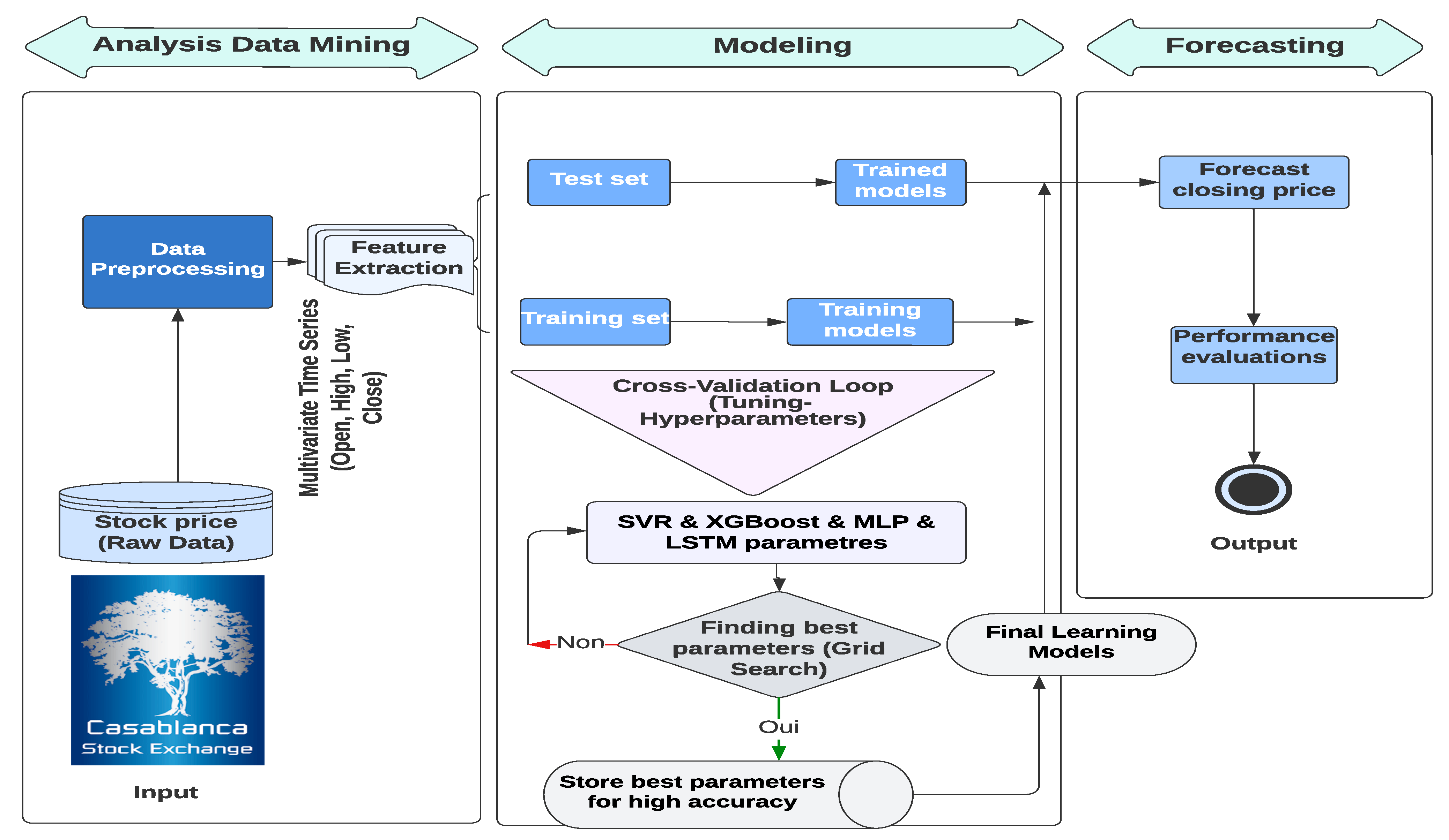
Figure 1. The proposed research design architecture for analyzing, modeling, and predicting MSI 20.
Csmf 07 00039 g001
Figure 2. MSI 20 stock price prediction: results of LSTM, SVR, MLP, and XGBoost models.
Csmf 07 00039 g002
Table 1. Some previous work using ML models for stock market forecasting.
ReferenceLocationYearBenchmark ModelMAPE (%)RMSER 2
[11]Irlande2019LSTM, SVR, MA1.03347.460.83
[16]China2020MLP, CNN, RNN, LSTM, CNN-RNN39.6880.965
[13]American2022ARIMA, XGBoost, LSTM3.86.1010.961
This studyMorocco2023SVR, XGBoost, MLP, LSTM0.3683.9930.989
The abbreviations have the following meaning: RNN = Recurrent Neural Network, CNN = Convolutional Neural Network.
Table 2. Sample data (First five days) and descriptive statistics of MSI 20 index daily prices from 18 December 2020 to 9 February 2023.
Trade DateOpen (MAD)High (MAD)Low (MAD)Close (MAD)
2020-12-18946.25950.56943.85944.58
2020-12-21944.58944.58911.51912.17
2020-12-22912.17928.51906.77927.79
2020-12-23927.79935.71927.07932.43
2020-12-24932.43932.81926.58927.16
StatisticsOpenHighLowClose
Count541541541541
Mean988.86993.28984.91988.84
Std78.0177.0578.3578.15
Min775.38797.01775.38775.38
Max1140.691142.561135.861140.69
Note: MAD = Moroccan Dirham.
Table 3. The GS hyper-parameter sets for the SVR, XGBoost, MLP, and LSTM models.
ML ModelsParametersTypeSearch Space
Epsilon in the SVR loss function (epsilon)Continuous[0.0001, 0.001, 0.01]
Regularization parameter (C)Discrete[100, 1000, 1100]
SVRThe kernel type (kernel)Categorical[’linear’, ’poly’, ’rbf’, ’sigmoid’]
Kernel coefficient (gamma)Continuous[1 × 10⁻⁵, 1 × 10⁻⁴, 1 × 10⁻³]
Tolerance for stopping criterion (tol)Continuousdefault = 1 × 10⁻³
# of regression trees (n_estimators)Discrete[100, 200, 1000]
Maximum regression tree depth (max_depth)Discrete[5,10, 15, 20]
Boosting the rate of learning (learning_rate)Continuous[0.01, 0.06, 0.09]
XGBoostMinimum reduction of loss (gamma)Continuous[0.001, 0.01, 0.1]
Regularization term L1 on weights (reg_alpha)Continuous[ 0.001, 0.01, 0.1]
Regularization term L2 on weights (reg_lambda)Continuous[ 0.001, 0.01, 0.1]
Objective learning function (objective)Categorical[’reg:squarederror’,’reg:linear’]
# of neurons in the ith hidden layer (hidden_layer_sizes)Discrete[(50,50,50), (50,100,50), (100,)]
Activation function for hidden layer (activation)Categorical[’relu’,’tanh’,’logistic’,’identity’]
MLPThe solver for weight optimization (solver)Categorical[’sgd’,’adam’,’lbfgs’]
Strength of the regularization term L2 (alpha)Continuous[0.001, 0.01, 0.1]
Learning rate for weight update program (learning_rate)Categorical[’constant’,’invscaling’,’adaptive’]
# of epochs to train the model (epochs)Discrete[20, 90, 100]
# of hidden layerDiscrete[1, 2, 3, 4]
The function that tries to optimize (optimizer)Categorical[’adam’,’rmsprop’,’sgd’]
LSTMLearning rate (learning_rate)Continuous[0.1, 0.01, 0.001]
Activation functions (activation)Categorical[’tanh’,’sigmoid’,’relu’]
# of hidden layer neurons (neurons_1, neurons_2)Discrete[150, 250, 350], [200, 200, 300],
Loss functions to be minimized during model training (loss)Categorical[’mae’,’mse’,’mape’]
Table 4. Formulas for model performance measures.
MetricsMEMAEMSEMPE (%)MAPE (%)RMSER 2 (%)
Formulas 1 n t = 1 n ε i t 1 n t = 1 n | ε i t | 1 n t = 1 n ε i t 2 100 n t = 1 n ε i t y t 100 n t = 1 n | ε i t y t | MSE 1 n MSE t = 1 n ( y t y ¯ t )
Table 5. The performance analysis measures metrics of each model.
ModelsSVRXGBoostMLPLSTM
Error MeasureTrainingTestTrainingTestTrainingTestTrainingTest
ME0.08990.6742.2770.5585.406 × 10 6 0.8832.3391.4
MAE2.0583.0922.4609.1652.0593.1013.5545.065
RMSE2.6463.9933.14113.5152.6424.0184.4966.322
MPE (%) 9.134 × 10 3 0.0820.2260.1167.603 × 10 4 0.1070.1640.234
MAPE (%)0.2070.3680.2441.0950.2070.3700.3570.603
MSE7.00315.9419.864182.6516.97816.28620.21539.97
R 2 0.9980.9890.9970.8820.9980.9890.9950.974
Disclaimer/Publisher’s Note: The statements, opinions and data contained in all publications are solely those of the individual author(s) and contributor(s) and not of MDPI and/or the editor(s). MDPI and/or the editor(s) disclaim responsibility for any injury to people or property resulting from any ideas, methods, instructions or products referred to in the content.