First-Order Decay Models for the Estimation of Methane Emissions in a Landfill in the Metropolitan Area of Oaxaca City, Mexico

Abstract

Methane is a powerful greenhouse gas and short-lived climate pollutant generated in landfills. In this work, five first-order decay models were implemented to estimate the methane emissions from a landfill near Oaxaca city. The five models were the simple first-order decay model, the modified first-order decay model, the multiphase model, the LandGem model, and the Intergovernmental Panel on Climate Change (IPCC) model. An autoregressive integrated moving average (ARIMA) model was built to predict waste generation, and a gravimetric method was used to estimate the volume of stored waste. The ARIMA model correctly predicted the generation of municipal solid waste, calculating 108,202 tons of solid waste in the landfill for the year 2022. In terms of the models and considering the experimental data measured in 2020, the simple model and the simple modified model were more accurate, with 3.50 × 10⁶ m³ (relative error = 1.0) and 3.76 × 10⁶ m³ of methane (relative error = 6.3), respectively. The multiphase model calculated a value of 3.09 × 10⁶ m³ of methane (relative error = 12.6), the LandGEM model calculated a value of 4.97 × 10⁶ m³ (40.7), and the IPCC model calculated a value of 3.19 × 10⁶ m³ (relative error = 9.7). The LandGEM model was improved when the standard values proposed by the Environmental Protection Agency (EPA) were considered. According to the simple model and the simple modified model, by 2050, the landfill will emit 1.22 × 10⁶ m³ and 1.37 × 10⁶ m³, demonstrating that important methane emissions will be released in the decades to come. This information is important for the implementation of methane mitigation strategies, to which Mexico has committed in the Global Methane Initiative.

1. Introduction

Currently, municipal solid waste (MSW) management represents a very complex environmental issue to solve [1]. The world currently generates an average of 2010 million tons per year of MSW, and it is estimated that this amount will increase to 3400 million tons by the year 2050; then, an increase of 70% will occur in the next few years [2]. The increase in MSW is the result of various factors, such as population growth [3], the economic development of societies, and the urbanization of cities [4], in addition to changes in the lifestyles of societies [5].

In the state of Oaxaca (Mexico), the generation of municipal solid waste has increased substantially. Compared with that in 2008, the daily generation of MSW in 2013 was 0.337 tons per capita/year, which represents an increase of 7.78% [6]. Likewise, in the year 2020, a rate of 120,128 tons of MSW/day was estimated, 17,233 tons/day more than that registered in 2012 [7]. In Mexico, according to the official Mexican Norm NOM-083-SEMARNAT-2003, the final disposal sites (FDSs) are classified into three types: landfills, controlled sites, and open dumps. The distribution of FDSs in Mexico is as follows: 163 landfills (7.4%) and 2024 open dumps (92.6%) [8]. At the global scale, open dumps and landfills are the main methods of solid waste disposal [2], which is a significant environmental and public health problem. In Oaxaca, there are 385 FDSs, of which 7 are equipped with scales, 14 with a system for the capture of biogas and leachate, 16 with a geomembrane, 73 with perimeter fencing, and 270 without any type of infrastructure for the management of solid waste [7].

The biogas generated in the landfill is a mix of gases, with an average composition of 55–60% methane and 40–45% carbon dioxide generated by the decomposition of the organic matter present in the waste under anaerobic conditions, and this process can be affected by the type of waste, environmental conditions (such as temperature and moisture), and the decomposition process [5,9]. Furthermore, the MSW sector is the third source that emits the most anthropogenic CH₄ emissions, as it generates 800 million tons of CO_2eq per year worldwide [10]. At the global scale, the solid waste sector contributes 20% of these emissions. Among these gases, methane is known to have significant environmental and health implications.

A study was conducted in a landfill in the province of Quebec, Canada [11]. The optimization of gas generation was implemented by using a genetic algorithm to fit parameters in the generation of CH₄ and H₂S. A genetic algorithm is a method for solving both constrained and unconstrained optimization problems and is based on natural selection that imitates biological evolution [12]. To model the generation of CH₄, biodegradable organic waste was segregated into food waste, yard waste, paper, and wood. The potential of generation (L₀) and the decay rate were determined independently for different periods. The authors optimized the parameters L₀ and k by applying a genetic algorithm in 14 scenarios. The results showed that the differentiation of more types of residues increased the precision of the modeling of CH₄.

The LandGEM and IPCC first-order models were used to study three disposal cells at a landfill located in the mountainous region of Srinagar, India [13]. The cells of this landfill were of different sizes, so different amounts of waste were received from each cell during their years of operation. The opening and closing year of the landfill, the CH₄ production rate, the methane production potential, and the waste acceptance rate were considered. The authors noted that the gas produced was highly acidic, with a high moisture content. Additionally, gas emissions in the postclosure phase have fallen over 200 years.

In another work [14], the authors applied the LandGEM and IPCC models to estimate the generation of methane in a landfill located in Phnom Penh, Cambodia. This study evaluated the impact of fugitive methane emissions in four scenarios: simple pouring (S1), upgrade gestion with leachate treatment (S2), landfill design with burning (S3), and landfill design with energy recovery (S4). The results revealed that the landfill generated approximately 18 to 21 Mkg/year of CH₄. In [15], the authors analyzed experimental data and applied the LandGEM model. The flow of gases over 2 years was monitored in three landfills in the United States. The results revealed that the modeling slightly underestimated the measured emissions. However, quantitative studies are difficult because even when field measurements are uncertain, the experimental task is complex. Thompson et al. [16] compared the results generated by five first-order decay models and the rate of recuperation of methane. They employed the models EPER, TNO, Belgica, LandGEM, and Scholl Canyon and reported that better predictions were granted by the LandGEM and Scholl Canyon models.

In [17], 10 mathematical models were compared. The Mexican model of biogas, the TNO first-order model, the multiphase Afvalzorg model, the Eper French model, the Swana model, the first-order modified model, the multiphase model, the LandGEM model, and the Scholl Canyon model were tested. The results were compared with experimental data measured over a period of 2 years from a landfill located in Jalisco, Mexico. The multiphase Afvalzorg model and the Mexican model yielded better predictions, with average errors between 15% and 16%. In the work of Cordova et al. [18], the authors studied mathematical models to estimate the generation of biogas by two landfills located in Argentina. The authors evaluated the LandGEM, Mexican, Chinese, IPCC, and AMS IIIG models. According to the results, the IPCC more accurately represented the experimental data, and the uncertainties were linked to site management factors.

The concentration of atmospheric methane is of concern, and mitigation strategies are needed. In 1993, 1644.69 parts per billion (ppb) of methane were recorded, whereas in 2022, 1911.84 ppb were reported [19]. Methane is a powerful and short-lived greenhouse gas with a lifetime of approximately one decade and a global warming potential approximately 80 times greater than that of carbon dioxide (CO₂). CH₄ is more potent than CO₂ because the radiative forcing produced per molecule is greater, which is closely related to climate change [20]. Owing to the poor management of biogas in landfills, many gases are emitted into the atmosphere; nevertheless, the quantification of emissions is difficult since it demands specialized technical aid and access to facilities, and in this way, important economic resources should be considered. The estimation and prediction of data with mathematical models is a powerful method to consider. To predict methane emissions from landfills, first-order decay models can be used, and their application in landfills has been proven [21,22,23,24]. These mathematical models are related to the degradation of organic matter. Additionally, it allows the evaluation of different parameters, which consider the interaction with the environmental conditions.

According to Nzotungicimpaye et al. [25], delaying methane mitigation to 2040 or beyond increases the risk of breaching the 2 °C limit, with every 10-year delay resulting in an additional peak warming of ~0.1 °C. In addition, methane has a significant impact on human health because it is a gas that interferes with the formation of tropospheric ozone O₃, which is a pollutant that causes respiratory and cardiovascular problems and the premature death of approximately one million people each year; thus, reducing its presence in the atmosphere is crucial [26].

In 2004, Mexico joined the Global Methane Initiative [27], committing to reduce methane emissions from five main sources: agriculture, mines, waste, wastewater, and oil and gas [28]. To mitigate and establish strategies to reduce methane from solid waste, methodologies that allow quantification of the emission of this gas must be applied. In Mexico, few studies have aimed to quantify methane emissions from solid waste. The application of mathematical models is a powerful prediction tool with which strategies for methane mitigation can be implemented.

Very few studies have been conducted in Oaxaca city. In 2019, Escamilla et al. [29] applied only the LandGEM model to evaluate the potential uses in the energy sector of methane for the metropolitan zone of Oaxaca, Mexico. The parameters k and L₀ were established by considering the waste composition and the precipitation data. The model revealed a rate of emission of 82.02 m³/min, and the potential for energy generation resulted in 32,396 million KW h/year. In this work, for the first time, five first-order decay models were studied to quantify the methane emissions of a landfill in Oaxaca city, Mexico. The Bouguer anomalies were also analyzed to estimate the volume of solid waste in the landfill.

2. Materials and Methods

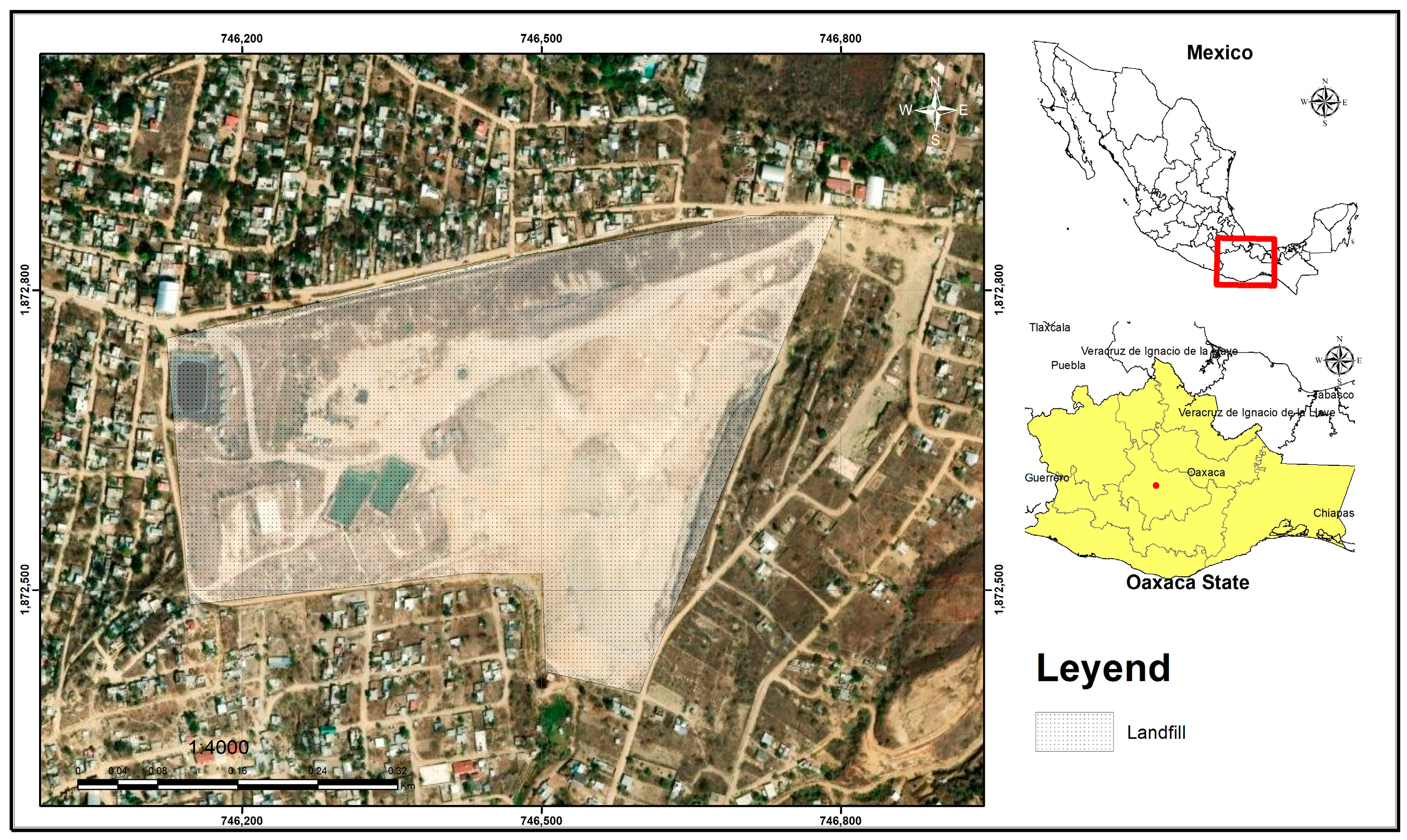
2.1. Study Area

The landfill is in the metropolitan area of Oaxaca de Juárez, Oaxaca, Mexico (Figure 1). Until 2022, this site was the main landfill operating for 24 municipalities since operations were stopped in the landfill due to social conflict. The landfill is a controlled site with an arrangement in confinement cells, so it has infrastructure for the collection and treatment of leachate. On site, the waste is compacted and covered by tractors and backhoe loaders. The area of the landfill is approximately 17.08 hectares [30].

2.2. Climatology

The temperature and precipitation data for Mexico were obtained from the climate change knowledge portal of the World Bank [31], and the same data series were obtained for the city of Oaxaca (Figure 2) from the weather station 20,022 (Coyotepec), which is located in San Bartolo Coyotepec, 5 km from the landfill [32]. The average annual temperature for the period from 1980 to 2010 was 20 °C, and the average annual precipitation (aap) was 484.8 mm. This information is necessary to calculate the constant rate of generation of CH₄ (k) and the potential of generation L₀ for mathematical models. In general, an important presence of precipitation is observed during the summer (an average value of 102.1 mm for June, July, and August) for the same period.

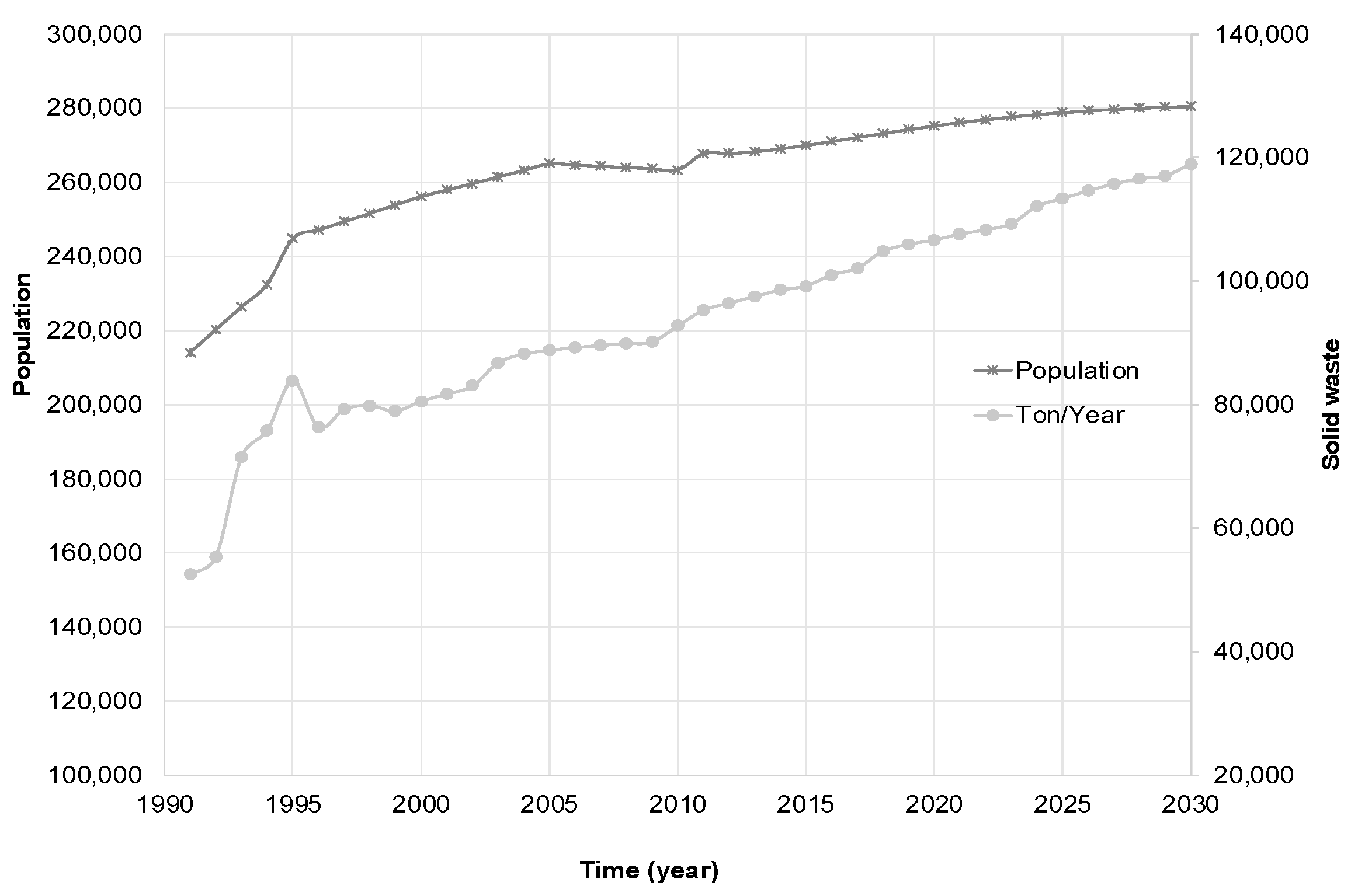
2.3. Population and Generation of Waste in the City of Oaxaca

Data on population growth and the generation of waste per day were obtained from the National Institute of Statistics and Geography [33] and the Organization for Cooperation and Economic Development [34]. The INEGI publishes data from the population census every 5 years for the period from 1990 to 2020, so interpolation was carried out to describe the yearly data. The available data for the generation of solid waste (Ton/year) correspond to the period from 1991 to 2012, whereby an extrapolation for the period from 2012 to 2021 was carried out via the FORECAST function in Excel. In 1991, 52,554.72 tons/year were reported, and in 2022, 108,202 tons/year were estimated (Figure 3).

Waste generation data are trended data series. This information is essential for predicting methane generation. An autoregressive integrative moving average model (ARIMA) was used to model these data. The ARIMA model is a statistical model with three parameters (p, d, and q) that is used to analyze time series. ARIMA models are used to make predictions while considering past data. An ARIMA model is structured with 3 parameters: p is the lag order; d is the degree of differencing; and q is the order of the moving average. The ARIMA model has the capacity to capture the patterns that exist in waste generation with respect to time. Importantly, ARIMA captures seasonality, trends, and remaining patterns.

According to [35], an ARIMA model can be defined as follows:

If d is a nonnegative integer, then $\left\{{\mathrm{X}}_{\mathrm{t}}\right\}$ is an ARIMA (p, d, q) process if Yt: = (1 − B ^dX_t is a causal ARMA (p, q) process.

This definition means that {X_t} satisfies a difference equation of the form:

$${\mathrm{\varnothing }}^{*}\left(\mathrm{B}\right){\mathrm{X}}_{\mathrm{t}}\equiv \mathrm{\varnothing }\left(\mathrm{B}\right){\left(1-\mathrm{B}\right)}^{\mathrm{d}}{\mathrm{X}}_{\mathrm{t}}=\mathsf{\theta }\left(\mathrm{B}\right){\mathrm{Z}}_{\mathrm{t}},\hspace{1em}\left\{{\mathrm{Z}}_{\mathrm{t}}\right\}~\mathrm{W}\mathrm{N}\left(0,{\mathsf{\sigma }}^2\right),$$

(1)

where $\mathrm{\varnothing }\left(\mathrm{z}\right)$ and $\mathsf{\theta }\left(\mathrm{z}\right)$ are polynomials of degrees p and q, respectively, and $\mathsf{\theta }\left(\mathrm{z}\right)\ne 0$ for $\left|\mathrm{z}\right|\le 1$. The polynomial ${\mathrm{\varnothing }}^{*}\left(\mathrm{z}\right)$ is of zero order at $\mathrm{z}=1$.

To analyze the waste generation data series, it is necessary to verify if a series is stationary; otherwise, the data must be differentiated. A systematic approach for testing the presence of a unit root of the autoregressive polynomial is possible by using the Dickey-Fuller test. This approach was proposed by [36,37] and is a single root test that statistically detects the presence of stochastic trend behavior in the time series of the variables by means of a hypothesis test.

According to [35], to verify the presence of a unit root, we can define it as follows:

Let X₁, …, X_n be observations from the AR (1) model.

$${\mathrm{X}}_{\mathrm{t}}-\mathsf{\mu }={\mathrm{\varnothing }}_1\left({\mathrm{X}}_{\mathrm{t}-1}-\mathsf{\mu }\right)+{\mathrm{Z}}_{\mathrm{t}},\left\{{\mathrm{Z}}_{\mathrm{t}}\right\}~\mathrm{W}\mathrm{N}\left(0,{\mathsf{\sigma }}^2\right)$$

(2)

where $\left|{\mathrm{\varnothing }}_1\right|<1$ and $\mathsf{\mu }={\mathrm{E}\mathrm{X}}_{\mathrm{t}}$. For large values of n, the maximum likelihood estimator ${\widehat{\mathrm{\varnothing }}}_1 \mathrm{o}\mathrm{f} {\mathrm{\varnothing }}_1$ is approximately $\mathrm{N}\left({\displaystyle \raisebox{1ex}{${\mathrm{\varnothing }}_1,\left(1-{\mathrm{\varnothing }}_1^2\right)$}\!\left/ \!\raisebox{-1ex}{$\mathrm{n}$}\right.}\right).$ For the unit root case, this normal approximation is no longer applicable, even asymptotically. This precludes its use for testing the unit root hypothesis ${\mathrm{H}}_0:{\mathrm{\varnothing }}_1=1 \mathrm{v}\mathrm{s}. {\mathrm{H}}_1:{\mathrm{\varnothing }}_1<1$. To construct a test of H₀, the model is written as

$$\nabla {\mathrm{X}}_{\mathrm{t}}={\mathrm{X}}_{\mathrm{t}}-{\mathrm{X}}_{\mathrm{t}-1}={\mathrm{\varnothing }}_0^{*}+{\mathrm{\varnothing }}_1^{*}{\mathrm{X}}_{\mathrm{t}-1}+{\mathrm{Z}}_{\mathrm{t}},\left\{{\mathrm{Z}}_{\mathrm{t}}\right\}~\mathrm{W}\mathrm{N}\left(0,{\mathsf{\sigma }}^2\right),$$

where ${\mathrm{\varnothing }}_0^{*}=\mathsf{\mu }\left(1-{\mathrm{\varnothing }}_1\right)$ and ${\mathrm{\varnothing }}_1^{*}={\mathrm{\varnothing }}_1-1.$ Now, let ${\widehat{\mathrm{\varnothing }}}_1^{*}$ be the ordinary least squares (OLS) estimator of ${\mathrm{\varnothing }}_1^{*}$ found by regressing $\nabla {\mathrm{X}}_{\mathrm{t}}$ on 1 and ${\mathrm{X}}_{\mathrm{t}-1}.$ The estimated standard error of ${\widehat{\mathrm{\varnothing }}}_1^{*}$ is shown in Equation (3):

$$\widehat{\mathrm{S}\mathrm{E}}\left({\widehat{\mathrm{\varnothing }}}_1^{*}\right)=\mathrm{S}{\left(\sum _{\mathrm{t}=2}^{\mathrm{n}}{\left({\mathrm{X}}_{\mathrm{t}-1}-\overline{\mathrm{X}}\right)}^2\right)}^{-{\displaystyle \raisebox{1ex}{$1$}\!\left/ \!\raisebox{-1ex}{$2$}\right.}}$$

(3)

The Dickey-Fuller test was implemented to analyze the waste generation data. The null hypothesis of the test states the existence of a unit root. The test statistic is compared with the corresponding critical value.

2.4. Volume of Waste

The volume of solid waste was estimated by using gravimetric measurements. Gravimetry is based on the study of subsurface properties by measuring and analyzing the gravity field at the Earth’s surface. This field is affected by the mass distributions and discontinuities of the subsurface, which are characterized by density [38]. Gravimetric anomalies are generated by variations in the density of various materials. These anomalies can be analyzed to identify deposits and subsurface structures and to estimate the volume of waste disposed of at the landfill.

Gravimetric measurements were performed on the mass of waste in the landfill. A Lacoste & Romberg G-247 gravimeter with a resolution of 10 µGa was used [39], with an average spacing between stations of 272 m. A total of 188 gravimetry data points measured at the height of the waste mass were used to implement spatial corrections for latitude, free air, and mass. The methodology proposed by [38] was used. The following equation was used to estimate the simple Bouguer anomaly:

$$g_{SBA}=g_{obs}-g_{\theta }+g_{h\theta }-g_m$$

(4)

where

g_SBA = Simple Bouguer gravity anomaly (mGal).

g_obs = Observed gravity (mGal).

$g_{\theta }$ = Correction for latitude (mGal).

$g_{h\theta }$ = Height correction or free air (mGal).

g_m = Bouguer correction (mGal).

The residual Bouguer anomaly was then calculated using Equation (5):

$$A_r=\mathsf{A}-A_R$$

(5)

where

A_r = Residual anomaly (mGal).

A = Gravity anomaly resulting from the reduction in observed gravity data (mGal).

A_R = Regional anomaly (mGal).

The Bouguer anomaly consists of the elimination of regional effects by large-scale geological structures. A first-order polynomial adjustment was used. From this difference, the residual Bouguer anomaly map was generated, and 6 profiles were plotted (Figure 4). A geological–geophysical model was used, which is a conceptual representation of geological data such as the stratigraphy and lithology of the area under study. The thicknesses and densities of the materials were considered according to geological chart E14-12 Zaachila Oaxaca [40]. According to this model, there is a shale–sandstone sedimentary rock layer and a metamorphic layer called gneiss (

Table 1. Material thicknesses and densities.

		Approximate Thickness (m)	Density (gr/cm3)	Reference
SDF Zaachila	Compacted mixed waste	6–64	0.445	[41]
Sedimentary	Sandstones–shales	15–78	2.1	[38]
Metamorphic	Gneiss	250	2.7	[38]

).

For modeling, the method proposed by [42,43,44] was implemented. With this method, irregular bodies can be represented by means of a polygonal section geometry.

With the information from the depth profiles along the Z axis, a thickness map was obtained. A meshing of 5 m × 5 m was used across the study area. Equation (6) was used to calculate the mass of waste deposited in the landfill.

$$\mathsf{{\rm M}}=\rho \ast V$$

(6)

where

M = Mass (kg).

$\mathsf{\rho }$ = Density (kg/m³).

V = Volume (m³).

2.5. Composition of Solid Waste

The composition of the MSW refers to the percentage of each subproduct that conforms to the total mass of the waste. The fraction of organic waste was 53%, and that of inorganic waste was 47% (

Table 2. Composition of solid waste.

Classification of Waste		Percentage (%)
Organic	Food waste	32.0
	Landscaping waste	10.2
	Paper	4.0
	Rag	3.5
	Cardboard	2.1
	Cotton	1.0
	Wood	0.1
Inorganic	Disposable diapers	11.4
	Fine residue	9.5
	Others	9.2
	Plastic	8.8
	Glass	3.4
	Rubber	1.6
	Tetrapack	1.1
	Cans	0.8
	Earthenware and ceramics	0.4
	Leather	0.2
	Iron	0.2
	Synthetic fibers	0.2
	Aluminum	0.1

); the composition was reported previously [6]. According to a study by the government of the state of Oaxaca, information is available on the percentages of each byproduct. Therefore, the amount of organic waste that influences the generation of methane can be determined. To group the percentages of organic waste, the IPCC guidelines were consulted [45].

2.6. Mathematical Models for Methane Emissions

The generation of biogas can be calculated using mathematical models according to the order of the reaction for decomposition of the organic matter [46]. These models of decay or decomposition can be classified into zero-order models, first-order models, second-order models, multiphase models, or a combination of orders. In this work, we are interested in applying first-order decay models, mainly due to data accessibility. Additionally, we choose 3 monophasic models and 2 multiphasic models to corroborate their predictive capacity. Increasing the order of the equation will require more parameters, which are difficult to measure at the site, and the complexity increases. The IPCC and LANDGEM models were included in this work; since they are the most applied methods, they are models of reference. On the other hand, first-order decay (FOD) models are based on two critical parameters: the methane generation potential (L₀), which depends on waste composition and its degradable organic content, and the CH₄ generation rate constant (k), which depends on waste composition, annual precipitation, and ambient temperature [47,48]. Data availability is crucial to implement the models; in this way, the proposed models can be solved for Zaachila’s landfill. The equations are described in

Table 3. First-order decay models.

Model	Equation	Index of Symbols
Simple of first order	$$\mathrm{G}=\mathrm{W}{\mathrm{L}}_0\mathrm{k}{\mathrm{e}}^{-\mathrm{k}\left(\mathrm{t}-{\mathrm{t}}_{\mathrm{i}}\right)}$$ (1) [23]	G = Generation of methane (m3/year) W = Mass of waste (Tons) L0 = Potential of generation of methane (m3/Ton) t = Time after waste placement (years) ti = Lag time (between placement and the start of generation k = First-order rate constant (year−1)
Simple of first order modified	$$\mathrm{G}=\mathrm{W}{\mathrm{L}}_0{\displaystyle \frac{\mathrm{k}+\mathrm{s}}{\mathrm{s}}}\left[1-{\mathrm{e}}^{-\mathrm{s}\left(\mathrm{t}-{\mathrm{t}}_{\mathrm{i}}\right)}\right]\left[\mathrm{k}{\mathrm{e}}^{-\mathrm{k}\left(\mathrm{t}-{\mathrm{t}}_{\mathrm{i}}\right)}\right]$$ (2) [23]	G = Generation of methane (m3/year) W = Mass of waste (Tons) L0 = Potential of generation of methane (m3/Ton) t = Time after waste placement (years) ti = Lag time (between placement and the start of generation k = First-order rate constant (year−1) s = Constant of the phase of first order
Multiphase model	$$\mathrm{G}=\mathrm{W}{\mathrm{L}}_{\mathrm{o}}\left[{\mathrm{F}}_{\mathrm{r}}\left({\mathrm{k}}_{\mathrm{r}}{\mathrm{e}}^{-{\mathrm{k}}_{\mathrm{r}}(\mathrm{t}-{\mathrm{t}}_{\mathrm{i}})}\right)+\left[{\mathrm{F}}_{\mathrm{s}}\left({\mathrm{k}}_{\mathrm{s}}{\mathrm{e}}^{{\mathrm{k}}_{\mathrm{r}}\left(\mathrm{t}-{\mathrm{t}}_{\mathrm{i}}\right)}\right)\right]\right]$$ (3) [23]	kr = Constant of decomposition of first order for rapidly decomposable waste ks = Constant of decomposition of first order for slowly decomposable waste Fr = Fraction of rapidly decomposable waste Fs = Fraction of slowly decomposable waste
LandGEM	$${\mathrm{Q}}_{{\mathrm{C}\mathrm{H}}_4}={\displaystyle \sum _{\mathrm{i}=1}^{\mathrm{n}}}{\displaystyle \sum _{\mathrm{j}=0.1}^1}\mathrm{k}{\mathrm{L}}_0\left({\displaystyle \frac{{\mathrm{M}}_{\mathrm{i}}}{10}}\right){\mathrm{e}}^{-\mathrm{k}{\mathrm{t}}_{\mathrm{i}\mathrm{j}}}$$ (4) [49]	QCH4 = Annual methane generation in the year of calculation (m3/year) n = (Year of the calculation)—(initial year of waste acceptance) i = 1 year time increment j = 0.1-year time increment k = Methane generation rate (year−1) L0 = Potential methane generation capacity (m3/Mg) Mi = Mass of waste accepted in the ith year (Mg) tij = Age of the jth section of waste mass accepted in the ith year (decimal of year)
IPCC	$${\mathrm{C}\mathrm{H}}_4\mathrm{E}\mathrm{m}\mathrm{i}\mathrm{s}\mathrm{s}\mathrm{i}\mathrm{o}\mathrm{n}\mathrm{s}=\left[{\displaystyle \sum _{\mathrm{x}}}{\mathrm{C}\mathrm{H}}_{4{\mathrm{g}\mathrm{e}\mathrm{n}\mathrm{e}\mathrm{r}\mathrm{a}\mathrm{t}\mathrm{e}\mathrm{d}}_{\mathrm{x},\mathrm{T}}}-{\mathrm{R}}_{\mathrm{T}}\right]\ast \left(1-{\mathrm{O}\mathrm{X}}_{\mathrm{T}}\right)$$ (4) $${\mathrm{Q}}_{\mathrm{C}\mathrm{H}4 \mathrm{g}\mathrm{e}\mathrm{n}\mathrm{e}\mathrm{r}\mathrm{a}\mathrm{t}\mathrm{e}\mathrm{d} \mathrm{T}}={\mathrm{D}\mathrm{D}\mathrm{O}\mathrm{C}}_{\mathrm{m} \mathrm{d}\mathrm{e}\mathrm{c}\mathrm{o}\mathrm{m}\mathrm{p}\left(\mathrm{T}\right)}.\mathrm{F}\times \left({\displaystyle \frac{16}{12}}\right)$$ (5) $${\mathrm{D}\mathrm{O}\mathrm{C}}_{\mathrm{m} \mathrm{d}\mathrm{e}\mathrm{c}\mathrm{o}\mathrm{m}\mathrm{p}\left(\mathrm{T}\right)}={\mathrm{D}\mathrm{D}\mathrm{O}\mathrm{C}}_{\mathrm{m}\mathrm{a}\left(\mathrm{T}-1\right)}\times \left(1-{\mathrm{e}}^{-\mathrm{k}}\right)$$ (6) $${\mathrm{D}\mathrm{D}\mathrm{O}\mathrm{C}}_{\mathrm{m}\mathrm{a}\left(\mathrm{T}\right)}={\mathrm{D}\mathrm{D}\mathrm{O}\mathrm{C}}_{\mathrm{m}\mathrm{d}\left(\mathrm{T}\right)}+\left({\mathrm{D}\mathrm{D}\mathrm{O}\mathrm{C}}_{\mathrm{m}\mathrm{a}(\mathrm{T}-1)}\times {\mathrm{e}}^{-\mathrm{k}}\right)$$ (7) $${\mathrm{D}\mathrm{D}\mathrm{O}\mathrm{C}}_{\mathrm{m}}=\mathrm{W}\times \mathrm{D}\mathrm{O}\mathrm{C}\times {\mathrm{D}\mathrm{O}\mathrm{C}}_{\mathrm{f}}\times \mathrm{M}\mathrm{F}\mathrm{C}$$ (8) [45]	CH4 Emissions = CH4 emitted in the year T, Gg T = Inventory year X = Waste category or type/material RT = Recovered CH4 in year T, Gg OXT = Oxidation factor in year T (fraction) F = Fraction of CH4, by volume, in generated landfill gas (fraction) 16/12 = Ratio of molecular weight of CH4/C DDOCma(T) = DDOCm accumulated at the end of year T, Gg DDOCma(T-1) = DDOCm accumulated at the end of year (T-1), Gg DDOCmd(T) = DDOCm deposited in year T, Gg DDOCm decompT = DDOCm decomposed in the SWDS in year T, Gg k = Reaction constant (year—1) DDOCm = Total mass of degradable organic carbon (DDOC) in the year T W = Mass of waste deposited (Gg) DOC = Degradable organic carbon in the year of deposition, fraction, Gg C/Gg waste DOCf = Fraction of DOC that can decompose (fraction) MFC = CH4 correction factor for aerobic decomposition in the year of deposition (fraction)

.

2.7. Input Parameters of the Models

k and L₀ were calculated as functions of the specific conditions of the site, that is, by considering the average ambient conditions in the geographic zone and the waste composition. The value of k refers to the rate of degradation of the waste, and it can be affected by different variables, such as the pH, temperature, size of the particles, and moisture content [50]. Each component of the solid waste degrades at a different rate. The values of k reported in the literature range from 0.01 to 0.21 year⁻¹ [46] and can be calculated by the following equation:

$$\mathrm{k}={3.2\times 10}^{-5}\left(\mathrm{x}\right)+0.01$$

(7)

where x = average annual precipitation (mm).

Annual precipitation is often used as a substitute for moisture in waste because of the lack of information about the moisture conditions inside a landfill [49]. This parameter considers the average annual precipitation of the station nearest to the landfill, which is 484.8 mm/year.

The value of the potential generation of methane (L₀) is a function of the nature of the waste. Each component of the waste has a different degradation time since the content of organic carbon degradable (DOC) is different. According to the EPA (2008), the values of L₀ vary from 6 to 270 m³/Mg, and a predetermined value of 100 m³/Mg data was obtained from experimental studies in 40 landfills [51].

In our work, the value of L₀ was estimated according to the directives of the IPCC (Intergovernmental Panel on Climate Change) using the following equation [45]:

$${\mathrm{L}}_0=\mathrm{D}\mathrm{O}\mathrm{C}\times {\mathrm{D}\mathrm{O}\mathrm{C}}_{\mathrm{F}}\times \mathrm{F}\times {\displaystyle \frac{16}{12}} \times \mathrm{M}\mathrm{C}\mathrm{F}$$

(8)

where

DOC: Degradable organic carbon.

DOC_F = Fraction of the DOC that can degrade (%).

F = Fraction of methane generated in biogas (%).

16/12: Ratio of the molecular weight CH₄/C.

MCF: Methane correction factor.

2.7.1. Degradable Organic Carbon (DOC)

This corresponds to the organic carbon that degrades under anaerobic conditions in landfills. It is based on the composition of the waste and was estimated with the equation proposed by the IPCC [52].

$$DOC=0.4A+0.17B+0.15C+0.03 D$$

(9)

where

A: The fraction of MSW that corresponds to paper and textile waste.

B: The fraction of MSW that corresponds to garden and park waste.

C: The fraction of MSW that corresponds to food waste.

D: The fraction of MSW that corresponds to wood or straw.

The fraction of degradable organic carbon DOCf

The guidelines of the IPCC propose a standard value of 0.77. This parameter was estimated by considering the temperature of the anaerobic zone of the site, which is related to the reactions of degradation by microbial activity. The IPCC model proposes a temperature of 35 °C since it considers that the temperature in the anaerobic zone of landfills remains constant. Additionally, this fraction can be calculated from the following equation [53]:

$${DOC}_f=0.014T+0.28$$

(10)

where T = temperature in the anaerobic zone of the site (°C).

2.7.2. Fraction of CH₄ in Biogas

According to the guidelines of the IPCC, the fraction of methane in biogas is 50%, and the other 50% corresponds to CO₂. Therefore, this fraction is 0.5.

2.7.3. Ratio of Molecular Weight

This refers to the ratio of the molecular weight of methane (CH₄ = 16) and the molecular weight of the carbon (C = 12; 16/12), which is used to convert carbon to methane.

2.7.4. Methane Correction Factor (MCF)

This factor is related to the conditions of operation of the site. For the studied site, mechanical compaction is usually conducted, and a value of 1.0 is considered (

Table 4. Methane correction factor (MCF).

Type of Site	Default Values of MCF
Managed—anaerobic	1.0
Managed—semiaerobic	0.5
Not managed—deep (>5 m of waste and/or high-water table)	0.8
Not managed—shallow (<5 m of waste)	0.4
No category	0.6

).

Assumptions of the models:

Solid waste corresponds to municipal solid waste.

The site works under anaerobic conditions.

The waste composition remained constant throughout the study period.

3. Results

3.1. Volume of Waste

According to [54], the gravimetric method can be used to investigate the internal structure of a landfill. Figure 4 shows the values of the residual Bouguer anomaly and the calculated profiles. The Bouguer anomaly is the gravity anomaly and corresponds to the difference between the observed and theoretical gravity at an observation site. Profiles A, B, and C have a west-to-east orientation and lengths of 0.64, 0.57, and 0.51 km, respectively. Profiles D, E, and F have north-south orientations and lengths of 0.28, 0.30, and 0.43 km, respectively. The residual anomalies vary from −1.96 to 2.64 mGals. Low gravimetric values are found in the central part of the landfill (shades in purple), indicating that a mass deficiency exists in that area. Gravimetric highs represent an excess mass.

Figure 5 shows the depth map (z), which has a minimum value of 4 m and a maximum value of 53 m (average of 28 m). This information coincides with the data published in [30], which used vertical electrical soundings. These authors mention that thicknesses range from 6 to 64 m, which coincides with our information obtained by gravimetry. The greatest depths are observed in the central part of the site and are represented by blue shading, which coincides with the values where the residual anomaly map shows gravimetric lows, indicating that these depths are associated with greater waste deposits.

The calculation of the volume was performed from the calculated depths, values that were multiplied by the area of each cell in the grid (25 m²). The total calculated volume was 5,500,593.0 m³, with a mass of 2,451,504.2 tons.

3.2. Parameters k and L₀

In this work, we calculated k = 0.026 year⁻¹ by applying Equation (16), which considers the average annual precipitation, whereas the EPA propose a standard value of 0.02 year⁻¹ [49]. Escamilla et al. [29] suggested a value of k = 0.04 year⁻¹ for the same region. The climatic conditions affect the values for this parameter [55]. The variability of the value of k depends mainly on the average annual precipitation, which varies significantly across regions [48]. For this reason, it is important to use data from weather stations near the landfills.

For L₀, a value of 106 m³/Mg was calculated by following the IPCC methodology with Equations (17) and (18). The calculated values are shown in

Table 5. Data to calculate L₀.

Data	Values
Degradable organic carbon (DOC)	0.129
Fraction of degradable organic carbon DOCf	0.77
Fraction of CH4 in biogas	0.5
Ratio of molecular weight	1.33
Methane correction factor (MFC)	1
Density of methane at constant temperature	0.627 kg/m3

. The EPA proposed a standard value of 100 m³/Mg [49], and [29] proposed a value of 90.71 m³/Mg. It is well known that the value of L₀ is affected by the percentage of waste [55]. The value calculated in the present work is within the range suggested by the EPA (6–270 m³/Mg). For Latin America, the following values have been proposed: 69–200 m³/Mg for Colombia; 70, 96, and 200 m³/Mg for Costa Rica; 71, 89, and 198 m³/Mg for Guatemala; and 69–202 m³/Mg for Mexico [56].

3.3. Modeling Solid Waste Generation

The critical values of the Dickey-Fuller test showed a coefficient of −0.99, a standard error of 0.13, and a t statistic of −7.70. The critical values for 1% without trend = −3.43, and with trend = −3.96, and for 5%, the values were −2.86 and −3.41, respectively. The value of tau (−7.7017) was lower than the Dickey-Fuller critical value (for both with and without a trend), thus affirming the existence of a unit root.

Figure 6 shows the results of the prediction of the generation of residuals from the ARIMA model. The fact that the model considers data from the past allows us to describe the perturbations that may occur in the temporal information. In approximately 1995, an increase in waste generation was reported, which was correctly described by the model. During the period 2000–2020, an increase of approximately 27,000 tons of waste was observed, and by 2030, a generation of 120,000 tons/year was predicted. This waste generation is important for the estimation of methane generation. This model represents an accurate description of the time-series data and is considered for the calculation of emissions.

The ARIMA model is represented by the following equation:

$$\mathrm{Y}=8926.0716+\left(0.922545·{\mathrm{Y}}_{\mathrm{t}-1}\right)+49.1676+(-0.072215·\mathrm{e}\mathrm{r}\mathrm{r}\mathrm{o}\mathrm{r}) \left(\mathrm{t}\mathrm{o}\mathrm{n}\mathrm{s}\right)$$

We observed good predictive ability of the model by considering the range of values of waste generation. Additionally, (Figure 6) presents the values of the error.

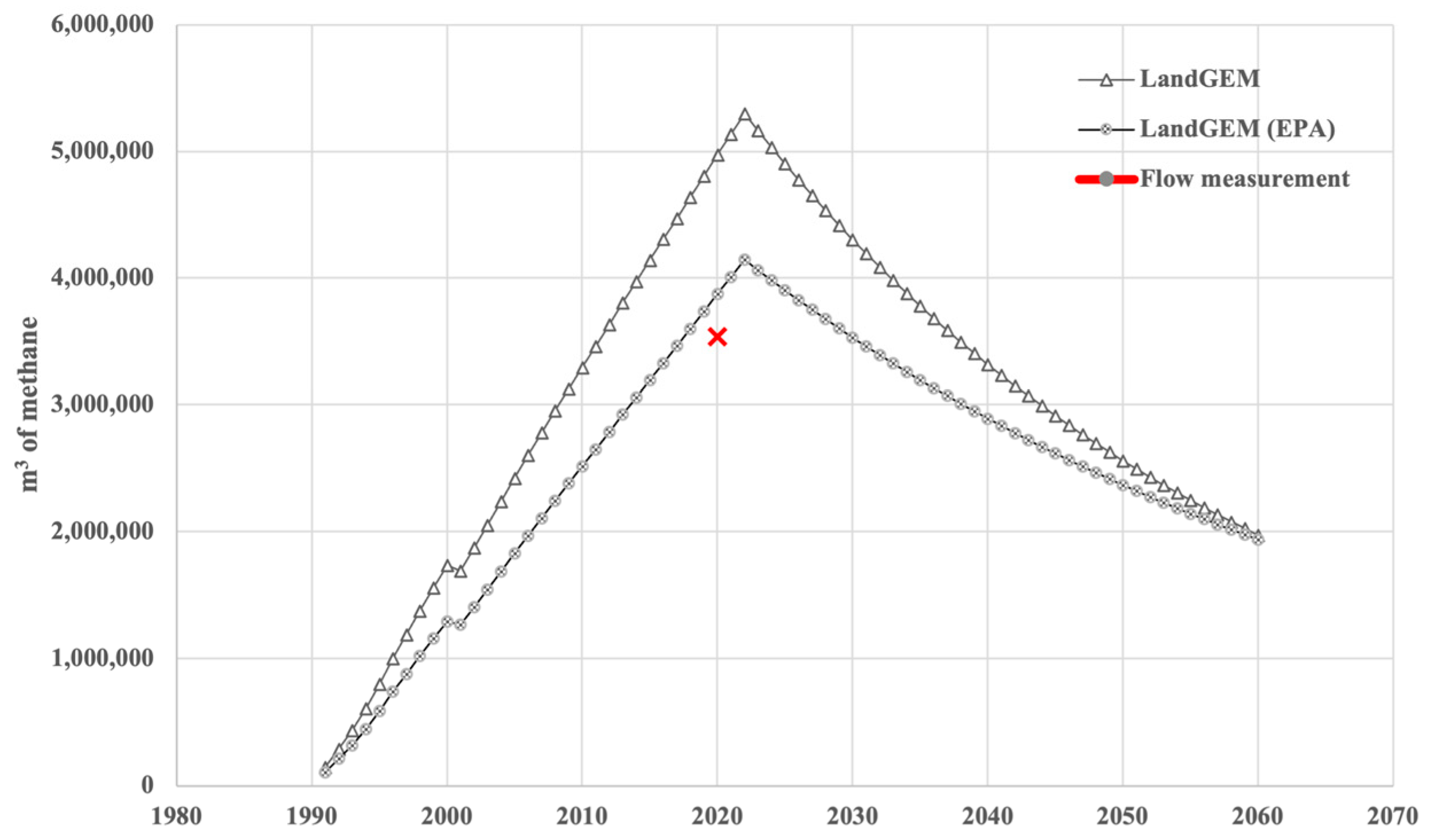
3.4. Modeling the Generation of Methane

Figure 7 shows the volume of generation of CH₄ by the five proposed models. The behavior of the curves reveals the generation of methane and its subsequent decay. A maximum of generation was observed, and then a decay occurred in several decades. The importance of calculating these emissions is related to the difficulty of experimentally measuring the generation of gases in landfills.

The difficulty in validating landfill methane generation models is also related to the limited experimental data. Figure 7 also shows one experimental value obtained in the landfill by the company “Sistemas de Ingeniería y Control Ambiental S.A. de C.V”. Flow sampling was performed at the heads of the biogas extraction wells. In 2020, this company measured the biogas flow in the headers of the extraction system. The behavior of the curves is consistent with the waste decomposition process, and overall, the five models correctly represent the methane generation process linked to waste decomposition.

According to this information, 7.14 × 10⁶ m³ of biogas was emitted in 2020 (at 1 atm and an average ambient temperature of 20 °C), of which 49.5% corresponded to methane, i.e., 3.53 × 10⁶ m³. These data allowed us to calculate the relative error (

Table 6. Relative errors for the models.

Model	m3/Year of CH4 in Year 2020	Relative Error (%)
Simple of first order	3.50 × 106	1.0
Simple of first order modified	3.76 × 106	6.3
Multiphase model	3.09 × 106	12.6
LandGEM	4.97 × 106	40.7
IPCC	3.19 × 106	9.7
Flow measurement (experimental)	3.53 × 106	-

) for each model. The simple and modified simple models presented the lowest errors (1% and 6.3%, respectively).

A comparison of the results revealed that the models with greater accuracy were the simple model and the modified simple model. These results coincide with those reported by [57], who reported that, compared with multiphase models, single-phase models effectively predict methane generation. Importantly, the multiphase model and IPCC consider different methane generation rates (k) for different waste categories, with underestimated results compared with the flux measurement in 2020 (Figure 7).

On the one hand, the multiphase model involves two processes that affect the equation: slow and fast degradation mechanisms, and on the other hand, the IPCC model considers methane generation rates (k) for each waste category. These effects can explain the deviation of the calculated results from the measured values. According to [57,58], models such as LandGEM may not be able to predict methane generation from landfills with heterogeneous wastes. This would explain the pronounced deviation of the LandGEM model in Figure 7, which also agrees with the work of Da Silva et al. [24].

Since the LandGEM model was the one that showed the greatest error, we proceeded to revise its parameters. In Figure 8, the k and Lo parameters were calculated according to the climatology and available information of composition for this landfill. A second calculation was conducted by considering the standard values suggested by the EPA [46,51]. The EPA proposed values of k = 0.02 and L₀ = 100 m³/Mg, so these values were considered in a second calculation. Figure 8 shows a new estimation for the LandGEM model, and we observe that the prediction was improved since the relative error was reduced to 9.6%.

All the models estimate important methane emissions for the next 30 years. In the case of the simple and modified simple models, for the year 2050, emissions of 1.22 × 10⁶ m³ and 1.37 × 10⁶ m³ of methane are estimated. Importantly, this volume can be affected by environmental conditions and biological activity in landfills in the next few years [16,59]. In [60], the authors affirm that the stabilization of emissions depended on several factors; however, the authors suggested that these periods can vary in the range of 10, 15, and up to 30 years. These authors reported that emissions depend on the climatic area; for example, for humid areas, periods vary from 2 to 5 years, and for dry areas, periods vary from 10 to 25 years. Similarly, according to [61], the duration and composition of biogas in a landfill depend on the stage of decomposition.

It is important to note the numerical difference between the models. Figure 7 shows the differences in the quantities calculated by each model. This fact has also been observed in different studies [15,24], which reveal the difficulty of accurately predicting such gaseous emissions. On the one hand, the estimation of emissions in landfills is very difficult because of the complexity of the variables and mechanisms that affect these processes. On the other hand, large amounts of experimental data and several years of experimental monitoring are needed to validate the models. For example, in the work of [18], the authors applied five prediction models for biogas generation in two landfills in Argentina. The studied models were the LandGEM, IPCC, AMS, and Mexican models and the model for China. The authors mention that the LandGEM model gave better results, but they compared only three experimental measurements, which corresponded to the years 2006, 2007, and 2008. The models revealed significant differences, with biogas rates of up to 8000 m³/h. The differences are linked to the uncertainty of the main model parameters, such as waste characterization, and the site management factor. Likewise, leachate management and compaction techniques can affect the results, as well as the characterization of waste and the quantities discharged per day. These aspects cause deficiencies in external sealing, resulting in the presence of fugitive emissions or aerobic processes. In addition, failure in compaction and sealing procedures can affect the aerobic processes produced during the waste decomposition stage. One way to improve model prediction would be to ensure adequate compaction levels, maintain periodic coverage, and control potential fugitive emissions; nevertheless, extensive experimental monitoring is needed.

4. Conclusions

The analysis and processing of gravimetric anomalies allowed for the identification of variations in the waste deposits in the landfill, which determined areas of greater accumulation of solid waste. The usefulness of this method in the characterization of landfills is highlighted since it allows us to estimate the volume and mass of accumulated waste.

The implementation of the ARIMA model was useful for obtaining a time series of solid waste generation data. These data are among the input data for the application of first-order decay models. The prediction obtained with the application of first-order models for methane generation should be validated in the future. The five models exhibited decay behavior over time, considering that waste was no longer disposed of due to closure. However, quantitative differences between the models were identified because of the complex nature of the phenomena involved. In this research, the simple model and modified model yielded values close to the 2020 measurement values.

Moreover, with methane emission prediction models, long-term environmental impacts can be measured since, even though a decade has passed since the last disposal of waste in the landfill, it continues to emit large amounts of methane, which demonstrates the continued contribution of this site to environmental liability. The projections obtained for the year 2050 underscore the need to implement technologies to reduce methane emissions or their feasibility of use.

The development of predictive models faces challenges in modeling and monitoring because of the interaction of multiple factors, such as soil permeability, leachate management, and fugitive emissions. Our study reveals the importance of combining the application of mathematical models with practical strategies such as impermeable covers and biogas capture systems in landfills. To address the limitations and validation of model prediction, we identified the importance of further investment in instrumentation for long-term monitoring and experimental studies in Oaxaca city. This manuscript reveals relevant information for planning methane mitigation strategies. The latter is critical since Mexico joined the Global Methane Initiative in 2004.

References

1. Loganath, R.; Mohammed Bin Zacharia, K.; Kumar, A.; Singh, E.; Varma, V.S.; Sharma, D. System optimization models for solid waste management. In Current Developments in Biotechnology and Bioengineering; Elsevier: Amsterdam, The Netherlands, 2021; pp. 349–371. ISBN 978-0-12-821009-3. [Google Scholar] [CrossRef]
2. Kaza, S.; Yao, L.C.; Bhada-Tata, P.; Van Woerden, F. What a Waste 2.0: A Global Snapshot of Solid Waste Management to 2050; World Bank: Washington, DC, USA, 2018; ISBN 978-1-4648-1329-0. [Google Scholar] [CrossRef]
3. Kua, H.W.; He, X.; Tian, H.; Goel, A.; Xu, T.; Liu, W.; Yao, D.; Ramachandran, S.; Liu, X.; Tong, Y.W.; et al. Life cycle climate change mitigation through next-generation urban waste recovery systems in high-density Asian cities: A Singapore Case Study. Resour. Conserv. Recycl. 2022, 181, 106265. [Google Scholar] [CrossRef]
4. Paes, M.X.; De Medeiros, G.A.; Mancini, S.D.; Gasol, C.; Pons, J.R.; Durany, X.G. Transition towards eco-efficiency in municipal solidwaste management to reduce GHG emissions: The case of Brazil. J. Clean. Prod. 2020, 263, 121370. [Google Scholar] [CrossRef]
5. Kumar, A.; Sharma, M.P. Estimation of GHG emission and energy recovery potential from MSW landfill sites. Sustain. Energy Technol. Assess. 2014, 5, 50–61. [Google Scholar] [CrossRef]
6. Gobierno del Estado de Oaxaca. Resumen Ejecutivo del Programa Estatal Para la Prevención y Gestión Integral de los Residuos Sólidos Urbanos y de Manejo Especial en el Estado de Oaxaca; Secretaria de Medio Ambiente Energías y Desarrollo Sustentable, Oaxaca: Oaxaca, Mexico, 2013; Available online: https://www.oaxaca.gob.mx/semaedeso/wp-content/uploads/sites/59/2022/08/Resumen-Ejecutivo-PEPGIRSUME.pdf (accessed on 25 November 2024).
7. SEMARNAT. Diagnóstico Básico Para la Gestión Integral de los Residuos Sólidos. Mexico, 2020. Secretaria de Medio Ambiente y Recursos Naturales, México. 2020. Available online: https://www.gob.mx/cms/uploads/attachment/file/554385/DBGIR-15-mayo-2020.pdf (accessed on 25 November 2024).
8. Rueda-Avellaneda, J.F.; Rivas-García, P.; Gomez-Gonzalez, R.; Benitez-Bravo, R.; Botello-Álvarez, J.E.; Tututi-Avila, S. Current and prospective situation of municipal solid waste final disposal in Mexico: A spatio-temporal evaluation. Renew. Sustain. Energy Transit. 2021, 1, 100007. [Google Scholar] [CrossRef]
9. Kumar, S.; Nimchuk, N.; Kumar, R.; Zietsman, J.; Ramani, T.; Spiegelman, C.; Kenney, M. Specific model for the estimation of methane emission from municipal solid waste landfills in India. Bioresour. Technol. 2016, 216, 981–987. [Google Scholar] [CrossRef]
10. Molina, L.; Puentes, A.; Ortuzar, F.; Zirath, S.; Islas, I.; Gonzalez, R.; Masera, O.; Bickel, J.; Ortinez, A.; Castelan-Ortega, O.; et al. Avances y Oportunidades en la Reducción de Contaminantes Climáticos de Vida Corta en América Latina y el Caribe; UN Environment: Nairobi, Kenya, 2018. [Google Scholar]
11. Malmir, T.; Lagos, D.; Eicker, U. Optimization of landfill gas generation based on a modified first-order decay model: A case study in the province of Quebec, Canada. Environ. Syst. Res. 2023, 12, 6. [Google Scholar] [CrossRef]
12. MathWorks What Is the Genetic Algorithm? Available online: https://la.mathworks.com/help/gads/what-is-the-genetic-algorithm.html?lang=en (accessed on 25 November 2024).
13. Mir, A.A.; Mushtaq, J.; Dar, A.Q.; Patel, M. A quantitative investigation of methane gas and solid waste management in mountainous Srinagar city-A case study. J. Mater. Cycles Waste Manag. 2023, 25, 535–549. [Google Scholar] [CrossRef]
14. Pheakdey, D.V.; Noudeng, V.; Xuan, T.D. Landfill Biogas Recovery and Its Contribution to Greenhouse Gas Mitigation. Energies 2023, 16, 4689. [Google Scholar] [CrossRef]
15. Amini, H.R.; Reinhart, D.R.; Niskanen, A. Comparison of first-order-decay modeled and actual field measured municipal solid waste landfill methane data. Waste Manag. 2013, 33, 2720–2728. [Google Scholar] [CrossRef]
16. Thompson, S.; Sawyer, J.; Bonam, R.; Valdivia, J.E. Building a better methane generation model: Validating models with methane recovery rates from 35 Canadian landfills. Waste Manag. 2009, 29, 2085–2091. [Google Scholar] [CrossRef]
17. Colomer Mendoza, F.J.; García Darás, F.; Esteban Altabella, J.; Robles Martínez, F.; Aranda, G. Emisiones gaseosas de un relleno sanitario en México. Comparación con modelos de generación de biogás. Rev. Int. Contam. Ambie. 2016, 32, 113–122. [Google Scholar] [CrossRef]
18. Córdoba, V.; Blanco, G.; Santalla, E.M. Modelado de la generación de biogás en rellenos sanitarios. Av. En Energías Renov. Y Medio Ambiente 2009, 13, 69–76. [Google Scholar]
19. NOAA Global Monitoring Laboratory—Carbon Cycle Greenhouse Gases. Available online: https://gml.noaa.gov/ccgg/trends_ch4/ (accessed on 27 July 2023).
20. Kuylenstierna, J.C.; Michalopoulou, E.; Malley, C. Global Methane Assessment: Benefits and Costs of Mitigating Methane Emissions. Available online: http://www.unep.org/resources/report/global-methane-assessment-benefits-and-costs-mitigating-methane-emissions (accessed on 14 February 2024).
21. Bouyakhsass, R.; Souabi, S.; Bouaouda, S.; Taleb, A.; Kurniawan, T.A.; Liang, X.; Goh, H.H.; Anouzla, A. Adding value to unused landfill gas for renewable energy on-site at Oum Azza landfill (Morocco): Environmental feasibility and cost-effectiveness. Trends Food Sci. Technol. 2023, 142, 104168. [Google Scholar] [CrossRef]
22. Chandrasekaran, R.; Busetty, S. Estimating the methane emissions and energy potential from Trichy and Thanjavur dumpsite by LandGEM model. Environ. Sci. Pollut. Res. 2022, 29, 48953–48963. [Google Scholar] [CrossRef] [PubMed]
23. Vogt, W.G.; Augenstein, D. Comparison of Models for Predicting Landfill Methane Recovery; Final Report(NREL/SR--430-26041); Institution for Environmental Management: Palo Alto, CA, USA, 1997; p. 314088. [Google Scholar] [CrossRef]
24. Da Silva, N.F.; Schoeler, G.P.; Lourenço, V.A.; De Souza, P.L.; Caballero, C.B.; Salamoni, R.H.; Romani, R.F. First order models to estimate methane generation in landfill: A case study in south Brazil. J. Environ. Chem. Eng. 2020, 8, 104053. [Google Scholar] [CrossRef]
25. Nzotungicimpaye, C.-M.; MacIsaac, A.J.; Zickfeld, K. Delaying methane mitigation increases the risk of breaching the 2 °C warming limit. Commun. Earth Environ. 2023, 4, 250. [Google Scholar] [CrossRef]
26. United Nations Environment Program Methane Emissions are Driving Climate Change. Here’s How to Reduce Them. Available online: https://www.unep.org/news-and-stories/story/methane-emissions-are-driving-climate-change-heres-how-reduce-them (accessed on 21 November 2024).
27. Secretaria de Relaciones Exteriores México se Adhirió al Compromiso Global de Metano en la COP26, gob.mx. Available online: http://www.gob.mx/sre/prensa/mexico-se-adhirio-al-compromiso-global-de-metano-en-la-cop26?state=published (accessed on 21 November 2024).
28. Observatorio Mexicano de Emisiones de Metano Petróleo y Gas, Observatorio Mexican. Available online: https://www.obmem.mx/sector-petroleo-y-gas-mx (accessed on 21 November 2024).
29. Escamilla-García, P.E.; Jiménez-Castañeda, M.E.; Fernández-Rodríguez, E.; Galicia-Villanueva, S. Feasibility of energy generation by methane emissions from a landfill in southern Mexico. J. Mater. Cycles Waste Manag. 2020, 22, 295–303. [Google Scholar] [CrossRef]
30. Garrido, P.A.L.; Gómez, J.S. Saneamiento del tiradero de la ciudad de Oaxaca de Juárez. In Revista AIDIS de Ingeniería y Ciencias Ambientales. Investigación, Desarrollo y Práctica; Instituto de Ingeniería, Universidad Nacional Autónoma de México: Mexico City, Mexico, 2006; Available online: https://www.revistas.unam.mx/index.php/aidis/article/view/14440 (accessed on 6 February 2024).
31. CCKP World Bank Climate Change Knowledge Portal. Available online: https://climateknowledgeportal.worldbank.org/ (accessed on 14 February 2024).
32. CONAGUA Climogramas 1981–2010. Available online: https://smn.conagua.gob.mx/es/climatologia/informacion-climatologica/climogramas-1981-2010 (accessed on 8 February 2024).
33. INEGI Banco de Indicadores. Available online: https://www.inegi.org.mx/app/indicadores/ (accessed on 30 December 2023).
34. OECD Waste—Municipal Waste. Available online: http://data.oecd.org/waste/municipal-waste.htm (accessed on 30 December 2023).
35. Brockwell, P.J.; Davis, R.A. Introduction to Time Series and Forecasting; Springer Texts in Statistics; Springer International Publishing: Cham, Switzerland, 2016; ISBN 978-3-319-29852-8. [Google Scholar] [CrossRef]
36. Dickey, D.; Fuller, W. Distribution of the Estimators for Autoregressive Time Series With a Unit Root. JASA J. Am. Stat. Assoc. 1979, 74, 427–431. [Google Scholar] [CrossRef]
37. Dickey, D.G. Dickey-Fuller Tests. In International Encyclopedia of Statistical Science; Lovric, M., Ed.; Springer: Berlin/Heidelberg, Germany, 2011; pp. 385–388. ISBN 978-3-642-04898-2. [Google Scholar] [CrossRef]
38. Hinze, W.J.; Von Frese, R.R.B.; Saad, A.H. Gravity and Magnetic Exploration: Principles, Practices, and Applications; Cambridge University Press: Cambridge, UK, 2013; ISBN 978-0-521-87101-3. [Google Scholar]
39. LaCoste & Romberg Instruction Manual; Micro g LaCoste: Lafayette, CO, USA, 2004; Available online: https://microglacoste.com/support/product-manuals/ (accessed on 17 April 2024).
40. SGM Carta Geológico-Minera Zaachila E14-12, Oaxaca, Esc. 1:250,000. Available online: https://mapserver.sgm.gob.mx/Cartas_Online/metadatos_geol/100_GL_zaachila.html (accessed on 5 January 2024).
41. Tchobanoglous, G.; Theissen, H.; Eliassen, R. Desechos Sólidos Principios de Ingeniería y Administración. in Ambiente y los Recursos Naturales Renovables, no. AR-16. Venezuela, 1982. Available online: https://www.passeidireto.com/es/content/115360937/desechos-solidos-principios-de-ingenieria-y-administracion-2 (accessed on 28 July 2023).
42. Talwani, M.; Worzel, J.L.; Landisman, M. Rapid gravity computations for two-dimensional bodies with application to the Mendocino submarine fracture zone. J. Geophys. Res. (1896–1977) 1959, 64, 49–59. [Google Scholar] [CrossRef]
43. İşseven, T.; Aydın, N.G.; Arslan, M.S. 2D modelling the depth of the southeastern Thrace Basin by using Bouguer gravity anomalies. Acta Geophys. 2024, 72, 849–860. [Google Scholar] [CrossRef]
44. Mohammed, M.A.A.; Mohammed, S.H.; Szabó, N.P.; Szűcs, P. Geospatial modeling for groundwater potential zoning using a multi-parameter analytical hierarchy process supported by geophysical data. Discov. Appl. Sci. 2024, 6, 121. [Google Scholar] [CrossRef]
45. IPCC Directrices del IPCC de 2006 Para los Inventarios Nacionales de Gases de Efecto Invernadero 3.1. Available online: https://www.ipcc-nggip.iges.or.jp/public/2006gl/spanish/vol5.html (accessed on 28 July 2023).
46. Amini, H.R.; Reinhart, D.R.; Mackie, K.R. Determination of first-order landfill gas modeling parameters and uncertainties. Waste Manag. 2012, 32, 305–316. [Google Scholar] [CrossRef]
47. Machado, S.L.; Carvalho, M.F.; Gourc, J.-P.; Vilar, O.M.; do Nascimento, J.C.F. Methane generation in tropical landfills: Simplified methods and field results. Waste Manag. 2009, 29, 153–161. [Google Scholar] [CrossRef] [PubMed]
48. Park, J.-K.; Chong, Y.-G.; Tameda, K.; Lee, N.-H. Methods for Determining the Methane Generation Potential and Methane Generation Rate Constant for the FOD Model: A Review. Waste Manag. Research 2018, 36, 200–220. [Google Scholar] [CrossRef]
49. EPA Visualización de Documentos|NEPIS|EPA de EE. UU. Available online: https://nepis.epa.gov/Exe/ZyNET.exe/P1009C8L.txt?ZyActionD=ZyDocument&Client=EPA&Index=2016%20Thru%202020%7C1991%20Thru%201994%7C2011%20Thru%202015%7C1986%20Thru%201990%7C2006%20Thru%202010%7C1981%20Thru%201985%7C2000%20Thru%202005%7C1976%20Thru%201980%7C1995%20Thru%201999%7CPrior%20to%201976%7CHardcopy%20Publications&Docs=&Query=600r05047&Time=&EndTime=&SearchMethod=2&TocRestrict=n&Toc=&TocEntry=&QField=&QFieldYear=&QFieldMonth=&QFieldDay=&UseQField=&IntQFieldOp=0&ExtQFieldOp=0&XmlQuery=&File=D%3A%5CZYFILES%5CINDEX%20DATA%5C00THRU05%5CTXT%5C00000026%5CP1009C8L.txt&User=ANONYMOUS&Password=anonymous&SortMethod=h%7C-&MaximumDocuments=15&FuzzyDegree=0&ImageQuality=r85g16/r85g16/x150y150g16/i500&Display=hpfr&DefSeekPage=x&SearchBack=ZyActionL&Back=ZyActionS&BackDesc=Results%20page&MaximumPages=1&ZyEntry=1&SeekPage=x (accessed on 7 January 2024).
50. Faour, A.A.; Reinhart, D.R.; You, H. First-order kinetic gas generation model parameters for wet landfills. Waste Manag. 2007, 27, 946–953. [Google Scholar] [CrossRef] [PubMed]
51. EPA Background Information Document for Updating AP42 Section 2.4 for Estimating Emissions from Municipal Solid Waste Landfills|Science Inventory|US EPA. Available online: https://cfpub.epa.gov/si/si_public_record_report.cfm?Lab=NRMRL&dirEntryId=198363 (accessed on 27 July 2023).
52. IPCC Good Practice Guidance and Uncertainty Management in National Greenhouse Gas Inventories. Available online: https://www.ipcc-nggip.iges.or.jp/public/gp/english/index.html (accessed on 8 June 2024).
53. Coskuner, G.; Jassim, M.S.; Nazeer, N.; Damindra, G.H. Quantification of landfill gas generation and renewable energy potential in arid countries: Case study of Bahrain. Waste Manag. Res. 2020, 38, 1110–1118. [Google Scholar] [CrossRef] [PubMed]
54. Mantlík, F.; Matias, M.; Lourenço, J.; Grangeia, C.; Tareco, H. The use of gravity methods in the internal characterization of landfills—A case study. J. Geophys. Eng. 2009, 6, 357–364. [Google Scholar] [CrossRef]
55. Vu, H.L.; Ng, K.T.W.; Richter, A. Optimization of first order decay gas generation model parameters for landfills located in cold semi-arid climates. Waste Manag. 2017, 69, 315–324. [Google Scholar] [CrossRef]
56. Krause, M.J.; Chickering, G.W.; Townsend, T.G.; Reinhart, D.R. Critical review of the methane generation potential of municipal solid waste. Crit. Rev. Environ. Sci. Technol. 2016, 46, 1117–1182. [Google Scholar] [CrossRef]
57. Krause, M.J.; Chickering, G.W.; Townsend, T.G. Translating landfill methane generation parameters among first-order decay models. J. Air Waste Manag. Assoc. 2016, 66, 1084–1097. [Google Scholar] [CrossRef]
58. Kayaba, H.; Issoufou, O.; Téré, D.; Abdoulaye, C.; Oumar, S.; Antoine, B.; Jean, K. Estimation of Landfill Gas and Its Renewable Energy Potential from the Polesgo Controlled Landfill Using First-Order Decay (FOD) Models. J. Environ. Prot. 2024, 15, 975–993. [Google Scholar] [CrossRef]
59. Singh, C.K.; Kumar, A.; Roy, S.S. Quantitative analysis of the methane gas emissions from municipal solid waste in India. Sci. Rep. 2018, 8, 2913. [Google Scholar] [CrossRef] [PubMed]
60. Andreottola, G.; Cossu, R.; Ritzkowski, M. 9.1—Landfill Gas Generation Modeling. In Solid Waste Landfilling; Cossu, R., Stegmann, R., Eds.; Elsevier: Amsterdam, The Netherlands, 2018; pp. 419–437. ISBN 978-0-12-818336-6. [Google Scholar]
61. El-Fadel, M.; Findikakis, A.N.; Leckie, J.O. Gas simulation models for solid waste landfills. Crit. Rev. Environ. Sci. Technol. 1997, 27, 237–283. [Google Scholar] [CrossRef]
Figure 1. Map of the study area: Zaachila’s landfill.
Waste 03 00014 g001
Figure 2. (a) monthly climatology. Average minimum, mean, and maximum surface air temperature and precipitation for the period 1991–2022 in Mexico [31] and (b) monthly climatology. Average minimum, mean, and maximum surface air temperature and precipitation from 1980 to 2010; Weather Station 20,022 [32].
Waste 03 00014 g002
Figure 3. Population growth and generation of RSU ton/year in the city of Oaxaca in Juárez from 1991 to 2030.
Waste 03 00014 g003
Figure 4. Map of the residual Bouguer anomaly.
Waste 03 00014 g004
Figure 5. Maps of thicknesses of solid waste.
Waste 03 00014 g005
Figure 6. (a) Results of the ARIMA model. (b) Error for the ARIMA model.
Waste 03 00014 g006
Figure 7. Estimated CH4 emissions via the five first-order decay models. The point X corresponds to the flow measurement.
Waste 03 00014 g007
Figure 8. Results of the LandGEM model with calculated parameters vs. EPA default values. The point X corresponds to the flow measurement.
Waste 03 00014 g008