Abstract
Source apportionment of observed PM2.5 concentrations is of growing interest as communities seek ways to improve their air quality. We evaluated publicly available PM2.5 data from the USEPA in the Dallas–Fort Worth metropolitan area to determine the contributions from various PM2.5 sources to the total PM2.5 observed. The approach combines interpolation and fixed effect regression models to disentangle background from local PM2.5 contributions. These models found that January had the lowest total PM2.5 mean concentrations, ranging from 5.0 µg/m3 to 6.4 µg/m3, depending on monitoring location. July had the highest total PM2.5 mean concentrations, ranging from 8.7 µg/m3 to 11.1 µg/m3, depending on the location. January also had the lowest mean local PM2.5 concentrations, ranging from 2.6 µg/m3 to 3.6 µg/m3, depending on the location. Despite having the lowest local PM2.5 concentrations, January had the highest local attributions [51–57%]. July had the highest mean local PM2.5 concentrations, ranging from 2.9 µg/m3 to 4.1 µg/m3, depending on the location. Despite having the highest local PM2.5 concentrations, July had the lowest local attributions [33–37%]. These results suggest that local contributions have a limited effect on total PM2.5 concentrations and that the observed seasonal changes are likely the result of background influence, as opposed to modest changes in local contributions. Overall, the results demonstrate that in the Dallas–Fort Worth metropolitan area, approximately half of the observed total PM2.5 is from background PM2.5 sources and half is from local PM2.5 sources. Among the local PM2.5 source contributions in the Dallas–Fort Worth metropolitan area, our analysis shows that the vast majority is from non-point sources, such as from the transportation sector. While local point sources may have some incremental site-specific local contribution, such contributions are not clearly distinguishable in the data evaluated. We present this approach as a roadmap for disentangling PM2.5 concentrations at different spatial levels (i.e., the local, regional, or state level) and from various sectors (i.e., residential, industrial, transport, etc.). This roadmap can help decision-makers to optimize mitigatory, regulatory, and/or community efforts towards reducing total community PM2.5 exposure.
1. Introduction
Exposure to particulate matter with a diameter equal to or less than 2.5 μm (PM2.5) is ubiquitous; the entire population of the United States is exposed to PM2.5 to some degree throughout their daily lives. Exposure can occur indoors and/or outdoors, from natural and/or anthropogenic sources, and at varying levels. Natural sources can include, but are not limited to, wildfire smoke, volcanic ash, sea salt, and natural soil resuspension [1]. Anthropogenic sources of PM2.5 include fossil fuel combustion (e.g., vehicle exhaust, power generation, heating, cooking, and wood burning); certain industrial processes (e.g., mining, building, manufacture of cement, ceramic, and bricks); and disturbance of settled particles (e.g., construction activities, agricultural disturbance of soils, and salt applied to roads) [1,2].
Deconvoluting the contributions from each of the various sources to the total observed PM2.5 concentration is no simple task. Depending on the density and composition of the PM, how the particles are released and at what altitude, the wind speed and wind direction, and the daily weather patterns, temperature, and deposition velocity, PM2.5 can be transported from the micro-scale (several to hundreds of meters) to the macro-scale (hundreds to thousands of kilometers) and can persist in the lower atmosphere for up to one week [3,4,5]. Thus, determining if PM2.5 at any given location is from a global, national, regional, or local emission source requires complex, multifaceted analysis since a more simplistic review of the data may be misleading (Figure 1). The same holds true when attempting to apportion a PM2.5 mixture among potential point and non-point sources. Point sources are single identifiable sources of pollution (e.g., a home or a factory), and non-point sources include sources that are lines or large areas (e.g., highways or agricultural land). Such methodological approaches and considerations are critical to the reliability of the conclusions for communities who are assessing potential health impacts from local PM2.5 point sources (e.g., neighborhood level sources).
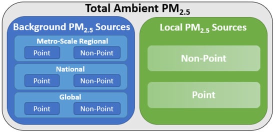
Figure 1.
Total ambient PM2.5 source attribution. Background is defined for the purpose of this paper as the baseline ambient PM2.5 not attributable to local sources (i.e., transported PM2.5 from global (across country lines), national (across state lines), or metro-scale regional (across city/town boundaries, e.g., Dallas, Arlington, or Fort Worth) sources combined). Total ambient PM2.5 can be from natural or anthropogenic sources and includes primary and secondary PM2.5, which can occur at various spatial scales (local, regional, national, and global).
The Dallas–Fort Worth, TX, area has received an abundance of news coverage and scientific interest recently due to its reported decline in air quality and the potential negative health impacts from air pollution [6,7,8,9,10]. The Dallas–Fort Worth area was ranked as the 16th most polluted city for ozone (previously ranked 17th) and 44th worst for short-term particle pollution [6]. Both ozone and PM are attributable to point and non-point sources such as power plants, industrial boilers, and vehicles [9,11]. In the Dallas–Fort Worth area there has been particular interest in industrial sources [12] and the high volume of traffic [13]; the Dallas area has approximately 11,500 miles of traffic lanes, with vehicles logging nearly 77.5 million miles each day [9]. Additionally, the city of Dallas has recently committed to implementing more air monitors to help with tracking neighborhood-level air quality [7].
A review of literature published on PM2.5 in the Dallas–Fort Worth area revealed there are studies that investigated the spatial variability in PM2.5 [14] and the temporal variability in PM2.5 (specifically during the COVID-19 pandemic) [15]. Dallas–Fort Worth area research has also focused on potential methods to estimate PM2.5 levels in areas without monitor data and at finer temporal intervals using Dallas as a case study [16,17], the potential contribution from biomass burning to ambient PM in Dallas and San Augustine, TX [18], and the potential contribution from the transportation sector to PM2.5 in Dallas [13]. Source apportionment has been investigated in other Texas cities including Corpus Christi [19] and Houston [4]. To our knowledge, only one study has attempted to apportion local vs. regional PM2.5 emissions in the Dallas area, and further apportion the local and regional PM2.5 contributions from point, mobile, and area sources [20]. However, this study relied on monitoring data from 1999 to 2003, utilized a different modelling methodology (i.e., response-surface model representation of the Community Multiscale Air Quality model) to predict future PM2.5 changes for nine urban areas in the United States, and is unpublished, although available online.
Thus, no recently published studies focus on apportioning the local vs. background PM2.5 sources in the Dallas–Fort Worth area, and none have utilized the combination of methods presented herein. We present an approach that combines interpolation and fixed effect regression models to disentangle background from local PM2.5 contributions to the total ambient PM2.5 observed. We provide preliminary insights into the contribution from local point and non-point sources (e.g., vehicle and railroad transport) to the Dallas–Fort Worth area. This methodology demonstrates a new data-driven approach that is more comprehensive than what has previously been demonstrated for the Dallas–Fort Worth area. Finally, this approach can be useful in optimizing potential mitigatory, regulatory, and/or community efforts to reduce ambient PM2.5 concentrations towards the appropriate spatial scale (i.e., local, regional, or state) and sectoral emissions sources (i.e., residential, industrial, transport, etc.).
The most common methods of PM2.5 source contribution apportionment (spatially and by sector) utilized in other metropolitan areas include (1) air sample collection upwind and downwind of suspected sources, (2) modeling air quality impacts based on emission information from various sources, (3) a combination of data collection and modeling, or (4) statistical or chemical analysis of air pollution measurements. Source apportionment methods have various names for the different approaches that utilize monitoring and/or modeling, including “potential impact” or the “Brute Force Method” [21,22], the “incremental approach” [21,23], and “tagging” [21,24]. Additionally, monitoring (i.e., observed concentrations) can include measuring overall PM2.5 air concentrations or evaluating the particulate matter chemical composition, where the major chemical components of PM are measured individually (e.g., ammonium, elemental carbon, organic carbon, sodium, nitrate, potassium, and sulfate) [2]. Because of the spectrum of issues associated with site complexity, data quality, and data representativeness, application of these methods and approaches have varying degrees of success, and range in their strengths and weaknesses, accessibility, and practicality [25]. The data-driven methodology that we use and explain in this article provides an additional approach that is comprehensive, accurate, and reliable, and can be easily applied to any unique location where observational data are abundant.
The “incremental approach”, referenced above, is one of the most popular approaches to source apportionment. The incremental approach compares a background site to the site of interest (commonly a city); many researchers have utilized the incremental approach to estimate the influence of background and/or transported PM2.5 [26,27,28]. For example, Pitiranggon et al. (2021) utilized data from the USEPA Chemical Speciation Network (CSN) and the New York City Community Air Survey (NYCCAS) to compare a background site with 60 sites within New York City (NYC); the comparison was used to examine temporal changes in local and regional (i.e., background) contributions to PM2.5 levels within the city [26]. The authors concluded that regional transport of PM2.5 accounted for 25–46% of total PM2.5 measured in NYC in 2018, a decrease from 2002 when the estimate for regional PM2.5 transport attribution was 46–57%.
Alternatively, observational data and modelling can be presented together as multiple lines of evidence for spatial source apportionment. For example, in the Houston area, Allen and Turner (2008) utilized observational data from Federal Reference Method (FRM) sampling sites, HYSPLIT modeling, and particle composition to determine the influence of regional transport on urban PM concentrations [4]. The authors presented the spatial homogeneity of the PM concentrations as an indicator of the extent of local point source strength; localized point sources tend to introduce spatial gradients in observed PM concentrations. The data presented suggest that both regional and localized PM emission events occur at roughly the same frequency in the Houston area. The HYSPLIT model indicated that high levels of “background” or regional PM2.5 are transported from the eastern part of the United States into the Texas Gulf Coast. Finally, particle composition allowed the authors to conclude that there was seasonal and spatial homogeneity across the Houston sites (i.e., bulk composition was generally similar between sites located in different settings and at a distance from each other).
In addition to spatial apportionment, PM2.5 emissions can be apportioned by sector. For example, Thunis et al. (2018) attempted to quantify the origins of air pollution from a sectoral perspective (transport, residential, agricultural, natural, etc.), and spatial perspective (urban, regional, or country level), by using the “Screening for High Emission Reduction Potentials for Air quality” tool (SHERPA) [5] (the SHERPA tool utilizes source-receptor relationships (SRR), which are simplified chemistry transport models (CTMs) that simulate the contribution to concentration levels due to precursor emissions from one particular area using an emissions inventory). The authors report that a city core’s PM2.5 contribution (i.e., local contribution) to the overall annual PM2.5 concentration is, on average (across the 84 cities included), around 26%, with the highest contribution in Milan at 57%. Additionally, the percentage contribution by sector was found to be city-specific, even for cities located in the same European country. Paris, Madrid, Berlin, and London showed a large impact from the transport sector, while cities in Poland, the Baltic area, and Italy were dominated by residential impacts. Sector source apportionment has also been conducted in the United States using USEPA CSN; vehicle traffic has been suggested to be the largest source of PM2.5 in the United States [29].
Statistical methods may also be used to isolate background influence from local PM2.5 influence, but these methods tend to only evaluate specific areas or specific background sources, and their results cannot necessarily be translated to other areas [30,31,32]. In these studies, researchers use regression models to relate total concentrations at a given location to background concentrations at other locations.
The methods discussed above have clear limitations and can introduce uncertainties into the results that impact accuracy, interpretability, spatiotemporal resolution, and/or generalizability. Monitoring can be highly dependent on the location, quality of the monitors, and the frequency and composition of the data from the monitors; however, when monitoring data are robust, as in our analysis, approaches that utilize observational data are more reliable and accurate compared to modeling methodologies that may not represent reality. Models are highly dependent on and limited by the true representativeness of their inputs, and many have high computational costs. Independent of the method or combination of methods utilized, the literature clearly demonstrates that local, regional, national, and even global PM2.5 sources each contribute to the observed PM2.5 levels; however, the split among these factors varies greatly over time and/or location.
People spend about 70% of their time in their homes [33] and can be exposed to high levels of PM2.5 while indoors (about 40% of the PM2.5 is from indoor sources and 60% of the PM2.5 is external PM2.5 that has infiltrated the home) [34]. Despite the large portion of an individual’s PM2.5 exposure being from indoor sources, the identification, monitoring, and reduction of national, regional, and local sources of ambient, external PM2.5 has been the primary focus of legislation in the United States since the late 1990s, as governed by the Clean Air Act (CAA) [35,36]. Again, such efforts require the ability to identify the portion of PM2.5 that is attributable to background or local sources and point or non-point sources to direct targeted, efficient mitigatory and regulatory measures that can help reduce the risk of adverse health outcomes potentially associated with elevated PM2.5 concentrations.
Despite a continual decrease in national ambient PM2.5 levels in the United States since 2000 (a 42% decrease across 361 monitoring sites) [37], general average trends cannot accurately represent local PM2.5 levels experienced throughout the country. Additionally, while the United States is considered to have overall “good” air quality compared to other countries, there can be local, temporal, or spatial increases in PM2.5 concentrations, potentially exceeding the current health-based National Ambient Air Quality Standards (NAAQS) for PM2.5 (the current NAAQS are 12 µg/m3 for primary annual average ambient levels, 15 µg/m3 for secondary annual average ambient levels, and 35 µg/m3 for 98th percentile 24-h primary and secondary ambient levels [16]; however, on 6 January 2023, the USEPA announced its proposed decision to revise the primary (health-based) annual PM2.5 standard from its current level of 12 µg/m3 to within the range of 9.0 to 10.0 µg/m3 [38]).
We focused on the Dallas–Fort Worth metropolitan area as a case study because of the increased attention on air quality, the U.S. Environmental Protection Agency’s (USEPA) data availability, the mixture of multiple natural and anthropogenic PM2.5 sources, and the relatively flat and consistent elevation in the area. Despite being currently in attainment of the PM2.5 NAAQS, the Dallas core-based statistical area (CBSA) is the fourth most populated CBSA in the United States [39] and includes a variety of PM2.5 sources. PM2.5 in Dallas is characterized by peaks in the summer and lows in the late fall and winter [40]. Although many areas of the United States experience PM2.5 peaks in the winter, other areas experience peaks in the summer because of meteorology and vehicle traffic [40]. Understanding the most significant contributing sources to observed PM2.5 exposure levels in this region can help identify the key contributing sources that could result in the most significant potential reductions in PM2.5 exposure. Thus, while this article evaluates the Dallas–Fort Worth area, utilizing publicly available monitoring data and accessible methodology, the intent is that this approach simplifies this type of evaluation so that it may be replicated and utilized by researchers at other locations in the future.
2. Materials and Methods
2.1. Data Download and Data Processing
We downloaded all available 24-h PM2.5 data for the state of Texas from the USEPA’s Outdoor Air Quality Data download page for 2013 to 2022 [41]. In some cases, a given monitor location had multiple data points for a given day. These multiple data points were resolved as follows. Within the USEPA Outdoor Air Quality Data, the Parameter Occurrence Code (POC) identifies the number of devices measuring the same pollutant at a monitoring location [42]. Therefore, in cases where the POC was greater than 1, data points for a given day were averaged. The USEPA Outdoor Air Quality Data also flags data from monitors of varying quality. Data with the Air Quality System (AQS) Parameter “PM2.5—Local Conditions” are from Federal Reference Methods (FRM), Federal Equivalent Methods (FEM), or other methods that are to be used in making NAAQS decisions. Data with the AQS Parameter “Acceptable PM2.5 AQI & Speciation Mass” are valid data that reasonably match the FRM but cannot be used in NAAQS decisions. For days in which there were data with both the AQS Parameter “PM2.5—Local Conditions” and “Acceptable PM2.5 AQI & Speciation Mass”, the data with AQS Parameter “PM2.5—Local Conditions” were selected, as this code represents the highest quality data [43]. We subset the dataset to focus on the monitoring locations within the Dallas CBSA (n = 11). We then log-transformed the data because it appeared to follow a log-normal distribution.
We also mapped the location of each monitoring location and calculated the distance between each monitoring location and the nearest roadway and rail line. Total PM2.5 measured at a monitoring location is a combination of local sources and background influence. Background PM2.5 represents short- and long-range transported PM2.5 from global-, national-, or metro-scale regional sources combined. Local PM2.5 is defined as PM2.5 not observed at other within-CBSA monitors and is inherently defined by the available monitoring network included in the analysis. The minimum distance between Dallas CBSA PM2.5 monitors is 5 km, and the median distance between a Dallas CBSA PM2.5 monitor and its nearest neighboring monitor is 10 km. The definition of “local” for this analysis can, therefore, be thought of as a radius of a few km to about 5 km surrounding a given monitor.
2.2. Total PM2.5 Descriptive Statistics
For each monitoring location in the Dallas CBSA, we calculated total PM2.5 summary statistics to characterize within- and between-monitor variability. For each monitoring location, we also calculated an intra-cluster correlation (ICC) coefficient at the month–year level to aid in regression modeling specification. The ICC is a measure of the similarity between measurements within a month–year, with a value of zero representing no similarity, and a value of 1 representing homogenous measurements within a month–year. If the ICC was statistically greater than zero, the measurements within a month–year were said to be clustered and were not independent. Subsequent regression models then needed to account for that clustering to appropriately characterize model precision (i.e., to appropriately calculate model output standard errors.
Because we evaluated data across a 10-year period, we identified the clusters as “month–year” to clarify that each month in each year, rather than each month across all years, is its own cluster (e.g., September 2013 and September 2014 are distinct clusters, and there is no September cluster).
2.3. Fixed Effects Model Controlling for Temporal Variability
To further characterize between-monitor variability, we built a fixed effects model using the log-transformed total PM2.5 data that controlled for annual and monthly variability. Due to differences in year-to-year and month-to-month data availability for each monitoring location, it is uncertain if any potential differences in mean total PM2.5 concentrations observed in the descriptive statistics (Section 2.2) are due to actual concentration differences by location or differences in data availability. The model also accounted for clustering at the month–year level. Equation (1) describes the fixed effect model, which is based in part on the model developed by Karppinen et al. (2004) [30]:
where PMijym is the total PM2.5 concentration for day i in year y and month m at location j, locationj is an indicator variable for the monitoring location, βj represents the coefficients for the location indicator variable, δy are the fixed effects for each year, δm are the fixed effects for each month, and εijym is the model residual. The fixed effects model is most appropriate because it assumes that there are unmeasured factors that influence total PM2.5 concentrations that are associated with each year and month. We used this model to calculate 2022-adjusted average total PM2.5 concentrations for each location for each month. Note that our calculation of the average PM2.5 concentrations differs from the calculation of the NAAQS summary statistics [44] and is, therefore, not applicable for comparison with NAAQS standards.
ln(PMijym) = βjlocationj + δy + δm + εijym,
All fixed effects models were developed in the R software program using the “felm” (i.e., fixed effects linear model) function in the “lfe” package. Fixed effects models, like simple linear regression models, use ordinary least squares modeling to estimate both the model coefficients and fixed effects.
2.4. Pairwise Correlation Matrices
To further characterize between-monitor total PM2.5 variability, we calculated Spearman correlation coefficients for each Dallas CBSA monitoring location with each of the other Dallas CBSA monitoring locations. Each pairwise correlation coefficient was populated into a correlation matrix. We also calculated the distance between each of the monitors and plotted these distances with each pairwise correlation coefficient.
2.5. Inverse Distance Weighted Background Average Correlations
The correlations described in Section 2.4 can be used to describe the relationship between total PM2.5 concentrations at one monitor and total PM2.5 concentrations at another monitor. However, they do not account for the relationship between total PM2.5 concentrations at one monitor and all other nearby monitors. Multivariate regression could theoretically be used to evaluate the relationship between one monitor and all other nearby monitors, adjusting for each individual monitor’s relationship, if data are available for all monitors for many days. However, in our dataset, each monitoring location only had data available approximately every three days, thus, not satisfying the requirements of multivariate regression.
Therefore, for each day and for each Dallas CBSA monitoring location, we calculated the background PM2.5 concentration as the inverse distance weighted (IDW) average of total PM2.5 concentrations from all other Dallas CBSA monitoring locations with data for that day (i.e., up to ten monitoring locations (N − 1)). In other words, for each day, each monitoring location had its own corresponding background average. Inverse distance weighted average background PM2.5 concentrations were calculated using the following equation:
where PMBij is the 24-h background total PM2.5 concentration for monitor j on date i, PMiz is the 24-h total PM2.5 concentration for monitor z on date i, djz is the distance between monitor j and monitor z, and ni is the number of monitors in the Dallas CBSA with valid data on date i.
2.6. Inverse Distance Weighted Background Average Multivariate Regressions
In addition to background air quality, there are other factors that can influence total PM2.5 concentrations at a given location on a given day. In Section 2.3, we hypothesized that each year and month might have a unique effect. Weather may also affect total PM2.5 concentrations. Therefore, weather data from Red Bird Airport in Dallas were downloaded from the Iowa Environmental Mesonet [45]. Additionally, we hypothesized that each location might have a unique relationship between its total PM2.5 concentrations and the background concentration. Therefore, we added to the model from Section 2.3 and produced a fixed effect model that estimates total PM2.5 as a function of background PM2.5, location, temporal variables, and weather variables. The model clustered standard errors at the month–year level. The following equation describes the model:
where PMijymd is the total PM2.5 concentration for day i in year y and month m at location j on day of the week d; locationj is an indicator variable for monitoring location; βj represents the coefficients for the location indicator variable; PMBij is the IDW estimate of background 24-h PM2.5 for day i and location j; β1 is the coefficient for PMBij; locationj × PMBij is the interaction term between location and background PM2.5, allowing each location to have a unique relationship with background PM2.5; β2,j are the coefficients for the location-background PM2.5 interactions; Ti is the demeaned average temperature in Fahrenheit for day I; β3 is the coefficient for the temperature variable; Hi is the demeaned average relative humidity (%) for day i; β4 is the coefficient for the relative humidity variable; Wi is the demeaned average wind speed in knots per hour for day i; β5 is the coefficient for the wind speed variable; Pi is the demeaned average atmospheric pressure in millibars for day i; β6 is the coefficient for the atmospheric pressure variable; δy are the fixed effects for each year; δm are the fixed effects for each month; δd are the fixed effects for each day of the week; and εijymd is the model residual.
ln(PMijymd) = βjlocationj + β1PMBij + β2,jlocationj × PMBij +β3Ti + β4Hi + β5Wi +
β6Pi + δy+ δm + δd + εijymd,
β6Pi + δy+ δm + δd + εijymd,
We ran 12 versions of this model, each with month-specific demeaned weather variables and the month of interest as a referent group and the referent location equal to zero (i.e., no location) so that the coefficients for the location indicator variable can be interpreted as the natural logarithm of the mean total PM2.5 concentration at average weather conditions, zero background PM2.5, and at reference conditions (the month of interest in 2022 on a Tuesday) (additional preliminary analyses identified Tuesdays to have average concentrations most like the overall averages).
Finally, location- and month-specific local attribution were derived by dividing the local contribution by the 2022-adjusted mean total PM2.5 estimates.
In this fixed effect model, we considered the possibility that the background effect coefficients (i.e., β1 and β2,j) and the local contribution effect coefficients (i.e., βj) could be biased due to omitted variable bias (i.e., confounding variables). Namely, unmeasured variables that are associated with both background PM2.5 concentrations and total PM2.5 concentrations that could bias these coefficients. We hypothesized that time-dependent PM2.5 -generating activity that does not transport emissions regionally would be positively correlated with both total concentrations and background concentrations. Essentially, in our regression, some amount of total PM2.5 contributions (i.e., βj) could be incorrectly captured in the background effects (i.e., β1 and β2,j), rather than in the local effects (i.e., βj). This activity could, therefore, bias the background effects upwards and the local effects downwards. To assess the potential for such omitted variable bias, we conducted the following sensitivity analysis.
2.7. Sensitivity Analysis: Texas Correlations
We developed the same correlation matrices as in Section 2.4 but for all EPA PM2.5 monitors in Texas, and plotted the results. This sensitivity analysis allows us to observe if the within-Dallas total PM2.5 correlations are due to common PM2.5-generating activity patterns or common background PM2.5 sources. In other words, any PM2.5 correlations could be due to PM2.5-producing activities that vary by day and are common to all urban areas and not common PM2.5 sources.
We compared Dallas total PM2.5 concentrations with total PM2.5 concentrations in El Paso. We selected El Paso as a comparison region because it is the urban area in Texas with available PM2.5 data that is farthest from Dallas. Of all urban areas in Texas, El Paso likely shares the least background PM2.5 with Dallas; however, as an urban area, El Paso likely shares some common human activity (i.e., PM2.5-generating activity) patterns with Dallas.
3. Results
3.1. Data Download and Data Processing
From 2013 to 2022, there were 71 unique monitoring locations in Texas, and 11 of those were located in the Dallas CBSA. Table 1 shows the distance between each Dallas CBSA monitoring location and the nearest major roadway and rail line.

Table 1.
Distance (meters) between monitoring locations and nearest roadways and rail lines.
Figure 2 presents the locations of the 11 monitors analyzed within the Dallas CBSA; the maximum distance between the monitors contained within the Dallas CBSA was 120 km, while the closest monitors were about 5 km apart.
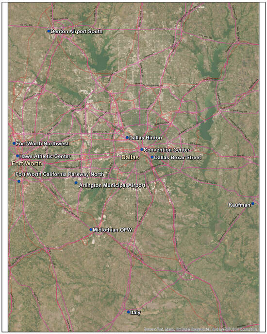
Figure 2.
Location of Dallas–Fort Worth CBSA USEPA monitors (n = 11) shown at dots. Major roadways and railways are shown as lines with railways shown as hatched lined.
3.2. Total PM2.5 Descriptive Statistics
Table 2 shows the raw summary statistics for each Dallas CBSA monitoring location. Additionally, we have included the temporal extent of each monitoring location’s data. In terms of between-monitor variability, the raw mean 24-h total PM2.5 ranged from 7.5 µg/m3 (Kaufman) to 9.6 µg/m3 (Convention Center; Dallas Bexar Street). Note that while there are small differences in the calculated means and medians, the overall ranges of observed 25th to 75th percentiles from each of these locations are nearly indistinguishable; the interquartile ranges (IQRs) ranged from 4.3 µg/m3 (Midlothian OFW) to 5.4 µg/m3 (Dallas Hinton).
Table 2.
Raw Dallas CBSA 24-h total PM2.5 summary statistics (µg/m3).
Within each month–year, depending on the location, the ICC was 0.15 to 0.26 and statistically greater than zero, suggesting that the observations within each month–year are not independent, and that calculation of standard errors should involve clustering.
3.3. Fixed Effects Model Controlling for Temporal Variability
Demonstrating the clustering effect at the month–year level provided justification for building the model parameterized in Equation (1). Exponentiating the coefficients from that model allowed us to calculate 2022-adjusted mean total PM2.5 concentrations for each monitoring location and each month, as seen in Figure 3 and Table S1. In January, the month with the lowest mean concentrations, the mean 24-h total PM2.5 concentration ranged from 5.0 µg/m3 (Kaufman) to 6.4 µg/m3 (Convention Center; Dallas Bexar Street). The 95% confidence limits span from about 1.0 µg/m3 (Denton Airport South; Italy; Kaufman) to 1.9 µg/m3 (Dallas Bexar Street). In July, the month with the highest mean concentrations, the mean 24-h total PM2.5 concentration ranged from 8.7 µg/m3 (Kaufman) to 11.1 µg/m3 (Convention Center; Dallas Bexar Street). The 95% confidence limits spanned from about 2.1 µg/m3 (Denton Airport South; Kaufman) to 3.6 µg/m3 (Dallas Bexar Street). March and April had the median mean concentrations (i.e., average concentrations most similar to the annual average). During March, mean total concentrations ranged from 5.7 µg/m3 (Kaufman) to 7.2 µg/m3 (Convention Center; Dallas Bexar Street). During April, mean total concentrations ranged from 6.0 µg/m3 (Kaufman) to 7.6 µg/m3 (Convention Center; Dallas Bexar Street).
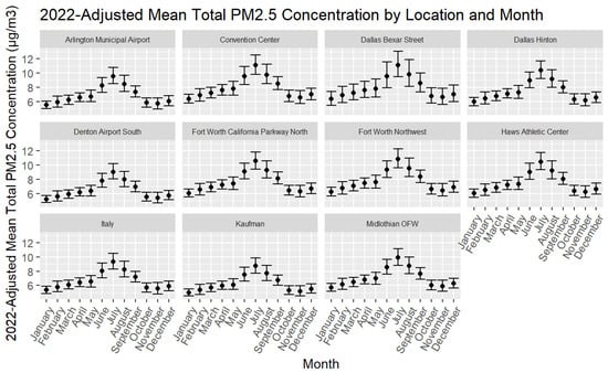
Figure 3.
The 2022-adjusted mean total PM2.5 concentration by location and month. Numerical estimates are included as Table S1.
3.4. Pairwise Correlation Matrices
Within the Dallas CBSA, we developed pairwise 24-h total PM2.5 concentration correlation matrices. Table S2 shows the Spearman correlations. Spearman correlations ranged from 0.73 to 0.92. Figure 4 shows how the Spearman correlations vary by distance.
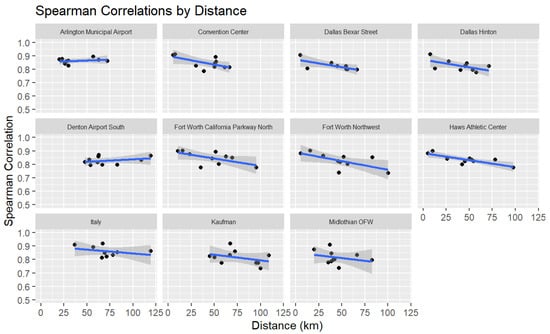
Figure 4.
Pairwise Spearman correlations by distance. Values are correlations between Dallas CBSA 24-h PM2.5 concentrations.
3.5. Inverse Distance Weighted Background Average Correlations
For each monitoring location and each day that the monitoring location had data, we calculated the corresponding background (i.e., from surrounding monitors in the Dallas CBSA from 5 to 120 km away) IDW average PM2.5 24-h concentration; summary statistics for the background data are included as Table S3. These data are not adjusted for temporal variables but are directly comparable with the total concentration data presented in Table 2. We have also included the mean difference between the total and background weighted average. A positive value indicates that the background weighted average is greater than the total concentration, and a negative value indicates that the total concentration is greater than the background weighted average. The mean difference between the total and corresponding background data ranged from −0.7 µg/m3 to 1.1 µg/m3.
Each monitoring location’s measured total concentration dataset was highly correlated with its calculated IDW average background concentration dataset, as seen in Table 3. Spearman correlations ranged from 0.86 to 0.94.
Table 3.
Correlation between each monitoring location’s measured total 24-h PM2.5 concentration and its calculated IDW average background 24-h PM2.5 concentration.
3.6. Inverse Distance Weighted Background Average Multivariate Regressions
Because total and background PM2.5 are highly correlated, we built fixed effect models that regressed total concentration on the monitoring location, while adjusting for background concentrations and other potential confounders. These regressions allowed us to estimate mean total concentrations at each location that are independent of background concentrations (i.e., local contributions). We also allowed each monitoring location to have a unique relationship with its background concentrations by including an interaction effect in the model. Based on the outputs of these fixed effects models, we constructed Figure 5, Table 4 and Table S4.
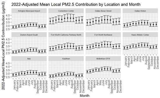
Figure 5.
The 2022-adjusted mean local PM2.5 contributions by location and month. Adjusted for year, month, day of the week, temperature, relative humidity, atmospheric pressure, wind speed, and background PM2.5.
Table 4.
The adjusted 1 effect of background PM2.5 concentration on total PM2.5 concentration by location.
As seen in Figure 5 and corresponding Table S4, in January, the month with the lowest mean local contributions, the local PM2.5 contributions ranged from 2.6 µg/m3 (Denton Airport South; Kaufman) to 3.6 µg/m3 (Convention Center). The 95% confidence limits spanned from about 0.4 µg/m3 (several locations) to 0.9 µg/m3 (Dallas Bexar Street). In July, the month with the highest local PM2.5 contributions, the local PM2.5 contributions ranged from 2.9 µg/m3 (Kaufman) to 4.1 µg/m3 (Convention Center). The 95% confidence limits spanned from about 0.6 µg/m3 (several locations) to 1.1 µg/m3 (Dallas Bexar Street; Convention Center). December and May had the median mean local contributions (i.e., average concentrations most similar to the annual average). During December, mean local concentrations ranged from 2.7 µg/m3 (Kaufman) to 3.8 µg/m3 (Convention Center). During May, mean concentrations ranged from 2.8 µg/m3 (Kaufman) to 3.9 µg/m3 (Convention Center; Dallas Bexar Street).
The local attribution percent describes the portion of total PM2.5 that is attributed to local PM2.5 sources. Figure 6 and corresponding Table S5 show the estimated local attribution percent estimates for each monitoring location in each month. As seen in Figure 6, the month with the lowest local attribution was July, in which local attribution ranged from 33% (Denton Airport South; Arlington Municipal Airport; Dallas Hinton; and Fort Worth California Parkway North) to 37% (Midlothian OFW; Convention Center). The months with the highest local attribution were January and November, in which local attribution ranged from 51% (Denton Airport South; Arlington Municipal Airport; Dallas Hinton; and Fort Worth California Parkway North) to 57% (Midlothian OFW; Convention Center).
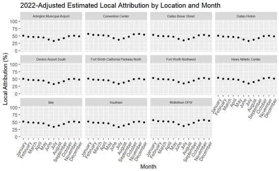
Figure 6.
The 2022-adjusted mean local PM2.5 attribution by location and month.
As seen in Table 4, on average, for each 1 µg/m3 increase in background 24-h PM2.5, the total PM2.5 increased by 9% to 10%.
3.7. Sensitivity Analysis: Texas Correlations
The sensitivity analysis revealed that as the distance between monitors increased, the total PM2.5 concentrations became less correlated. The Dallas CBSA monitoring locations were most correlated with each other, as seen in Figure S1. The Dallas CBSA monitoring locations were not correlated with some monitors in another urban area, El Paso. For example, the Spearman correlation coefficients between the 11 Dallas monitoring locations and the Ascarate Park SE monitoring location in El Paso ranged from 0.0003 to 0.13. Similarly, the Spearman correlation coefficients between the 11 Dallas monitoring locations and the El Paso Chamizal monitoring location in El Paso ranged from 0.01 to 0.15. See Figure 7 for a map of all the Texas monitoring locations.
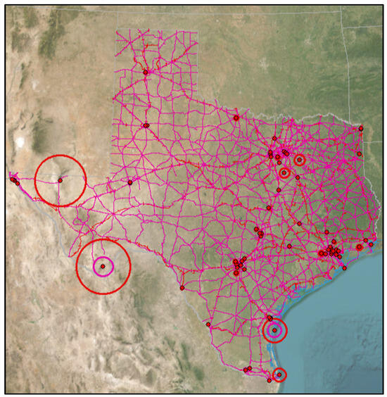
Figure 7.
USEPA monitors (dots), major roadways (lines), and railroads (lines with hash marks); distance to the closest roadway is demonstrated by the pink circle around each monitor, while distance to the closest railroad is represented by the red circle around each monitor.
4. Discussion
In this study, we used fixed effects models and publicly available 24-hour PM2.5 data from the USEPA to calculate average total PM2.5 concentrations in the Dallas–Fort Worth area and the average contribution of background versus local sources near Dallas-area PM2.5 monitors. During March and April, the months with the median mean total concentration, mean total concentrations ranged from 5.7 µg/m3 (Kaufman in March) to 7.6 µg/m3 (Convention Center and Dallas Bexar Street in April) (Figure 3 and Table S1). During the same months, mean local contributions ranged from about 2.7 µg/m3 (Kaufman in March) to 3.9 µg/m3 (Convention Center in April) (Figure 5 and Table S4). Based on comparisons of the mean total PM2.5 concentrations and mean local contributions (Table S5), we conclude that background and local sources each contribute about half of the total PM2.5 at a given location within the Dallas–Fort Worth area.
As described below, the higher PM2.5 concentrations experienced in the summer months appear to be mostly related to background influences and not local contributions —although the specific nature of such seasonal differences has not been identified. Local contributions seem to vary less than total concentrations. For example, at Arlington Municipal Airport, the mean total PM2.5 concentration in July, the month with the highest mean total concentrations, is 74% greater than the mean total PM2.5 concentration in January, the month with the lowest mean total concentrations. Meanwhile, the mean local contribution in July, the month with the highest mean local contributions, is 13% greater than the mean in January, the month with the lowest mean local contributions.
Therefore, the percentage of total PM2.5 attributed to local vs. background sources varies throughout the year. In January, the month with the lowest mean total PM2.5 concentrations, local attribution ranged from 51% to 57%. In July, the month with the highest mean total PM2.5 concentrations, local attribution ranged from 33% to 37%. Thus, the higher concentrations experienced in the summer appear to be mostly attributed to background influences, not local contributions.
While source attribution varies by city and/or area, this finding that, on average, roughly half of the PM2.5 concentration is attributable to local sources falls within the attribution ranges previously reported [5,20,26,27,28]; specifically, a similar finding was reported for Houston, a similarly large, metropolitan area in Texas [4].
Within each month, we found that local (i.e., all non-background sources) contributions only ranged by about ±0.5 µg/m3 across the entire Dallas–Fort Worth area. There was also considerable overlap among the 95% confidence intervals for these total non-background source contribution estimates, suggesting that the range of influence by local point sources is relatively modest. Given that government agencies design their air quality monitoring networks to capture a range of exposures [46], it is possible that the requirements for monitor placement may explain some of the variability both in mean total concentration and mean local contribution.
Apportioning among background and local PM2.5 source contribution is important because accurately identifying potential sources can assist in later evaluating the effectiveness of various mitigation efforts and regulatory approaches. However, it is important to recognize that the local contribution can be further apportioned to differentiate more widely dispersed local non-point sources from geographically-limited local point sources. Common local non-point sources can include exhaust, re-suspension of dust and salt, and brake, tire, and equipment ware from local transport (gasoline and diesel-powered vehicles, railroads, and ships). Local PM2.5 point sources can (depending on the scale) include individual heating sources (residential and commercial), biomass burning, dust from construction, and certain industrial activity and emissions (energy generation, biproducts, disturbance of materials, etc.) [4,5,47].
To investigate the potential impact of non-point sources at our 11 monitoring locations, we conducted a linear regression between the mean local contributions in May in Figure 5 and Table S4 and distances to roadway and rail line in Table 1, as seen in Appendix A. We selected May as the analysis month because we found that median local contributions occurred in May. We found that distance to roadway was inversely correlated with log-concentration with marginal significance, and distance to rail line was inversely correlated with log-concentration with statistical significance; see Figure 7 for location of closest major roadway and rail line. These regressions rely on a small sample size (i.e., 11 monitoring locations), and a more thorough analysis would likely account for traffic or train volume; however, these regressions do suggest that sources such as roadways and trains could explain a significant portion of the variability in mean concentrations and/or mean local contributions.
The results in Dallas are similar to those previously reported for the area, which have identified and reported significant fractions of overall PM2.5 as attributable to local non-point sources (i.e., vehicle traffic) [20]. Similarly, in cities of South Texas, anthropogenic emissions from on-road and off-road traffic from nearby highways were identified as major local contributors [48]. For example, in Houston, the primary non-point sources contributing to overall PM2.5 mass on days not influenced by wood smoke (e.g., wildfires) included diesel-powered vehicles (21%, 22%, and 20%) and gasoline vehicles (17%, 12%, and 9%) [47]. Likewise, our results are similar to results in other cities in the southern part of the United States that rely upon non-public modes of transportation (e.g., Atlanta, GA, USA), where researchers have apportioned a large proportion of observed PM2.5 to traffic-related emissions [4,49,50]. In large European cities (e.g., Paris, Madrid, London), road transport represented up to 39% of overall PM2.5 levels [5]. Previously reported average PM2.5 concentrations of local transport-related emissions range from 0.1 to 2.0 ± 0.2 µg/m3 for major roadways [51], 0.52 ± 0.43 µg/m3 to 1.36 ± 1.30 µg/m3 for oil combustion [28], 1.30 ± 1.26 µg/m3 for highway vehicles [28], and 0.35 ± 0.36 µg/m3 to 2.16 ± 1.32 µg/m3 for diesel [28], depending on the city and/or monitor location (e.g., distance to highway or major roadway). The Dallas–Fort Worth metropolitan area heavily relies on vehicles for transportation; the vast majority of people are reported to drive alone to work, with an average commute time of 28.4 min [52]. Additionally, the average car ownership in Dallas, TX, USA, was two cars per household [52]. Thus, it would make sense for a major portion of the local PM2.5 to be attributable to the transportation sector.
The remaining PM2.5 concentration not explained by background or local non-point source PM2.5 could be attributed to a spectrum of potential local point sources (e.g., individual residential, commercial, or industrial sources) or additional non-point sources (e.g., increased traffic volume, as compared to distance to traffic). However, variability in mean local contribution estimates is limited across the entire Dallas CBSA, despite the variety of monitor locations (i.e., some monitors are located by airports, in residential areas, and in commercially dense downtown areas). Some monitoring locations do have local contribution estimates above the mean local contribution; in such cases, it appears that the remaining local contribution is most likely attributable to concentration variations in the portion of non-point source (e.g., vehicles) emissions that do not transport regionally, rather than significant contributions from individual point sources. This is in agreement with other studies that report small percentages attributable to point sources, as compared to non-point source; for example, in the same Houston study cited above, wood combustion (5%, 5%, and 4%), and meat cooking (8%, 3%, and 6%) were found to be significantly smaller fractions as compared to traffic-related sources [47]. In other words, it appears that the limited variability in, and majority of, local contribution estimates in the Dallas CBSA is due to a ubiquitous source, such as transportation, rather than to a distributed array of point sources that all by chance amount to approximately the same contribution.
To a small extent, we expect the correlations between PM2.5 concentrations at a location and background PM2.5 to be attributable to residual confounding (i.e., bias). In other words, pollution-generating activity (e.g., driving, heating, and industrial patterns) is likely time-dependent. Past research has shown that PM2.5 can travel thousands of kilometers, dependent on conditions [3,4,5]. But even if there were no direct connection between locations, there may still be correlations between monitoring locations’ total PM2.5 concentrations because of common temporal patterns in PM2.5-generating activity. Thus, the background effects shown in Table 4 likely incorporate the influence of both common regional sources and common patterns in PM2.5-generating activity. However, we believe the influence of common PM2.5-generating activity patterns is limited because of our sensitivity analysis. The residual confounding from common PM2.5-generating activity patterns would bias the background effect estimates upward. However, measurement error in inverse distance-weighted background concentration estimates would bias these background effect estimates low. Some amount of measurement error in the background concentration estimates is expected because the true value of the relevant background concentration is unknown. Additionally, our estimates rely only on available monitoring data and do not account for all contributing background area sources. That error could either be unbiased because the Texas Commission on Environmental Quality (TCEQ) monitors a range of conditions, or the background concentration estimates could be biased high because the TCEQ may oversample areas with relatively high concentrations. Regardless, the background concentration estimate error would bias the background effect estimates downward. The combined effect of residual confounding and background concentration measurement error is unknown but is expected to cancel out to some extent.
In our sensitivity analysis relating to the influence of common PM2.5-generating activity, distance, not urbanicity, is the key predictor of correlation between two monitor locations’ PM2.5 concentrations. If common patterns in PM2.5-generating activity (i.e., urbanicity) were the dominant influence in the background effect in Table 4, one would expect faraway urban areas (e.g., Dallas and El Paso) to still be highly correlated. However, we demonstrated that faraway urban areas were correlated in only a limited capacity. Therefore, we believe the background effects in Table 4 could be biased high, if at all—but if so, by an amount unlikely to change the overall conclusions of this study. Similarly, the local contribution estimates may be biased low, but again by an amount unlikely to change the overall conclusions of this study. Furthermore, we expect any biases to be relatively similar for each location. There is no reason to believe that the omitted variable bias would vary by location, especially given the limited variability in local contributions to PM2.5 concentrations, the limited variability in background effects, and the consistently strong correlations between each location’s total concentrations and corresponding background concentrations.
One strength of our analysis is the calculation of temporally-adjusted mean total PM2.5 concentrations using fixed effects models. The available USEPA data ranged in completeness, from newer or incomplete data sets (e.g., the Dallas Bexar Street monitor, which has the shortest operating duration from 2/1/2022–12/4/2022), to more established datasets (e.g., the Dallas monitors that have operated from 1/1/2013–12/31/2022). When comparing PM2.5 datasets with the same temporal extent, a temporal adjustment is likely less important, unless there are large data gaps or a reason to believe there is systematic sampling bias. PM2.5 datasets with different temporal extent should be compared only for screening purposes (e.g., in Table 2), but generally should not be the basis for decision-making. Additionally, by log-transforming our data and clustering standard errors, we can appropriately estimate total PM2.5 central tendencies and our precision in those estimates.
Our analysis also used up to 10 monitors to create a measure of background air pollution for each monitoring location. IDW allowed us to distill data from multiple surrounding monitors into one measurement and circumvent gaps in data overlap. Other methods, such as multiple imputation or machine learning, may have also sufficed to address gaps in data overlap.
While our analysis has good temporal resolution and extent (all available 24-h USEPA data for 10 years), our primary analysis only covers 11 point locations in the Dallas CBSA. These 11 Dallas monitoring locations do not represent the full spatial variability of PM2.5 in Dallas; however, the TCEQ selected these locations to represent a range of conditions, including areas of relatively poor air quality. It is possible that monitoring locations may even oversample such areas [46,53]. Note that our 2022-adjusted mean total PM2.5 concentration estimates are comparable to the EPA’s Office of Air Quality Planning and Standards’ (OAQPS) annual average PM2.5 estimates within the Dallas–Fort Worth metropolitan area (counties considered within the Dallas–Fort Worth Metropolitan Area include Collin, Dallas, Denton, Ellis, Hood, Hunt, Johnson, Kaufman, Parker, Rockwall, Somervell, Tarrant, and Wise) that ranged from 8.57 µg/m3 to 10.0 µg/m3; the OAQPS’ estimates are derived using a fusion of the monitoring data from 2018 and Community Multiscale Air Quality (CMAQ) air quality modeling [51,52].
Another limitation of our study is that we have poor data availability in some cases (e.g., the Dallas Bexar Street monitoring location did not operate until February 2022, and the Arlington Municipal Airport and Italy monitoring locations did not operate through 2022). Therefore, 2022-adjusted values should be interpreted as modeled values, not based solely on measurements, that rely on trends across all Dallas CBSA monitors to provide a best estimate. Nevertheless, this paper provides a methodology for estimating concentrations when data may be limited.
Note that while our analysis utilizes 24-h PM2.5 concentrations, within 24-h periods, PM2.5 concentrations will be both greater and less than the mean 24-h concentrations estimated herein; however, utilizing 24-h PM2.5 concentrations corresponds with the USEPA NAAQS, which are developed specifically with public health in mind [36].
While these findings are specific to the Dallas–Fort Worth area and are appropriate to reference, the specific source apportionment determined here should not be extrapolated to locations outside the area of interest without verification; past studies have indicated high variability in source attribution depending on area and/or city [4,25].
5. Conclusions
The Dallas–Fort Worth area has received increased attention surrounding concerns of poor air quality, specifically for particulate matter and ozone. We have demonstrated that in order to determine the major sources of local PM sources, the background contribution must first be accounted for and understood. Our findings suggest that in order to most efficiently decrease observed PM2.5 across the entire Dallas–Fort Worth geographic area, the primary focus should be on regional (i.e., metro-scale) sources and policies that regulate non-point sources (i.e., transportation).
When evaluating local non-point source or point source contributions to total PM2.5 concentrations, a thorough and reliable analysis is needed. While our results indicate that background PM2.5 sources contribute about half of the observed PM2.5 at an individual location within the Dallas CBSA, we recommend that this technical approach be utilized for any unique location within the Dallas–Fort Worth area as this background influence may vary slightly by the monitor’s surroundings. By utilizing publicly available monitoring data and accessible methodology, we present this approach as a roadmap for evaluating PM2.5 concentrations to optimize any potential mitigatory, regulatory, and/or community efforts to reduce PM2.5 concentrations towards the appropriate spatial scale (i.e., local, regional, or state) and sectoral emissions sources (i.e., residential, industrial, transport, etc.).
Supplementary Materials
The following supporting information can be downloaded at: https://www.mdpi.com/article/10.3390/air1040019/s1, Table S1: 2022-adjusted mean daily total PM2.5 concentration by location and month; Table S2: Spearman correlation matrix of 24-h total PM2.5 concentrations in the Dallas CBSA; Table S3: Raw IDW Average Background Dallas CBSA 24-h PM2.5 summary statistics; Table S4: 2022-adjusted mean 24-h local PM2.5 contributions by location and month; Table S5: Mean local PM2.5 attribution proportions by location and month; Figure S1: Pairwise Spearman correlations between Dallas monitoring locations and other Texas monitoring locations.
Author Contributions
Conceptualization, A.S., S.K. and A.H.L.; methodology, A.S.; software, A.S.; validation, S.K., A.S. and A.H.L.; formal analysis, A.S.; investigation, A.S., S.K. and A.H.L.; resources, S.K. and A.S.; data curation, A.S.; writing—original draft preparation, S.K. and A.S.; writing—review and editing, A.H.L.; visualization, A.S. and S.K.; supervision, A.H.L.; project administration, A.H.L.; funding acquisition, A.H.L. All authors have read and agreed to the published version of the manuscript.
Funding
Roux: Inc. received grant funding from the Asphalt Institute for the preparation and submission of this manuscript.
Institutional Review Board Statement
Not applicable.
Informed Consent Statement
Not applicable.
Data Availability Statement
All PM2.5 data utilized are publicly available at https://www.epa.gov/outdoor-air-quality-data/download-daily-data (accessed on 1 July 2023); weather data is publicly available at https://mesonet.agron.iastate.edu/request/download.phtml?network=TX_ASOS (accessed on 1 July 2023).
Conflicts of Interest
The funders had no role in the design of the study; in the collection, analyses, or interpretation of data; in the writing of the manuscript. Andrew Shapero, Stella Keck, Adam H Love are each employed by the company Roux, Inc. Roux, Inc. is an environmental consulting firm that provides services to clients across the United States. Roux’s services include air quality assessment and source appointment of air quality constituents, including PM2.5. Grant funding for development of this manuscript was obtained through the Asphalt Institute. The authors declare that the research was conducted in the absence of any commercial or financial relationships that could be construed as a potential conflict of interest.
Appendix A. Multivariate Regression Relating Mean Local Effect to Distance to Roadway and Rail Line
We hypothesized that one explanation for the variability in mean local contributions (Figure 5 and Table S4) may be the monitoring locations’ distances from roadways and rail lines. Therefore, we built a multivariate linear regression that related these variables. The form of the regression was as follows:
where βj is the local contribution effect for location j estimated in equation 3 with reference month May, Roadj is the distance between location j and the nearest road, β8 is the coefficient for the road distance variable, Railj is the distance between location j and the nearest rail line, and β9 is the coefficient for the rail distance variable. We selected May as the analysis month because we found that median local contributions occurred in May.
βj = β7 + β8∗Roadj + β9∗Railj,
References
- Anastasopolos, A.T.; Hopke, P.K.; Sofowote, U.M.; Zhang, J.J.Y.; Johnson, M. Local and regional sources of urban ambient PM2.5 exposures in Calgary, Canada. Atmos. Environ. 2022, 290, 119383. [Google Scholar] [CrossRef]
- World Health Organization. Health Effects of Particulate Matter: Policy Implications for Countries in Eastern Europe, Caucasus, and Central Asia; World Health Organization: Geneva, Switzerland, 2021; ISBN 978-92-890-0001-7. [Google Scholar]
- Wang, J.; Zhang, M.; Bai, X.; Tan, H.; Li, S.; Liu, J.; Zhang, R.; Wolters, M.A.; Qin, X.; Zhang, M.; et al. Large-scale transport of PM2.5 in the lower troposphere during winter cold surges in China. Sci. Rep. 2017, 7, 13238. [Google Scholar] [CrossRef] [PubMed]
- Allen, D.T.; Turner, J.R. Transport of Atmospheric Fine Particulate Matter: Part 1—Findings from Recent Field Programs on the Extent of Regional Transport within North America. J. Air Waste Manag. Assoc. 2008, 58, 254–264. [Google Scholar] [CrossRef] [PubMed][Green Version]
- Thunis, P.; Degraeuwe, B.; Pisoni, E.; Trombetti, M.; Peduzzi, E.; Belis, C.A.; Wilson, J.; Clappier, A.; Vignati, E. PM2.5 source allocation in European cities: A SHERPA modelling study. Atmos. Environ. 2018, 187, 93–106. [Google Scholar] [CrossRef]
- Martinez, J.A. New Report: DFW’s Air Quality Gets Worse Residents Exposed to More Unhealthy Air Pollution. American Lung Association. 2022. Available online: https://www.lung.org/media/press-releases/sota-dallas-fy22 (accessed on 1 July 2023).
- Reddy, S. Dallas Tackles Environmental Concerns: 40 Air Monitors by End of 2023. The Dallas Morning News. 2023. Available online: https://www.dallasnews.com/news/2023/03/08/dallas-tackles-environmental-concerns-40-air-monitors-by-end-of-2023/ (accessed on 1 July 2023).
- Khreis, H.; Jack, K.; Johnson, J.; Vallamsundar, S.; Dadashova, B.; Nieuwenhuijsen, M. Breathe Easy Dallas: Measuring the Impact of School-Based Interventions on Air Quality and Daily Asthma Exacerbations at High Risk Schools. Abstract. Environ. Epidemiol. 2019, 3, 197. [Google Scholar] [CrossRef]
- Syed, Z. New Tool Says Dallas-Fort Worth Ranks Third in the World for Transportation-Related Greenhouse-Gas Emissions. KERA News. 2023. Available online: https://www.keranews.org/energy-environment/2023-09-22/new-tool-says-dallas-fort-worth-ranks-third-in-the-world-for-transportation-related-greenhouse-gas-emissions (accessed on 1 July 2023).
- Faheid, D. Air Pollution in Dallas-Fort Worth May Be a Problem. But Is It Unhealthy to Breathe? Fort Worth Star-Telegram. 2023. Available online: https://www.star-telegram.com/news/local/article276122676.html (accessed on 1 July 2023).
- Ground-Level Ozone Basics. EPA. 2023. Available online: https://www.epa.gov/ground-level-ozone-pollution/ground-level-ozone-basics (accessed on 1 July 2023).
- Austin, S. Decades after Closure of Lead Smelter, Voices Rise against Other West Dallas Polluters. The Dallas Morning News. 2021. Available online: https://www.dallasnews.com/news/2021/08/22/decades-after-closure-of-lead-smelter-voices-rise-against-other-west-dallas-polluters/ (accessed on 1 July 2023).
- Askariyeh, M.H.; Venugopal, M.; Khreis, H.; Birt, A.; Zietsman, J. Near-Road Traffic-Related Air Pollution: Resuspended PM2.5 from Highways and Arterials. Int. J. Environ. Res. Public Health 2020, 17, 2851. [Google Scholar] [CrossRef] [PubMed]
- Pinto, J.P.; Lefohn, A.S.; Shadwick, D.S. Spatial Variability of PM2.5 in Urban Areas in the United States. J. Air Waste Manag. Assoc. 2004, 54, 440–449. [Google Scholar] [CrossRef]
- Ghahremanloo, M.; Lops, Y.; Choi, Y.; Jung, J.; Mousavinezhad, S.; Hammond, D. A comprehensive study of the COVID-19 impact on PM2.5 levels over the contiguous United States: A deep learning approach. Atmos. Environ. 2022, 272, 118944. [Google Scholar] [CrossRef]
- Karale, Y.Y. Site-Specific PM2.5 Estimation at Three Urban Scales. Dissertation, University of Texas at Dallas. Available online: https://utd-ir.tdl.org/handle/10735.1/9381 (accessed on 1 July 2023).
- Karale, Y.; Yuan, M. Spatially lagged predictors from a wider area improve PM2.5 estimation at a finer temporal interval—A case study of Dallas-Fort Worth, United States. Front. Remote Sens. 2023, 4, 1041466. [Google Scholar] [CrossRef]
- Jia, Y.; Bhat, S.; Fraser, M.P. Characterization of saccharides and other organic compounds in fine particles and the use of saccharides to track primary biologically derived carbon sources. Atmos. Environ. 2010, 44, 724–732. [Google Scholar] [CrossRef]
- Karnae, S.; John, K. Source apportionment of fine particulate matter measured in an industrialized coastal urban area of South Texas. Atmos. Environ. 2011, 45, 3769–3776. [Google Scholar] [CrossRef]
- Hubbell, B.J.; Phillips, S.B.; Jang, C.; Fox, T.J.; U.S. Environmental Protection Agency, Office of Air Quality Planning and Standards; Research Triangle Park NC, USA. Unpublished work. Relative Contribution of Local vs. Regional Emissions to PM2.5 Concentrations in 9 Urban Areas of the U.S. 2008. [Google Scholar]
- Thunis, P.; Clappier, A.; Tarrason, L.; Cuvelier, C.; Monteiro, A.; Pisoni, E.; Wesseling, J.; Belis, C.A.; Pirovano, G.; Janssen, S.; et al. Source apportionment to support air quality planning: Strengths and weaknesses of existing approaches. Environ. Int. 2019, 130, 104825. [Google Scholar] [CrossRef] [PubMed]
- Huang, Y.; Deng, T.; Zhenning, L.; Wang, N.; Yin, C.; Wang, S.; Fan, S. Numerical simulations for the sources apportionment and control strategies of PM2.5 over Pearl River Delta, China, part I: Inventory and PM2.5 sources apportionment. Sci. Total Environ. 2018, 634, 1631–1644. [Google Scholar] [CrossRef]
- Kiesewetter, G.; Borken-Kleefeld, J.; Schopp, W.; Heyes, C.; Thunis, P.; Bessagnet, B.; Terrenoire, E.; Fagerli, H.; Nyiri, A.; Amann, M. Modelling street level PM10 concentrations across Europe: Source apportionment and possible futures. Atmos. Chem. Phys. 2015, 15, 1539–1553. [Google Scholar] [CrossRef]
- Kranenburg, R.; Segers, A.J.; Hendriks, C.; Schaap, M. Source apportionment using LOTOS-EUROS: Module description and evaluation. Geosci. Model Dev. 2013, 6, 721–733. [Google Scholar] [CrossRef]
- Thunis, P.; Clappier, A.; de Meij, A.; Pisoni, E.; Bessagnet, B.; Tarrason, L. Why is the city’s responsibility for its air pollution often underestimated? A focus on PM2.5. Atmos. Chem. Phys. 2021, 21, 18195–18212. [Google Scholar] [CrossRef]
- Pitiranggon, M.; Johnson, S.; Haney, J.; Eisl, H.; Ito, K. Long-term trends in local and transported PM2.5 pollution in New York City. Atmos. Environ. 2021, 248, 118238. [Google Scholar] [CrossRef]
- Lall, R.; Thurston, G.D. Identifying and quantifying transported vs. Local sources of New York City PM2.5 fine particulate matter air pollution. Atmos. Environ. 2006, 40, S333–S346. [Google Scholar] [CrossRef]
- Qin, Y.; Kim, E.; Hopke, P.K. The concentrations and sources of PM2.5 in metropolitan New York City. Atmos. Environ. 2006, 40, S312–S332. [Google Scholar] [CrossRef]
- Thurston, G.D.; Kazuhiko, I.; Lall, R. A source apportionment of U.S. fine particulate matter air pollution. Atmos. Environ. 2011, 45, 3924–3936. [Google Scholar] [CrossRef]
- Karppinen, A.; Harkonen, J.; Kukkonen, J.; Aarnio, P.; Koskentalo, T. Statistical model for assessing the portion of fine particulate matter transported regionally and long range to urban air. Scand J. Work Environ. Health 2004, 30, 47–53. [Google Scholar] [PubMed]
- Timonen, H.; Wigder, N.; Jaffe, D. Influence of background particulate matter (PM) on urban air quality in the Pacific Northwest. J. Environ. Manag. 2013, 129, 333–340. [Google Scholar] [CrossRef]
- Ahmed, E.; Kim, K.H.; Shon, Z.H.; Song, S.K. Long-term trend of airborne particulate matter in Seoul, Korea from 2004 to 2013. Atmos. Environ. 2015, 101, 125–133. [Google Scholar] [CrossRef]
- EPA. Chapter 16—Activity Factors. In Exposure Factors Handbook; EPA: Washington, DC, USA, 2011. Available online: https://www.epa.gov/sites/default/files/2015-09/documents/efh-chapter16.pdf (accessed on 1 July 2023).
- Bi, J.; Wallace, L.A.; Sarnat, J.A.; Liu, Y. Characterizing outdoor infiltration and indoor contribution of PM2.5 with citizen-based low-cost monitoring data. Environ. Pollut. 2021, 276, 116763. [Google Scholar] [CrossRef] [PubMed]
- EPA. Fact Sheet. Proposed Rule to Implement the Fine Particle National Ambient Air Quality Standards. Available online: https://www3.epa.gov/pmdesignations/1997standards/documents/Sep05/factsheet.htm#:~:text=In%20July%201997%2C%20EPA%20promulgated,5%20concentrations (accessed on 27 December 2022).
- EPA. Federal Register. 40 CFR part 50 [EPA-HQ-OAR-2015-0072; FRL-10018-11-OAR]. In Review of the National Ambient Air Quality Standards for Particulate Matter; EPA: Washington, DC, USA, 2020. [Google Scholar]
- EPA. Particulate Matter (PM2.5) Trends. Available online: https://www.epa.gov/air-trends/particulate-matter-pm25-trends (accessed on 5 July 2023).
- EPA. EPA Proposes to Strengthen Air Quality Standards to Protect the Public from Harmful Effects of Soot. 2023. Available online: https://www.epa.gov/newsreleases/epa-proposes-strengthen-air-quality-standards-protect-public-harmful-effects-soot (accessed on 1 July 2023).
- United States Census Bureau, Population Division. “Annual Estimates of the Resident Population for Counties and County-Equivalents: April 1, 2010 to July 1, 2020” (XLS); 2020 Population Estimates: Washington, DC, USA, 2021.
- Zhao, N.; Liu, Y.; Vanos, J.K.; Cao, G. Day-of-week and seasonal patterns of PM2.5 concentrations over the United States: Time-series analyses using the Prophet procedure. Atmos. Environ. 2018, 192, 116–127. [Google Scholar] [CrossRef]
- EPA. Outdoor Air Quality Data: Download Daily Data. 2022. Available online: https://www.epa.gov/outdoor-air-quality-data/download-daily-data (accessed on 1 July 2023).
- EPA. Outdoor Air Quality Data: What Does the POC Number Refer to? 2022. Available online: https://www.epa.gov/outdoor-air-quality-data/what-does-poc-number-refer#:~:text=POC%20is%20the%20Parameter%20Occurrence%20Code%20and%20is,and%20monitor%20type%20are%20independent%20of%20each%20other (accessed on 1 July 2023).
- EPA. AQS Memos—Technical Note on Reporting PM2.5 Continuous Monitoring and Speciation Data to the Air Quality System (AQS). 2006. Available online: https://www.epa.gov/aqs/aqs-memos-technical-note-reporting-pm25-continuous-monitoring-and-speciation-data-air-quality (accessed on 1 July 2023).
- 40 CFR 50 Appendix N. Available online: https://www.ecfr.gov/current/title-40/chapter-I/subchapter-C/part-50/appendix-Appendix%20N%20to%20Part%2050 (accessed on 1 July 2023).
- Iowa State University. Iowa Environmental Mesonet: Texas ASOS. 2022. Available online: https://mesonet.agron.iastate.edu/request/download.phtml?network=TX_ASOS (accessed on 1 July 2023).
- EPA. Outdoor Air Quality Data, Who Decides Where Monitors Get Placed? 2022. Available online: https://www.epa.gov/outdoor-air-quality-data/who-decides-where-monitors-get-placed (accessed on 1 July 2023).
- Buzcu, B.; Yue, W.; Fraser, M.P.; Nopmongcol, U.; Allen, D.T. Secondary particle formation and evidence of heterogeneous chemistry during a wood smoke episode in Texas. J. Geophys. Res. 2006, 111, D10. [Google Scholar] [CrossRef]
- Karnae, S.; John, K. Source apportionment of PM2.5 measured in South Texas near U.S.A.—Mexico border. Atmos. Pollut. Res. 2019, 10, 1663–1676. [Google Scholar] [CrossRef]
- Ivey, C.E.; Holmes, H.A.; Hu, Y.; Mulholland, J.A.; Russell, A.G. A method for quantifying bias in modeled concentrations and source impacts for secondary particulate matter. Front. Environ. Sci. Eng. 2016, 10, 14. [Google Scholar] [CrossRef]
- Huang, M.; Ivey, C.; Hu, Y.; Holmes, H.A.; Strickland, M.J. Source apportionment of primary and secondary PM2.5: Associations with pediatric respiratory disease emergency department visits in the U.S. State of Georgia. Environ. Int. 2019, 133 Pt A, 105167. [Google Scholar] [CrossRef]
- Mukherjee, A.; McCarthy, M.C.; Brown, S.G.; Huang, S.; Landsberg, K.; Eisinger, D.S. Influence of roadway emissions on near-road PM2.5: Monitoring data analysis and implications. Transp. Res. D Transp. Environ. 2020, 86, 102442. [Google Scholar] [CrossRef]
- North Texas Commission. Demographic Trends in Texas and the DFW Area, Presentation. Texas Demographic Center. 28 July 2022. Available online: https://demographics.texas.gov/Resources/Presentations/OSD/2022/2022_07_28_NorthTexasCommission.pdf (accessed on 1 July 2023).
- EPA. 40 CFR 58 Appendix D. In Network Design Criteria for Ambient Air Quality Monitoring, 1st ed.; EPA: Washington, DC, USA, 2021. [Google Scholar]


Disclaimer/Publisher’s Note: The statements, opinions and data contained in all publications are solely those of the individual author(s) and contributor(s) and not of MDPI and/or the editor(s). MDPI and/or the editor(s) disclaim responsibility for any injury to people or property resulting from any ideas, methods, instructions or products referred to in the content. |
© 2023 by the authors. Licensee MDPI, Basel, Switzerland. This article is an open access article distributed under the terms and conditions of the Creative Commons Attribution (CC BY) license (https://creativecommons.org/licenses/by/4.0/).