
Interpreting the Microwave Spectra of Diatomic Molecules


Abstract
1. Introduction
2. Basic Theory
3. Materials and Methods
4. Results
4.1. Carbon Monoxide (CO)
4.2. Alkali Halides
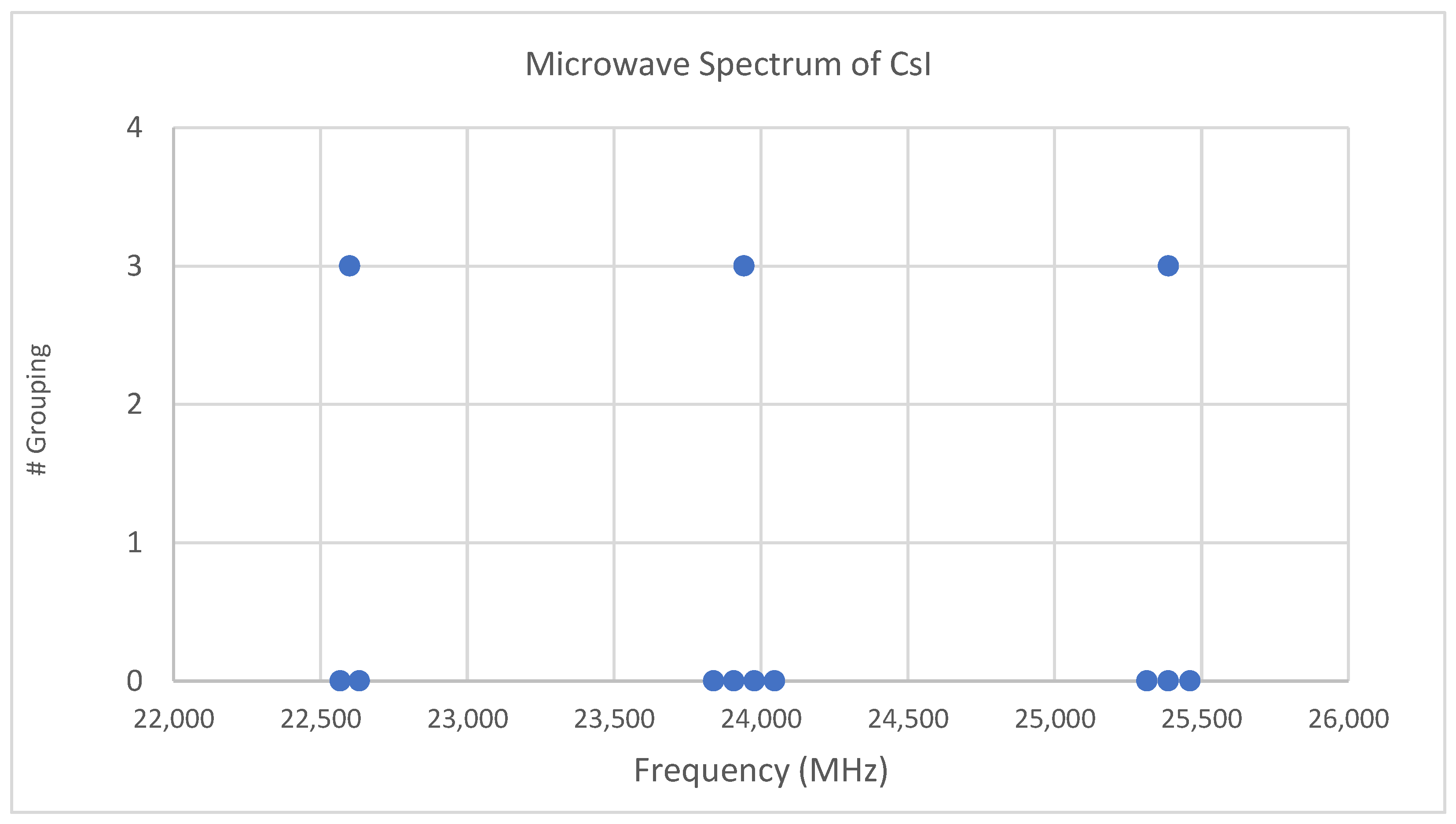
4.3. Cesium Iodide (CsI)
5. Advanced Theory
6. More Results
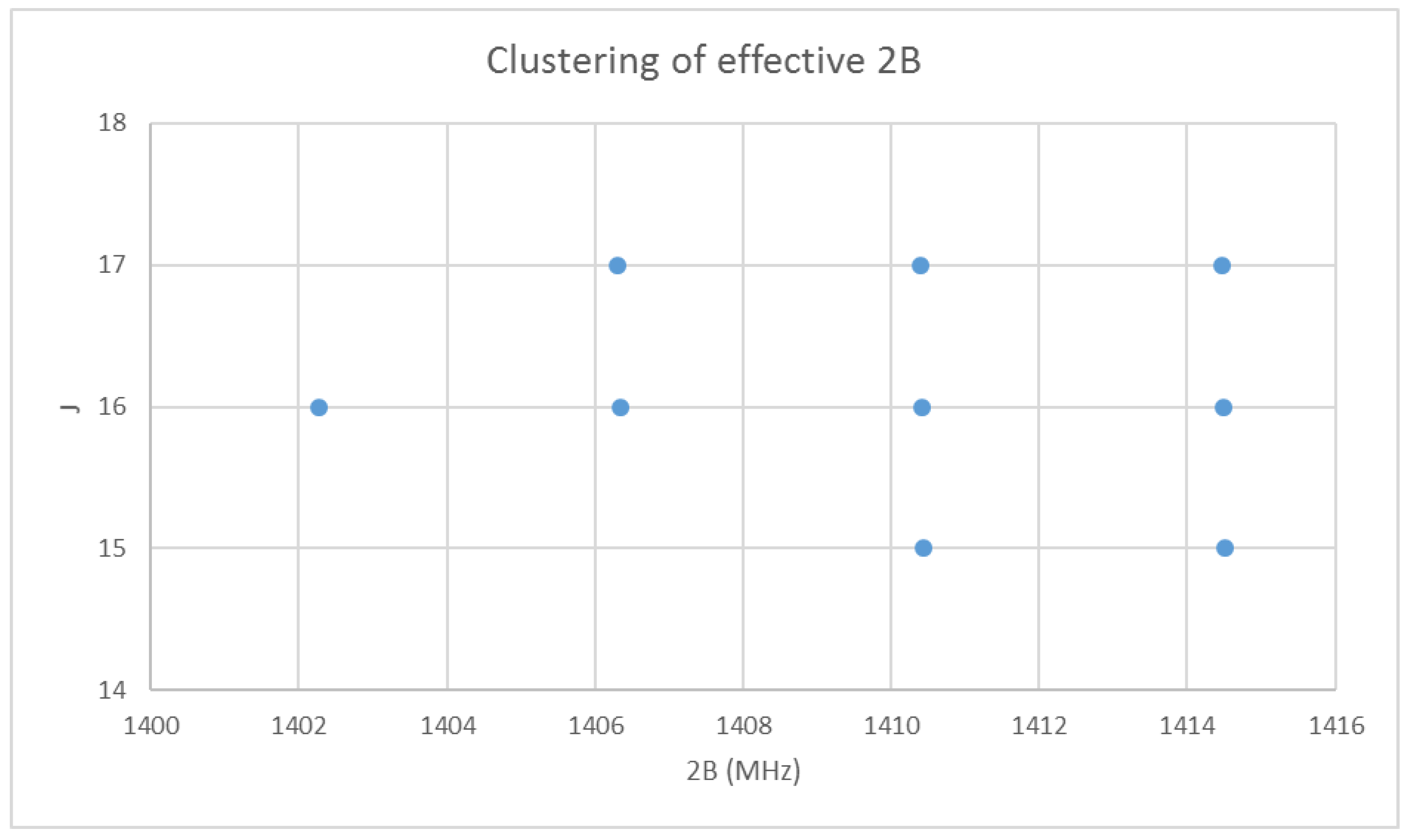
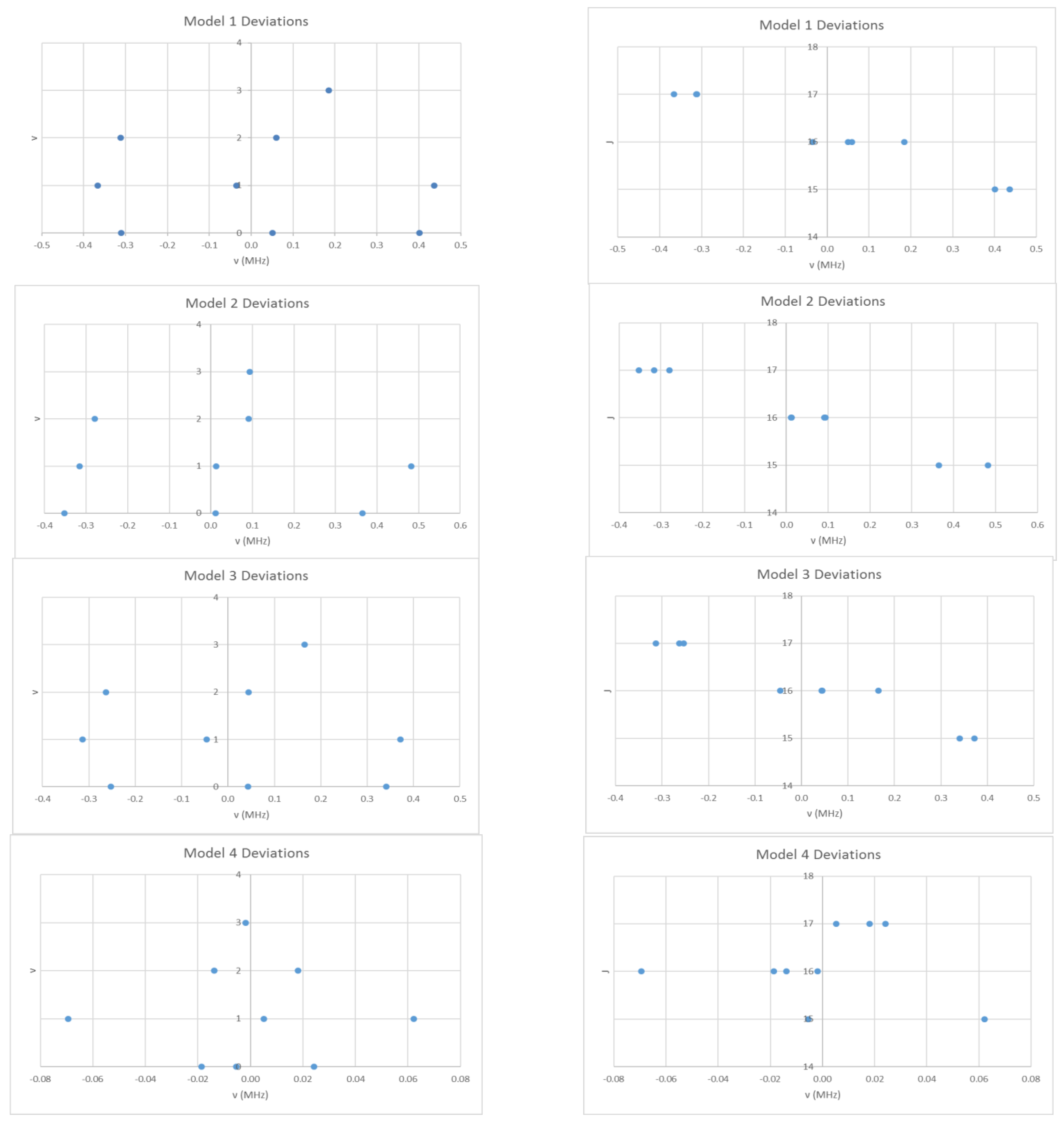
6.1. Cesium Iodide (CsI, Reprise)
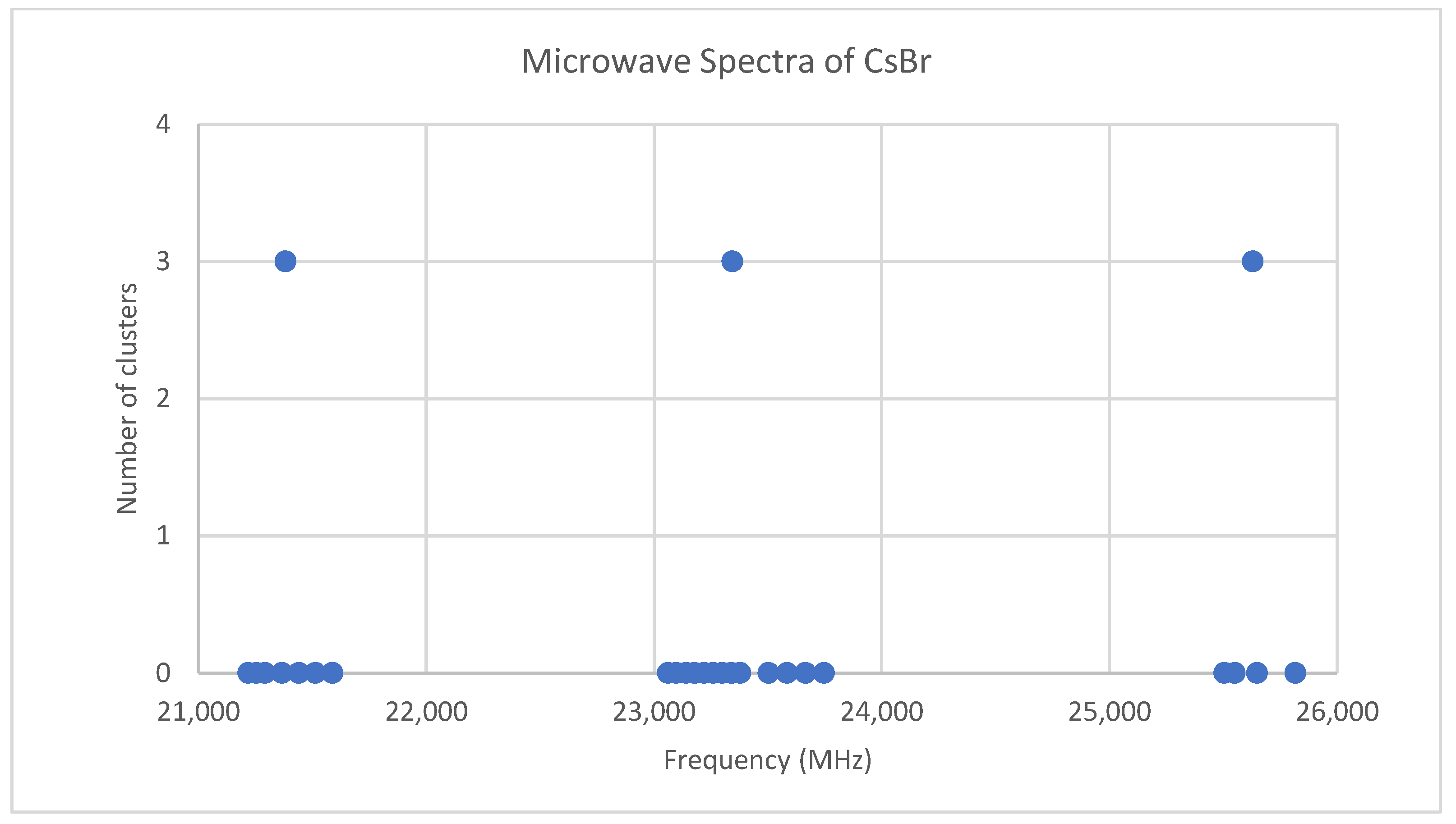
6.2. Cesium Bromide (CsBr)
6.3. Cesium Chloride (CsCl)
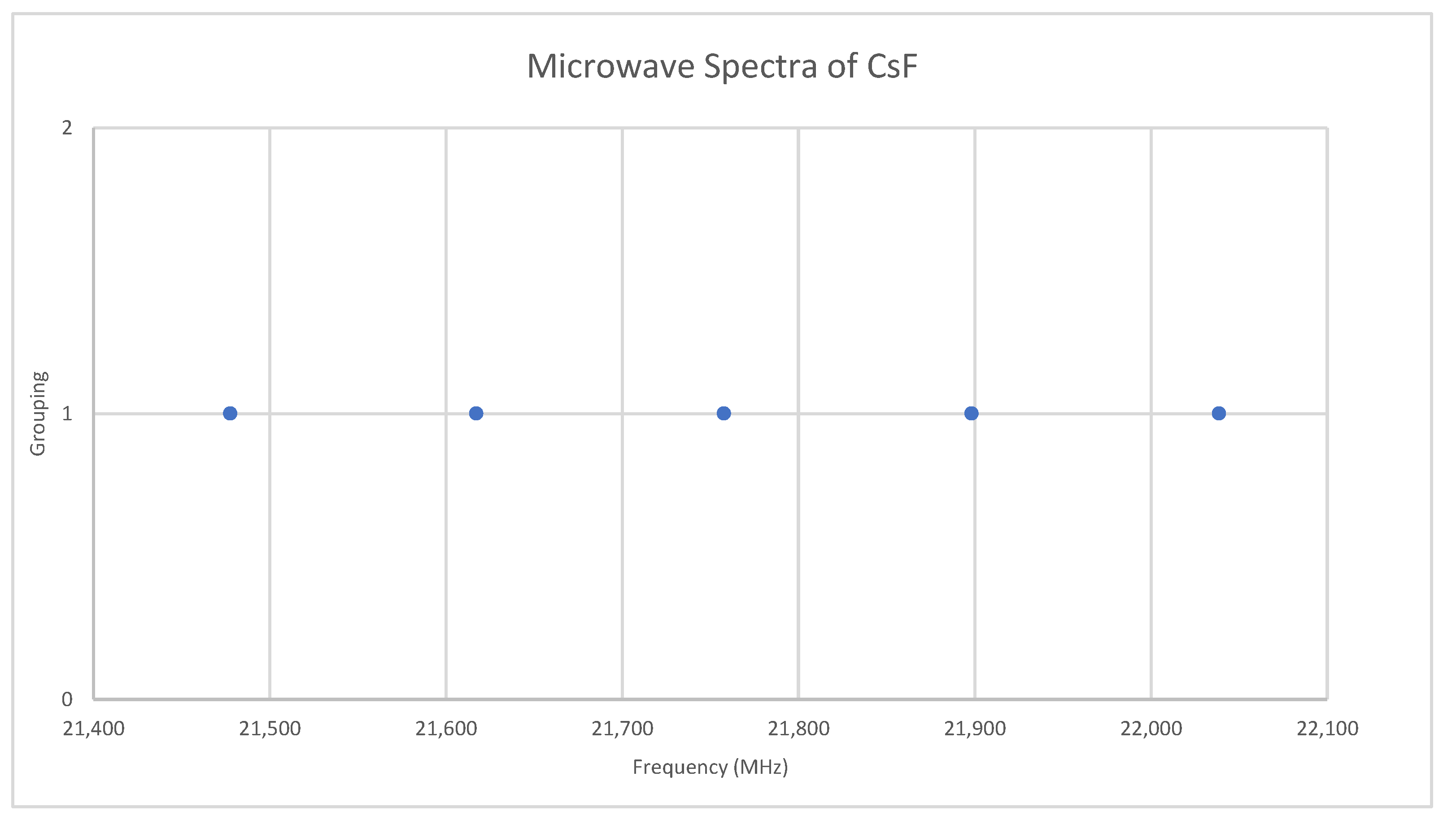
6.4. Cesium Fluoride (CsF)
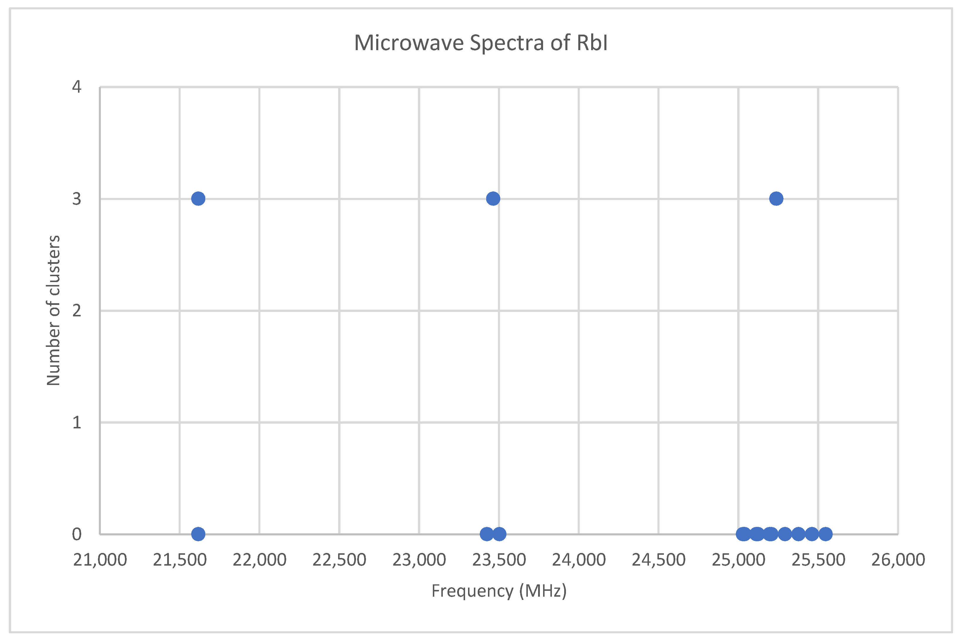
6.5. Rubidium Iodide (RbI)
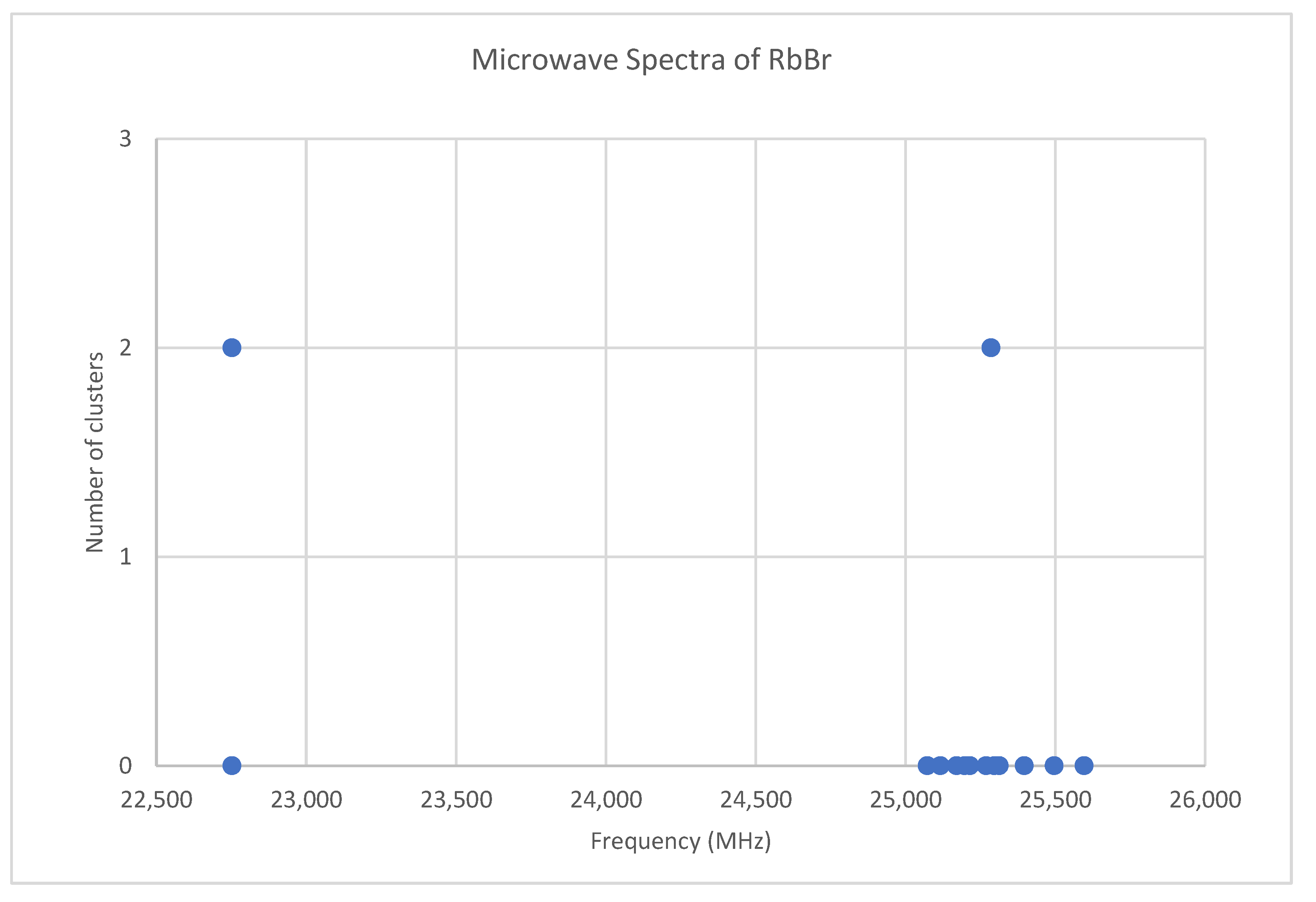
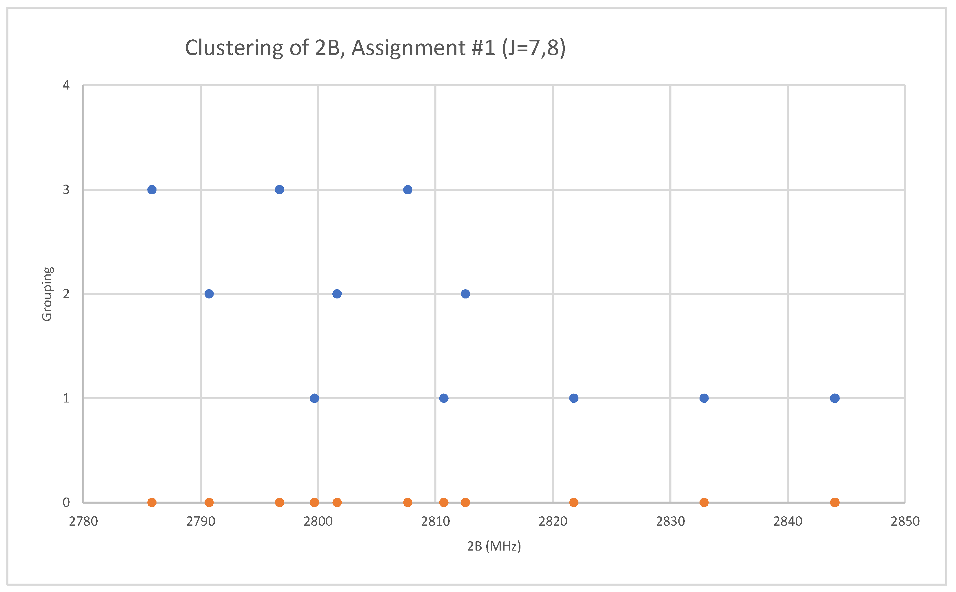
6.6. Rubidium Bromide (RbBr)
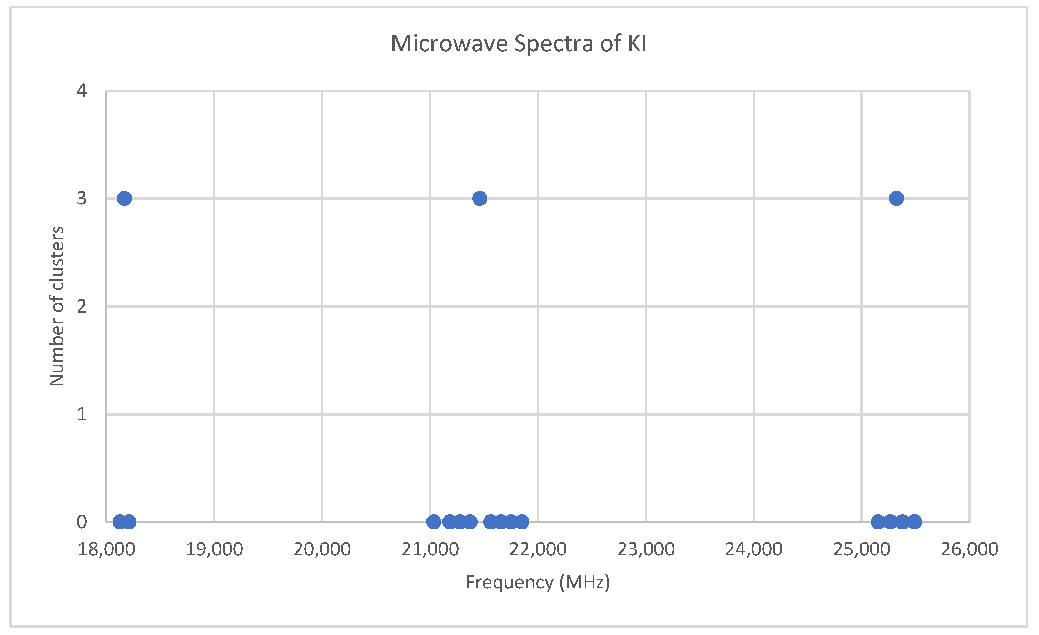
6.7. Potassium Iodide (KI)
6.8. Potassium Chloride (KCl)
6.9. Sodium Chloride (NaCl)
7. Conclusions
Supplementary Materials
Funding
Institutional Review Board Statement
Informed Consent Statement
Data Availability Statement
Acknowledgments
Conflicts of Interest
Appendix A. Analysis of the Microwave Spectrum of Cesium Fluoride (CsF)
Appendix B. Analysis of the Microwave Spectrum of Potassium Iodide (KI)
Appendix C. Analysis of the Microwave Spectrum of Potassium Chloride (KCl)
Appendix D. Analysis of the Microwave Spectrum of Potassium Chloride (KCl)
Appendix E. Analysis of the Microwave Spectrum of Sodium Chloride (NaCl)
References
- Ewing, G.W. Microwave Absorption Spectroscopy. J. Chem. Educ. 1966, 43, A683–A722. [Google Scholar]
- Townes, C.H.; Schawlow, A.L. Microwave Spectroscopy; Dover: New York, NY, USA, 1975. [Google Scholar]
- Schwendeman, R.H.; Volltrauer, H.N.; Laurie, V.W.; Thomas, E.C. Microwave Spectroscopy in the Undergraduate Laboratory. J. Chem. Educ. 1970, 47, 526–532. [Google Scholar]
- Dyke, T.R.; Muenter, J.S. A Stark Modulation Absorption Cell for Student Microwave Spectrometers. J. Chem. Educ. 1974, 51, 33. [Google Scholar] [CrossRef]
- Pollnow, G.F.; Hopfinger, A.J. A Computer Experiment in Microwave Spectroscopy. J. Chem. Educ. 1968, 45, 528–531. [Google Scholar] [CrossRef]
- Pollnow, G.F.; Chung, C.S.C. An Interactive Computer Program for Microwave Spectroscopy. J. Chem. Educ. 1973, 50, 794. [Google Scholar]
- McNaught, I.J.; Moore, R. Microwave Spectroscopy Tutor. J. Chem. Educ. 1995, 72, 993–994. [Google Scholar] [CrossRef]
- McNaught, I.J.; Moore, R. Winspec: A Microwave Spectroscopy Tutor. J. Chem. Educ. 1996, 73, 523.az. [Google Scholar]
- Woods, R.; Henderson, G. FTIR Rotational Spectroscopy. J. Chem. Educ. 1987, 64, 921–924. [Google Scholar] [CrossRef]
- McQuarrie, D.A. Quantum Chemistry, 2nd ed.; University Science Books: Herndon, VA, USA, 2008; Chapter 6. [Google Scholar]
- Pye, C.C. On the Solution of the Quantum Rigid Rotor. J. Chem. Educ. 2006, 83, 460–463. [Google Scholar] [CrossRef]
- Moynihan, C.T. Rationalization of the ΔJ=±1 Selection Rule for Rotational Transitions. J. Chem. Educ. 1969, 46, 431. [Google Scholar]
- Foss, J.G. Photonic Angular Momentum and Selection Rules for Rotational Transitions. J. Chem. Educ. 1970, 47, 778–779. [Google Scholar] [CrossRef]
- Chattaraj, P.K.; Sannigrahi, A.B. A Simple Group-Theoretical Derivation of the Selection Rules for Rotational Transitions. J. Chem. Educ. 1990, 67, 653–655. [Google Scholar]
- Laidler, K.J.; Meiser, J.H. Physical Chemistry, 3rd ed.; Houghton Mifflin: Boston, MA, USA, 1999; Chapter 13. [Google Scholar]
- Engel, T.; Reid, P. Physical Chemistry; Pearson: San Francisco, CA, USA, 2006; Chapter 19. [Google Scholar]
- House, J.E. Fundamentals of Quantum Mechanics; Academic Press: San Diego, CA, USA, 1998; Chapter 7. [Google Scholar]
- Ratner, M.A.; Schatz, G.C. Introduction to Quantum Mechanics in Chemistry; Prentice-Hall: Upper Saddle River, NJ, USA, 2001; Chapter 4. [Google Scholar]
- Atkins, P.; de Paula, J. Physical Chemistry, 10th ed.; Freeman: New York, NY, USA, 2014; Chapter 12. [Google Scholar]
- Berry, R.S.; Rice, S.A.; Ross, J. Physical Chemistry, 2nd ed.; Oxford University Press: New York, NY, USA, 2000; Chapter 7. [Google Scholar]
- Alberty, R.A.; Silbey, R.J. Physical Chemistry, 2nd ed.; Wiley: New York, NY, USA, 1997; Chapter 13. [Google Scholar]
- Mortimer, R.G. Physical Chemistry, 2nd ed.; Harcourt: San Diego, CA, USA, 2000; Chapter 19. [Google Scholar]
- Zielinski, T.J. Fostering Creativity and Learning Using Instructional Symbolic Mathematics Documents. J. Chem. Educ. 2009, 86, 1466–1467. [Google Scholar]
- Microsoft Office Professional Plus (Excel) 2016, Microsoft Corporation: Redmond, WA, USA, 2016.
- Solver, Microsoft Office Add-In, Frontline Systems: Incline Village, NV, USA, 2016.
- Gilliam, O.R.; Johnson, C.M.; Gordy, W. Microwave Spectroscopy in the Region from Two to Three Millimeters. Phys. Rev. 1950, 78, 140–144. [Google Scholar]
- Vegard, L. Struktur und Leuchtfahigkeit von festem Kohlenoxyd. Z. Phys. 1930, 61, 185–190. [Google Scholar] [CrossRef]
- Crystallography Open Database. Available online: http://www.crystallography.net (accessed on 31 March 2018).
- Wyckoff, R.W.G. Crystal Structures; Wiley: New York, NY, USA, 1963; Chapter 3; pp. 85–237. [Google Scholar]
- Maxwell, L.R.; Hendricks, S.B.; Mosley, V.M. Interatomic Distances of the Alkali Halide Molecules by Electron Diffraction. Phys. Rev. 1937, 52, 968–972. [Google Scholar]
- Honig, A.; Mandel, M.; Stitch, M.L.; Townes, C.H. Microwave Spectra of the Alkali Halides. Phys. Rev. 1954, 96, 629–642. [Google Scholar] [CrossRef]
- Pye, C.C. One-Dimensional Cluster Analysis and its Application to Chemistry. Chem. Educ. 2020, 25, 50–57. [Google Scholar]
- Pye, C.C. Intuitive Solution to Quantum Harmonic Oscillator at Infinity. J. Chem. Educ. 2004, 81, 830–831. [Google Scholar]
- McHale, J.L. Molecular Spectroscopy; Prentice-Hall: Upper Saddle River, NJ, USA, 1999; Chapters 8–9. [Google Scholar]
- Dykstra, C.E. Introduction to Quantum Chemistry; Prentice-Hall: Englewood Cliffs, NJ, USA, 1994; Chapter 5. [Google Scholar]
- Hollenberg, J.L. Energy States of Molecules. J. Chem. Educ. 1970, 47, 2–14. [Google Scholar] [CrossRef]
- Brown, J.M. Molecular Spectroscopy; Oxford Science Publications: Oxford, UK, 1999; Chapter 5. [Google Scholar]
- Stitch, M.L.; Honig, A.; Townes, C.H. Microwave Spectra at High Temperature—Spectra of CsCl and NaCl. Phys. Rev. 1952, 86, 813–814. [Google Scholar] [CrossRef]
- Stitch, M.L.; Honig, A.; Townes, C.H. High Temperature Microwave Spectroscopy—Spectrum of KCl, TlCl. Phys. Rev. 1952, 86, 607. [Google Scholar]
- Tate, P.A.; Strandberg, M.W.P. Stark Effect in the Microwave Spectra of KCl and NaCl. J. Chem. Phys. 1954, 22, 1380–1383. [Google Scholar] [CrossRef]


| MX | R (Å) 1 | R (Å) 4 | Ratio |
|---|---|---|---|
| LiF | 2.0086 | ||
| LiCl | 2.56477 | ||
| LiBr | 2.7506 | ||
| LiI | 3.000 | ||
| NaF | 2.310 | ||
| NaCl | 2.8203 | 2.51 | 1.124 |
| NaBr | 2.98662 | 2.64 | 1.131 |
| NaI | 3.2364 | 2.90 | 1.116 |
| KF | 2.6735 | ||
| KCl | 3.14647 | 2.79 | 1.128 |
| KBr | 3.3000 | 2.94 | 1.122 |
| KI | 3.53278 | 3.23 | 1.093 |
| RbF | 2.82 | ||
| RbCl | 3.2905 | 2.89 | 1.139 |
| RbBr | 3.427 | 3.06 | 1.120 |
| RbI | 3.671 | 3.26 | 1.126 |
| CsF | 3.004 | ||
| CsCl | 3.51 2 | 3.06 | 1.147 |
| 3.5706 3 | 1.167 | ||
| CsBr | 3.7118 3 | 3.14 | 1.182 |
| CsI | 3.9549 3 | 3.41 | 1.159 |
| Model | Be | αe | γe | De1 | SSE |
|---|---|---|---|---|---|
| 1 | 708.266 | 2.040 | n/a | n/a | 0.7213 |
| 2 | 708.269 | 2.045 | 0.0015 | n/a | 0.6840 |
| 3 | 708.280 | 2.040 | n/a | 25.7 | 0.5194 |
| 4 | 708.362 | 2.043 | 0.0011 | 162 | 0.0102 |
| Model | Be | αe | γe | De1 | SSE | |
|---|---|---|---|---|---|---|
| 133Cs79Br | 1 | 1081.242 | 3.692 | n/a | n/a | 3.998 |
| 2 | 1081.283 | 3.720 | 0.0033 | n/a | 1.426 | |
| 3 | 1081.281 | 3.692 | n/a | −0.162 | 2.520 | |
| 4 | 1081.313 | 3.718 | 0.0030 | −0.138 | 0.361 | |
| 133Cs81Br | 1 | 1064.512 | 3.617 | n/a | n/a | 0.263 |
| 2 | 1064.521 | 3.632 | 0.0032 | n/a | 0.177 | |
| 3 | 1064.538 | 3.618 | n/a | −0.097 | 0.130 | |
| 4 | 1064.552 | 3.635 | 0.0037 | −0.107 | 0.018 |
| Model | Be | αe | γe | SSE | |
|---|---|---|---|---|---|
| 133Cs35Cl [38], n = 4 | 1 | 2163.119 | 9.963 | n/a | 0.115 |
| [31], n = 9 | 1 | 2161.029 | 10.021 | n/a | 4.195 |
| 2 | 2161.152 | 10.10 | 0.0091 | 0.522 | |
| 133Cs37Cl [38], n = 4 | 1 | 2071.458 | 9.600 | n/a | 8.940 |
| 2 | 2071.155 | 9.238 | −0.0703 | 0.002 | |
| [31], n = 3 | 1 | 2068.713 | 9.436 | n/a | 0.035 |
| 2 | 2068.682 | 9.378 | −0.0192 | exact |
| Model | Be | αe | γe | De1 | SSE | |
|---|---|---|---|---|---|---|
| 85Rb127I | 1 | 984.221 | 3.261 | n/a | n/a | 1.013 |
| 2 | 984.245 | 3.284 | 0.0033 | n/a | 0.237 | |
| 3 | 984.307 | 3.259 | n/a | 289 | 0.644 | |
| 4 | 984.236 | 3.279 | 0.0027 | −81 | 0.113 | |
| 87Rb127I | 1 | 970.681 | 3.204 | n/a | n/a | 0.014 |
| 2 | 970.672 | 3.188 | −0.0056 | n/a | exact |
| Model | Be | αe | γe | De1 | SSE | |
|---|---|---|---|---|---|---|
| 85Rb79Br | 1 | 1424.768 | 5.542 | n/a | n/a | 0.432 |
| 2 | 1424.798 | 5.583 | 0.0086 | n/a | 0.041 | |
| 3 | 1424.822 | 5.538 | n/a | −0.79 | 0.268 | |
| 4 | 1424.822 | 5.576 | 0.0076 | −0.40 | 0.005 | |
| 87Rb79Br | 1 | 1409.003 | 5.456 | n/a | n/a | 0.011 |
| 2 | 1409.014 | 5.478 | 0.0072 | n/a | exact | |
| 85Rb81Br | 1 | 1406.546 | 5.450 | n/a | n/a | 0.020 |
| 2 | 1406.562 | 5.479 | 0.0097 | n/a | exact |
Disclaimer/Publisher’s Note: The statements, opinions and data contained in all publications are solely those of the individual author(s) and contributor(s) and not of MDPI and/or the editor(s). MDPI and/or the editor(s) disclaim responsibility for any injury to people or property resulting from any ideas, methods, instructions or products referred to in the content. |
© 2023 by the author. Licensee MDPI, Basel, Switzerland. This article is an open access article distributed under the terms and conditions of the Creative Commons Attribution (CC BY) license (https://creativecommons.org/licenses/by/4.0/).
Share and Cite
Pye, C.C. Interpreting the Microwave Spectra of Diatomic Molecules. Spectrosc. J. 2023, 1, 3-27. https://doi.org/10.3390/spectroscj1010002
Pye CC. Interpreting the Microwave Spectra of Diatomic Molecules. Spectroscopy Journal. 2023; 1(1):3-27. https://doi.org/10.3390/spectroscj1010002
Chicago/Turabian StylePye, Cory C. 2023. "Interpreting the Microwave Spectra of Diatomic Molecules" Spectroscopy Journal 1, no. 1: 3-27. https://doi.org/10.3390/spectroscj1010002
APA StylePye, C. C. (2023). Interpreting the Microwave Spectra of Diatomic Molecules. Spectroscopy Journal, 1(1), 3-27. https://doi.org/10.3390/spectroscj1010002