
High-Frequency Flow Rate Determination—A Pressure-Based Measurement Approach


Abstract
:1. Introduction
2. Materials and Methods
2.1. Volumetric Flow Rate Measurement Methods
2.2. Transient Flow Rate Models
2.3. Analytical Soft Sensor Model for Flow Rate Calculation
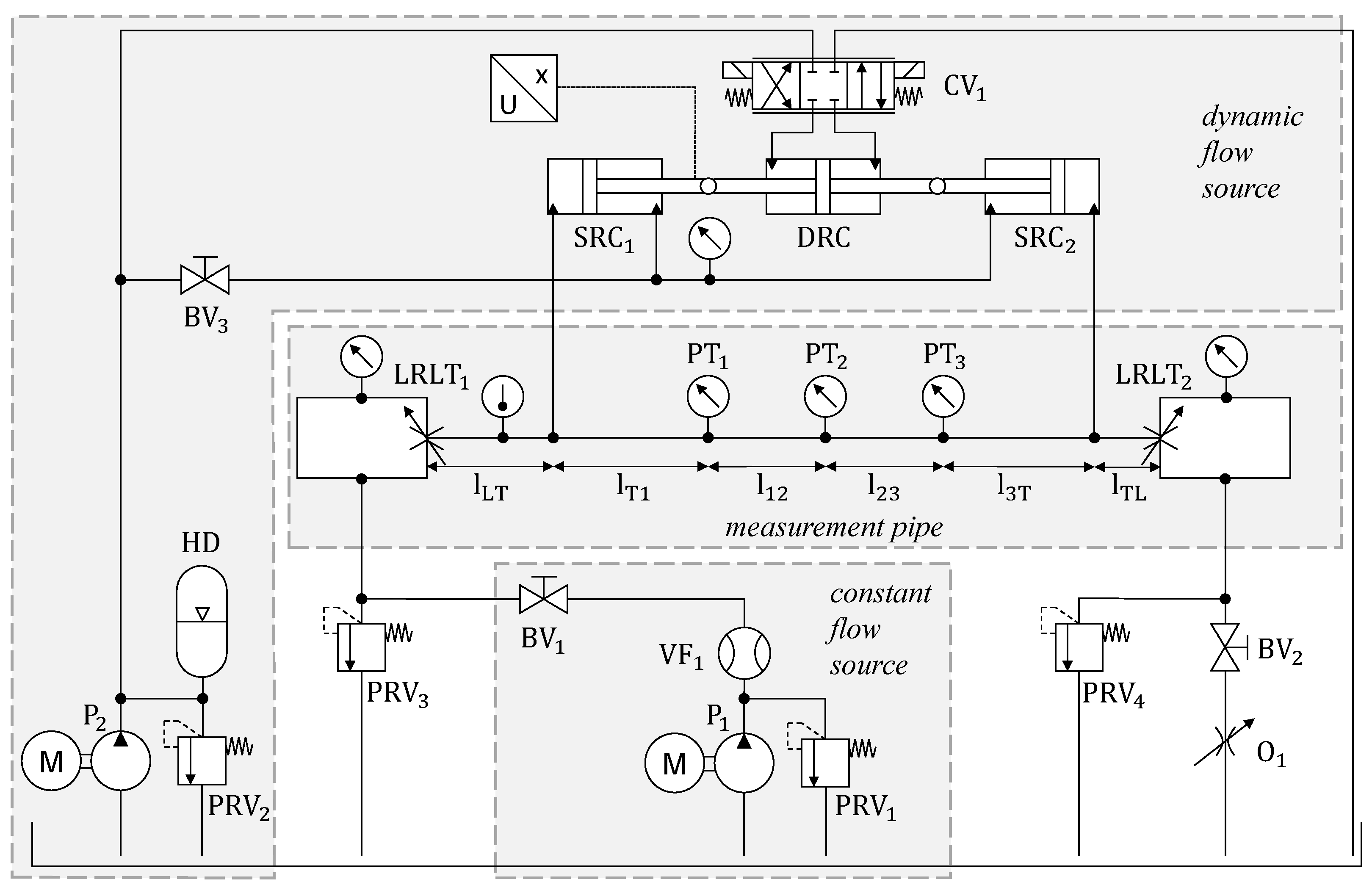
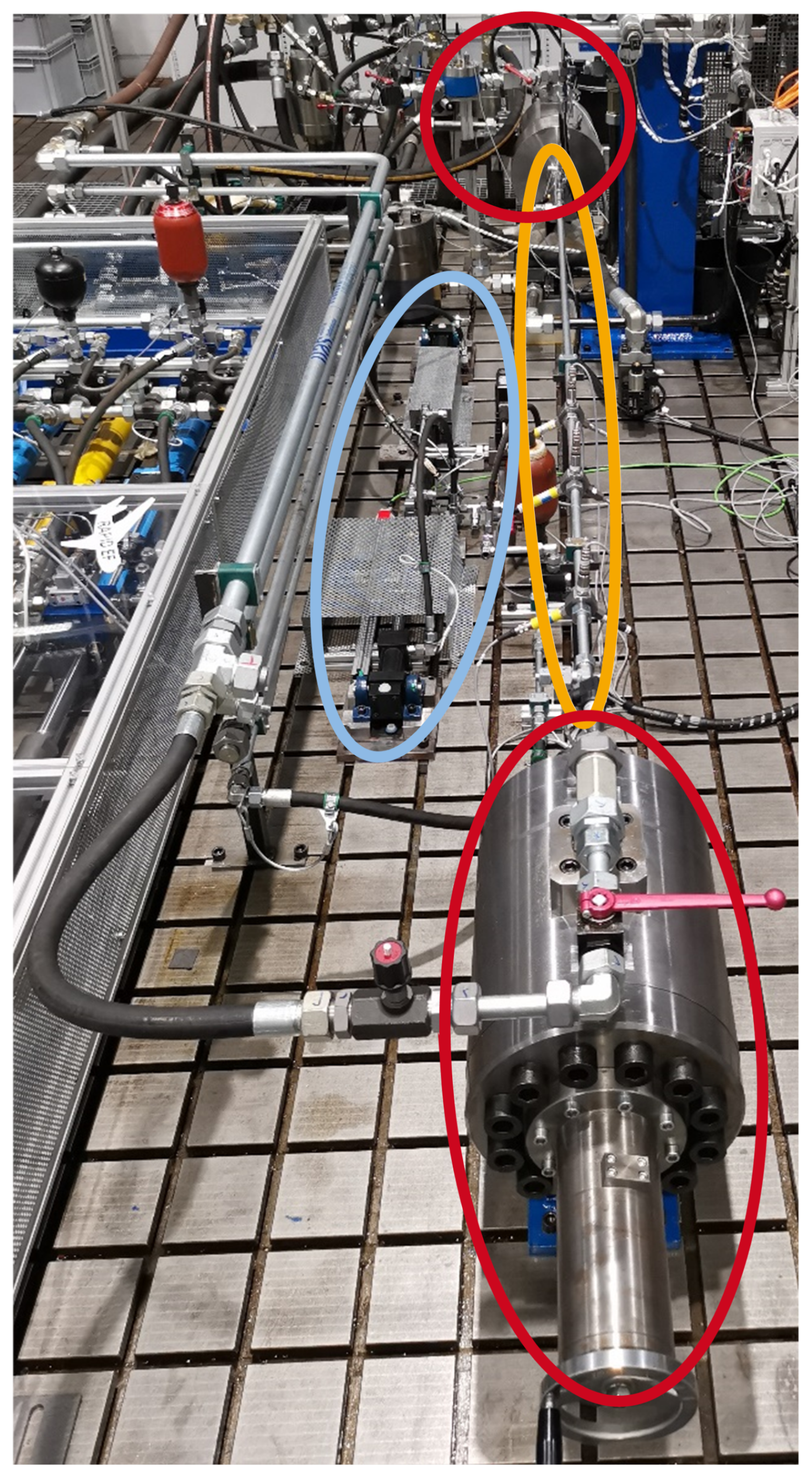
2.4. Test Rig
2.5. Test Cases
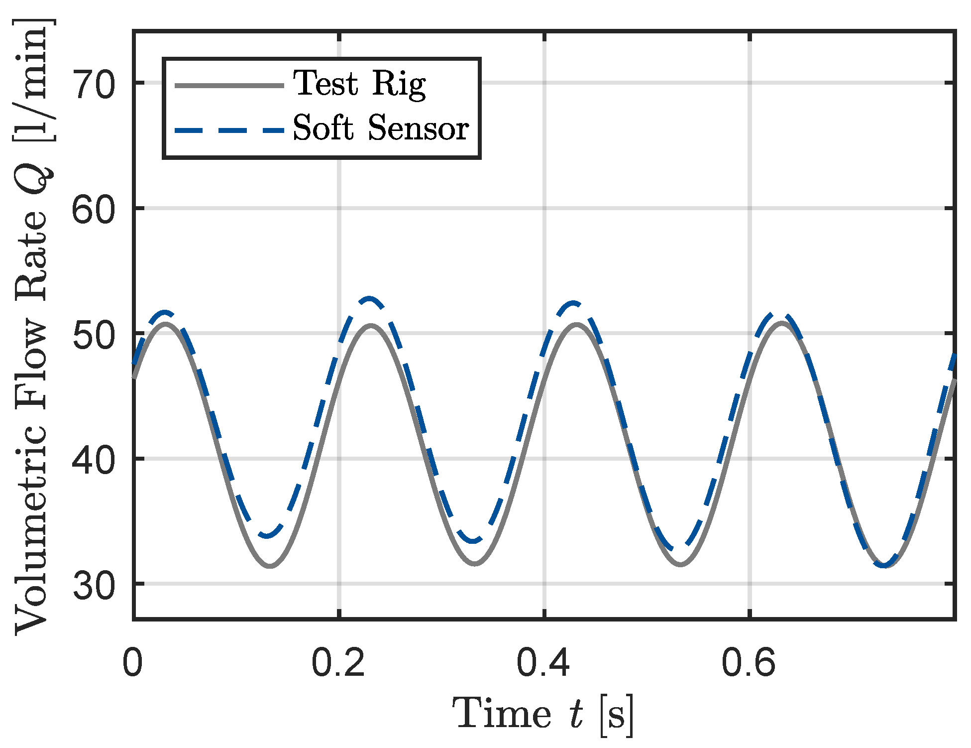
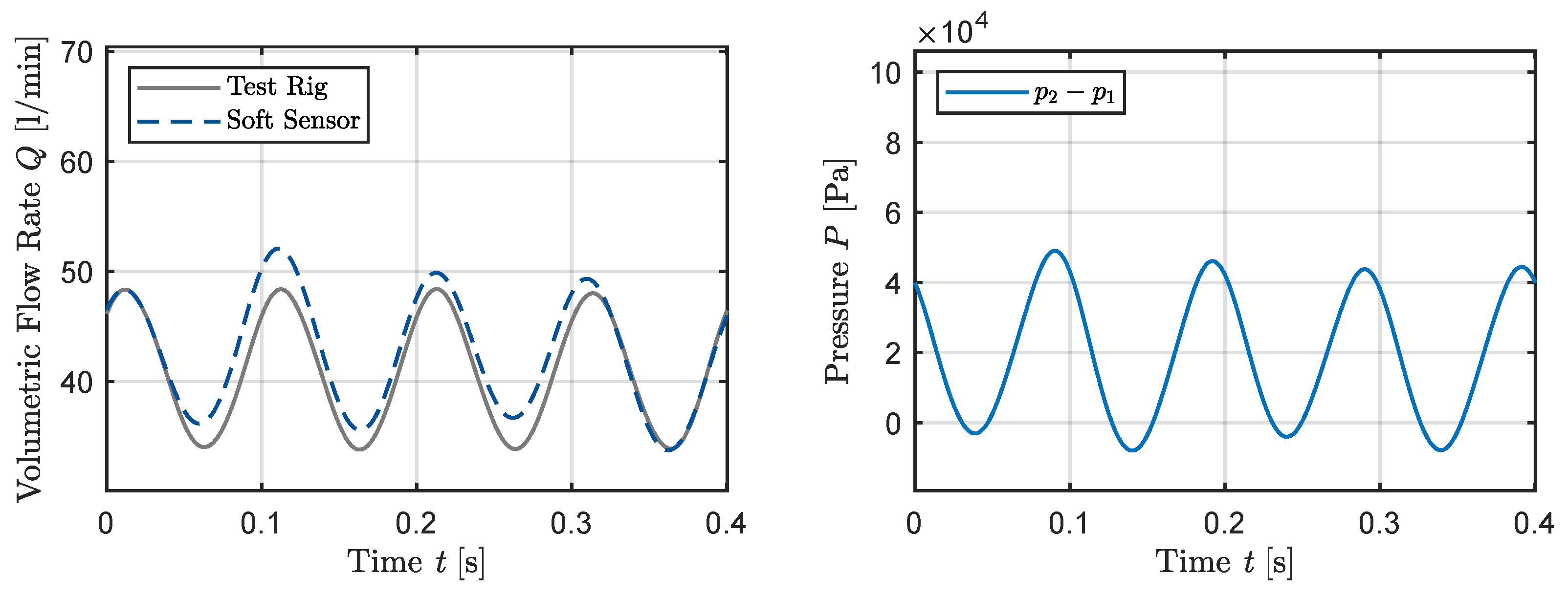
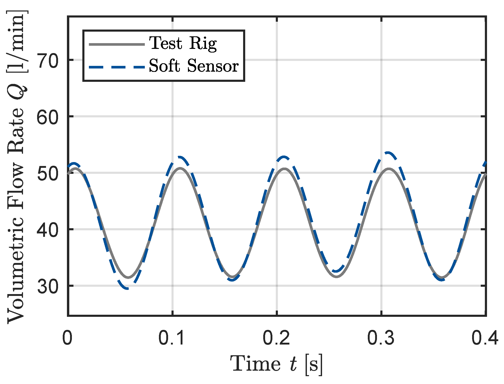
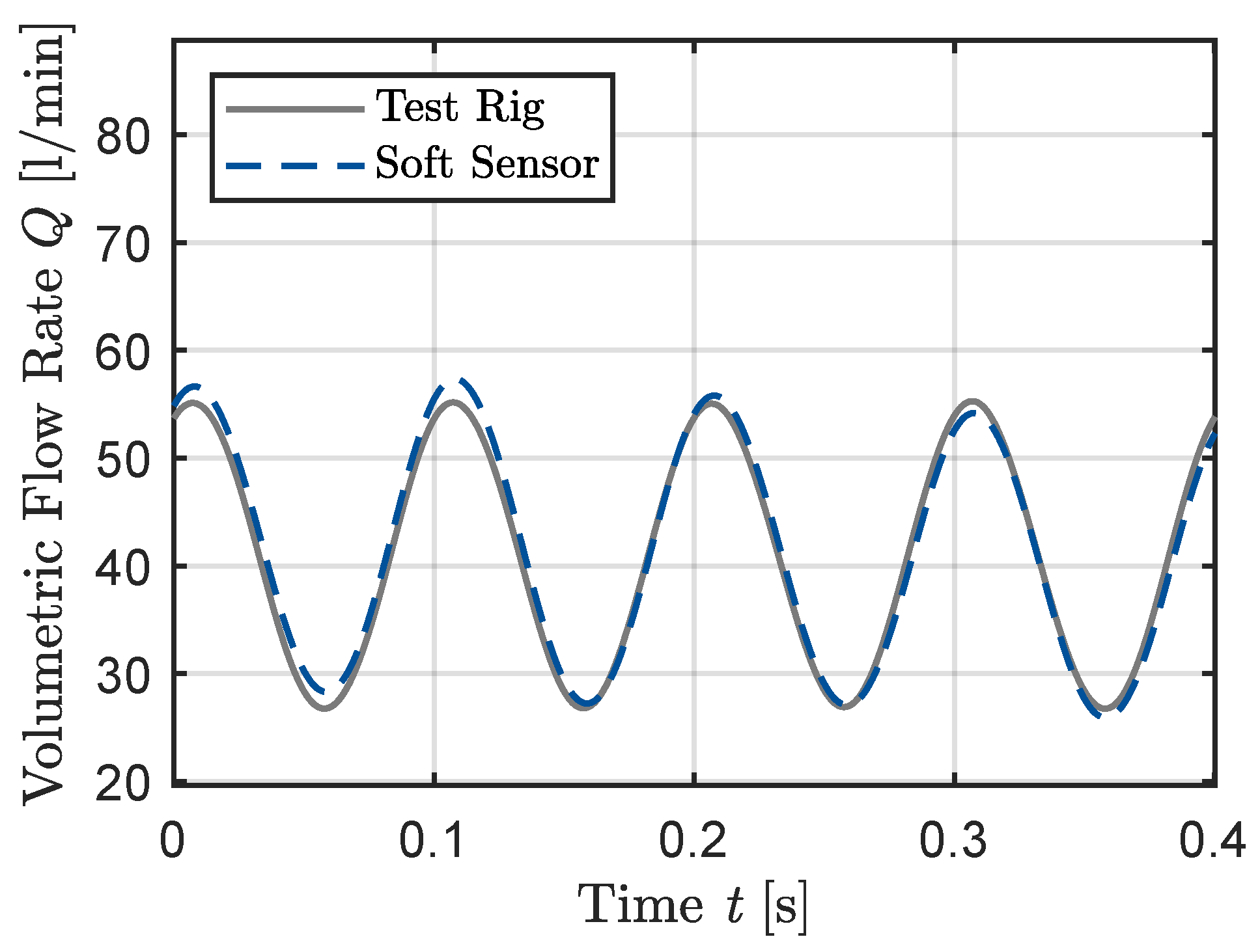
3. Results


4. Discussion
5. Conclusions
Author Contributions
Funding
Institutional Review Board Statement
Informed Consent Statement
Data Availability Statement
Conflicts of Interest
Abbreviations
| BV | Ball Valve |
| CV | Control Valve |
| DRC | Double-rod Cylinder |
| HD | Hydraulic Damper |
| HP | Hagen and Poiseuille |
| HWA | Hot-wire Anemometry |
| ILT | Inverse Laplace transformation |
| LRLT | Low-reflection line terminator |
| O | Adjustable Orifice |
| P | Hydraulic Pump |
| PIV | Particle Image Velocimetry |
| PT | Pressure Transducer |
| Re | Reynolds number |
| SRC | Single-rod Cylinder |
| SV | Switching Valve |
| VF | Volumetric Flow Rate Sensor |
Nomenclature
| Symbol | Definition | Unit |
| * | Denotation of a Variable in the Laplace Domain | [m2/s] |
| a | Speed of Sound | [m/s] |
| A | Cross-section of the Cylinder | [m2] |
| Geometric Parameter | [m2] | |
| Cross-section of the Pipe | [m2] | |
| Dissipation Number | [-] | |
| f | Frequency | [Hz] |
| Propagation Operator | [-] | |
| Modified Bessel function of the first kind of the i’th order | [-] | |
| K | Isentropic Bulk Modulus | [Pa] |
| First part of the convolution integral | [-] | |
| Second part of the convolution integral | [-] | |
| Approximation of | [-] | |
| k | A Natural Number | [-] |
| l | Pipe section length | [m] |
| L | Length of the Pipe | [m] |
| m | Order of poles | [-] |
| Part of Assumed Weighting Function | [-] | |
| Part of Assumed Weighting Function | [-] | |
| N | Upper Limit of Residue Sum | [-] |
| Pressure Difference | [-] | |
| System Pressure | [bar] | |
| Pressure at Inlet | [bar] | |
| Pressure at Outlet | [bar] | |
| Q | Volumetric Flow Rate | [m3/s] |
| Volumetric Flow Rate from the Cylinder | [m3/s] | |
| Mean Volumetric Flow Rate | [m3/s] | |
| Maximum Volumetric Flow Rate | [m3/s] | |
| Minimum Volumetric Flow Rate | [m3/s] | |
| Stationary Volumetric Flow Rate | [m3/s] | |
| Volumetric flow rate at Inlet: and Outlet: | [m3/s] | |
| r | Radial Coordinate of the Pipe | [m] |
| R | Radius of the Pipe | [m] |
| Reynolds Number | [-] | |
| Hydraulic Resistance | [Pa/(m3/s)] | |
| s | Laplace Variable | [-] |
| Approximation of the Function | [-] | |
| t | Time | [s] |
| Normalized Time | [-] | |
| v | Velocity of the Cylinder | [m/s] |
| Axial Velocity | [m/s] | |
| Weighting function at End of the Pipe | [-] | |
| Weighting function at port | [-] | |
| Negative of | [-] | |
| Compressible Weighting Function at port 1 | [-] | |
| Incompressible Weighting Function | [-] | |
| Womersley Number | [-] | |
| x | Axial Coordinate of the Pipe | [m] |
| z | Number of Pistons of an Axial Piston Pump | [-] |
| Discharge Coefficient | [-] | |
| Degree of Non-uniformity | [-] | |
| Normalized Laplace Variable | [-] | |
| Poles of the Weighting Function | [Pas] | |
| Series impedance | [] | |
| Dynamic Viscosity | [Pas] | |
| Kinematic Viscosity | [m2/s] | |
| Pressure Variation Frequency | [1/s] | |
| Fluid Density | [kg/m3] | |
| Normalized Time | [s] |
Appendix A. Derivation
Appendix A.1. Setup of the Problem
- The flow is laminar (Reynolds number ), which means that the fluid layers do not mix. Therefore, the pressure gradient in the radial direction is negligible because the pressure remains constant across the pipe’s cross-section.
- There is axisymmetry in the flow and pipe geometry; therefore, the gradient in the angular direction is zero, i.e., .
- The velocity in the axial coordinate is much less than the speed of sound a. Therefore, , and the Mach number , and supersonic effects can be ignored.
- The pipe length is big in relation to its radius (). Therefore, there are no pressure reflections at the pipe walls.
- The significant viscous effects in the motion equations are limited to those involving the radial distribution of axial velocity [26].
- The pipe is horizontal, so gravitation is negligible as the forces are constant over the pipes’ length.
- The fluid density is constant over the vertical position within the pipe because the pipe’s diameter is small.
- Heat transfer is ignored since the focus is on liquids, excluding gases [37].
Appendix A.2. Derivation of the Inverse Laplace Transformed Weighting Functions
- .
Appendix B. Test Rig Details
Appendix B.1. Low-Reflection Line Terminator


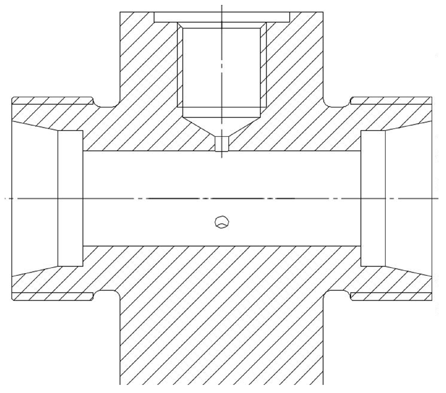
Appendix B.2. Pressure Transducer Installation
References
- Sutera, S.P.; Skalak, R. The History of Poiseuille’s Law. Annu. Rev. Fluid Mech. 1993, 25, 1–20. [Google Scholar] [CrossRef]
- Richardson, E.G.; Tyler, E. The transverse velocity gradient near the mouths of pipes in which an alternating or continuous flow of air is established. Proc. Phys. Soc. 1929, 42, 1–15. [Google Scholar] [CrossRef]
- Manhartsgruber, B. Instantaneous Liquid Flow Rate Measurement Utilizing the Dynamics of Laminar Pipe Flow. J. Fluids Eng. 2008, 130, 121402. [Google Scholar] [CrossRef]
- Kashima, A.; Lee, P.; Ghidaoui, M. A selective literature review of methods for measuring the flow rate in pipe transient flows. In Proceedings of the BHR Group—11th International Conferences on Pressure Surges, Lisbon, Portugal, 24–26 October 2012; pp. 733–742. [Google Scholar]
- Wiklund, D.; Peluso, M. Quantifying and Specifying the Dynamic Response of Flowmeters. Conf. ISA 2002, 422, 463–476. [Google Scholar]
- Mottram, R. Introduction: An overview of pulsating flow measurement. Flow Meas. Instrum. 1992, 3, 114–117. [Google Scholar] [CrossRef]
- Ligeza, P. Static and dynamic parameters of hot-wire sensors in a wide range of filament diameters as a criterion for optimal sensor selection in measurement process. Measurement 2020, 151, 107177. [Google Scholar]
- Duensing, Y.; Richert, O.; Schmitz, K. Investigating the Condition Monitoring Potential of Oil Conductivity for Wear Identification in Electro Hydrostatic Actuators. In Proceedings of the ASME/Bath 2021 Symposium on Fluid Power and Motion Control, Online, 19–21 October 2021. [Google Scholar]
- Brunone, B.; Berni, A. Wall Shear Stress in Transient Turbulent Pipe Flow by Local Velocity Measurement. J. Hydraul. Eng. 2010, 136, 716–726. [Google Scholar] [CrossRef]
- Grant, I. Particle image velocimetry: A review. Proc. Inst. Mech. Eng. Part C J. Mech. Eng. Sci. 1997, 211, 55–76. [Google Scholar]
- Henry, M.; Zamora, M. The dynamic response of Coriolis mass flow meters: Theory and applications. Tech. Pap. ISA 2004, 454. [Google Scholar]
- Hucko, S.; Krampe, H.; Schmitz, K. Evaluation of a Soft Sensor Concept for Indirect Flow Rate Estimation in Solenoid-Operated Spool Valves. Actuators 2023, 12, 148. [Google Scholar] [CrossRef]
- Brumand-Poor, F.; Kotte, T.; Pasquini, E.; Kratschun, F.; Enking, J.; Schmitz, K. Unsteady flow rate in transient, incompressible pipe flow. Z. Angew. Math. Mech. 2024, e202300125. [Google Scholar] [CrossRef]
- Brumand-Poor, F.; Kotte, T.; Pasquini, E.; Schmitz, K. Signal Processing for High-Frequency Flow Rate Determination: An Analytical Soft Sensor Using Two Pressure Signals. Signals 2024, 5, 812–840. [Google Scholar] [CrossRef]
- Brereton, G.J.; Schock, H.J.; Rahi, M.A.A. An indirect pressure-gradient technique for measuring instantaneous flow rates in unsteady duct flows. Exp. Fluids 2006, 40, 238–244. [Google Scholar] [CrossRef]
- Brereton, G.J.; Schock, H.J.; Bedford, J.C. An indirect technique for determining instantaneous flow rate from centerline velocity in unsteady duct flows. Flow Meas. Instrum. 2008, 19, 9–15. [Google Scholar] [CrossRef]
- Sundstrom, L.R.J.; Saemi, S.; Raisee, M.; Cervantes, M.J. Improved frictional modeling for the pressure-time method. Flow Meas. Instrum. 2019, 69, 101604. [Google Scholar] [CrossRef]
- Foucault, E.; Szeger, P. Unsteady flowmeter. Flow Meas. Instrum. 2019, 69, 101607. [Google Scholar] [CrossRef]
- García García, F.J.; Fariñas Alvariño, P. On an analytic solution for general unsteady/transient turbulent pipe flow and starting turbulent flow. Eur. J. Mech.-B/Fluids 2019, 74, 200–210. [Google Scholar] [CrossRef]
- García García, F.J.; Fariñas Alvariño, P. On the analytic explanation of experiments where turbulence vanishes in pipe flow. J. Fluid Mech. 2022, 951, A4. [Google Scholar] [CrossRef]
- Urbanowicz, K.; Bergant, A.; Stosiak, M.; Deptuła, A.; Karpenko, M. Navier-Stokes Solutions for Accelerating Pipe Flow—A Review of Analytical Models. Energies 2023, 16, 1407. [Google Scholar] [CrossRef]
- Urbanowicz, K.; Bergant, A.; Stosiak, M.; Karpenko, M.; Bogdevičius, M. Developments in analytical wall shear stress modelling for water hammer phenomena. J. Sound Vib. 2023, 562, 117848. [Google Scholar] [CrossRef]
- Bayle, A.; Rein, F.; Plouraboué, F. Frequency varying rheology-based fluid–structure-interactions waves in liquid-filled visco-elastic pipes. J. Sound Vib. 2023, 562, 117824. [Google Scholar] [CrossRef]
- Bayle, A.; Plouraboue, F. Laplace-Domain Fluid–Structure Interaction Solutions for Water Hammer Waves in a Pipe. J. Hydraul. Eng. 2024, 150, 04023062. [Google Scholar] [CrossRef]
- Brumand-Poor, F.; Schüpfer, M.; Merkel, A.; Schmitz, K. Development of a Hydraulic Test Rig for a Virtual Flow Sensor. In Proceedings of the Eighteenth Scandinavian International Conference on Fluid Power (SICFP’23), Tampere, Finland, 30 May–1 June 2023. [Google Scholar]
- Stecki, J.S.; Davis, D.C. Fluid Transmission Lines—Distributed Parameter Models Part 1: A Review of the State of the Art. Proc. Inst. Mech. Eng. Part A Power Process. Eng. 1986, 200, 215–228. [Google Scholar] [CrossRef]
- Almondo, A.; Sorli, M. Time Domain Fluid Transmission Line Modelling using a Passivity Preserving Rational Approximation of the Frequency Dependent Transfer Matrix. Int. J. Fluid Power 2006, 7, 41–50. [Google Scholar] [CrossRef]
- Weber, H.; Ulrich, H. Laplace-, Fourier- und z-Transformation; Vieweg+Teubner Verlag: Wiesbaden, Germany, 2012. [Google Scholar] [CrossRef]
- Dietmar Findeisen, S.H. Ölhydraulik—Handbuch der hydraulischen Antriebe und Steuerungen; Springer: Berlin/Heidelberg, Germany, 2015. [Google Scholar]
- Will, D.; Gebhardt, N.; Nollau, R.; Herschel, D. Hydraulik: Grundlagen, Komponenten, Schaltungen; Springer: Berlin/Heidelberg, Germany, 2008. [Google Scholar]
- D’Souza, A. Dynamic Response of Fluid Lines. J. Basic Eng. 1964, 86, 589–598. [Google Scholar] [CrossRef]
- Gong, J.; Lambert, M.; Zecchin, A.; Simpson, A. Experimental verification of pipeline frequency response extraction and leak detection using the inverse repeat signal. J. Hydraul. 2016, 54, 210–219. [Google Scholar] [CrossRef]
- Schmitz, K.; Murrenhoff, H. Hydraulik; Vollständig neu Bearbeitete Auflage; Reihe Fluidtechnik. U; Shaker Verlag: Aachen, Germany, 2018; Volume 002. [Google Scholar]
- Butterworth, S. On the Theory of Filter Amplifiers. Exp. Wirel. Wirel. Eng. 1930, 7, 536–541. [Google Scholar]
- The MathWorks Inc. MATLAB, version: 9.13.0 (R2022b); The MathWorks Inc.: Natick, MA, USA, 2022. [Google Scholar]
- Brumand-Poor, F.; Kotte, T.; Abdulaziz, H.; Reese, C.; Schmitz, K. Advancing Pressure-Based Flow Rate Soft Sensors: Signal Filtering Effects and Non-Laminar Flow Rate Determination. Preprints 2024. [Google Scholar] [CrossRef]
- Brown, F.T.; Nelson, S.E. Step Responses of Liquid Lines with Frequency-Dependent Effects of Viscosity. J. Basic Eng. 1965, 87, 504–510. [Google Scholar] [CrossRef]
- Krantz, S.G. Handbook of Complex Variables; Birkhäuser: Boston, MA, USA, 1999. [Google Scholar]
- Goodson, R.E. Distributed system simulation using infinite product expansions. Simulation 1970, 15, 255–263. [Google Scholar] [CrossRef]
- Maple; Maplesoft, a Division of Waterloo Maple Inc., ON, Canada, 2019. 2023. Available online: https://www.maplesoft.com/products/Maple/ (accessed on 20 July 2023).

| Test Case | System Pressure [bar] | Mean Volumetric Flow Rate [L/min] | Degree of Non-Uniformity [-] | Frequency f [Hz] |
|---|---|---|---|---|
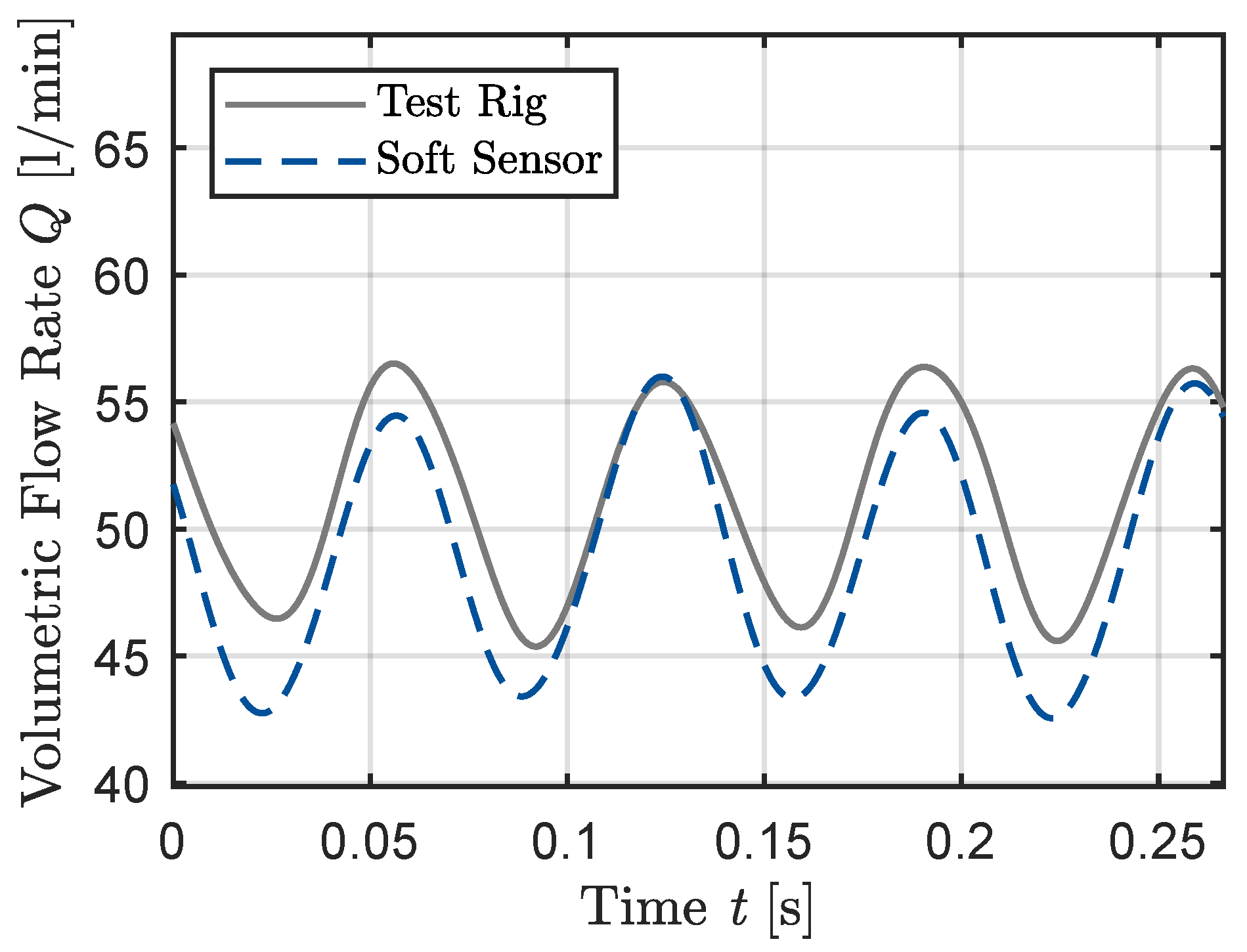
| Sine (Figure 3, Figure 4 and Figure 5) | 100 | 40 | , , | 5 |
| Sine (Figure 6, Figure 7 and Figure 8) | 100 | 40 | , , | 10 |
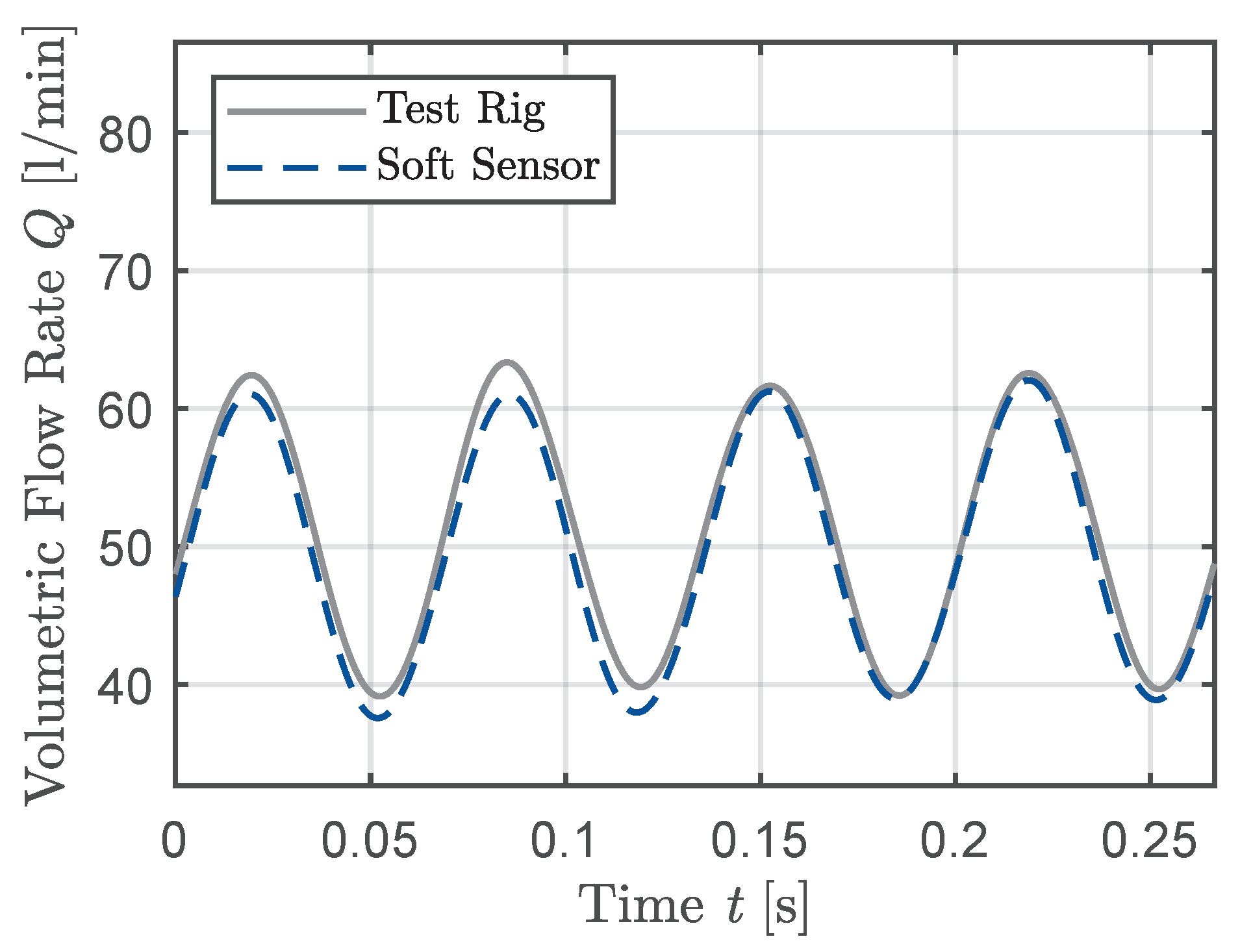
| Sine (Figure 9, Figure 10 and Figure 11) | 100 | 50 | , , | 15 |
| Frequency f [Hz] | Degree of Non-Uniformity [-] | Mean Absolute Error | Standard Deviation | Max Absolute Error |
|---|---|---|---|---|
| 5 (Figure 3, Figure 4 and Figure 5) | , , | , , | , , | , , 13 |
| 10 (Figure 6, Figure 7 and Figure 8) | , , | , , | , , | 10, , |
| 15 (Figure 9, Figure 10 and Figure 11) | , , | , , | , , | 9, 8, |
| Frequency f [Hz] | Degree of Non-Uniformity [-] | Mean Absolute Error HP | Standard Deviation HP | Max Absolute Error HP |
|---|---|---|---|---|
| 5 (Figure 3, Figure 4 and Figure 5) | , , | , , | 44, , | , 112, 158 |
| 10 (Figure 6, Figure 7 and Figure 8) | , , | , 135, 179 | , 151, 201 | 164, 228, 317 |
| 15 (Figure 9, Figure 10 and Figure 11) | , , | , 127, 172 | , 141, 191 | 150, 224, 288 |
Disclaimer/Publisher’s Note: The statements, opinions and data contained in all publications are solely those of the individual author(s) and contributor(s) and not of MDPI and/or the editor(s). MDPI and/or the editor(s) disclaim responsibility for any injury to people or property resulting from any ideas, methods, instructions or products referred to in the content. |
© 2025 by the authors. Licensee MDPI, Basel, Switzerland. This article is an open access article distributed under the terms and conditions of the Creative Commons Attribution (CC BY) license (https://creativecommons.org/licenses/by/4.0/).
Share and Cite
Brumand-Poor, F.; Kotte, T.; Schüpfer, M.; Figge, F.; Schmitz, K. High-Frequency Flow Rate Determination—A Pressure-Based Measurement Approach. J. Exp. Theor. Anal. 2025, 3, 5. https://doi.org/10.3390/jeta3010005
Brumand-Poor F, Kotte T, Schüpfer M, Figge F, Schmitz K. High-Frequency Flow Rate Determination—A Pressure-Based Measurement Approach. Journal of Experimental and Theoretical Analyses. 2025; 3(1):5. https://doi.org/10.3390/jeta3010005
Chicago/Turabian StyleBrumand-Poor, Faras, Tim Kotte, Marwin Schüpfer, Felix Figge, and Katharina Schmitz. 2025. "High-Frequency Flow Rate Determination—A Pressure-Based Measurement Approach" Journal of Experimental and Theoretical Analyses 3, no. 1: 5. https://doi.org/10.3390/jeta3010005
APA StyleBrumand-Poor, F., Kotte, T., Schüpfer, M., Figge, F., & Schmitz, K. (2025). High-Frequency Flow Rate Determination—A Pressure-Based Measurement Approach. Journal of Experimental and Theoretical Analyses, 3(1), 5. https://doi.org/10.3390/jeta3010005