
A Comparison of Methods for Determining the Number of Factors to Retain in Exploratory Factor Analysis for Categorical Indicator Variables
Abstract
:1. Introduction
1.1. Exploratory Factor Analysis
- matrix of observed indicator variables
- matrix of factor(s)
- vector of intercepts
- matrix of factor loadings relating indicators to factor(s)
- matrix of unique random errors associated with the observed indicators
1.2. Parallel Analysis
1.3. Minimum Average Partial
1.4. Comparison of Model Fit Statistics
- model Chi-square value
- number of parameters estimated in the model
- number of observed variables
- sample size
- ML-based Chi-square test for the target model, i.e., the model of interest
- degrees of freedom for the target model (number of observed covariances and variances minus number of parameters to be estimated)
- sample size
1.5. Exploratory Graph Analysis
1.6. Next Eigenvalue Sufficiency Test (NEST)
- Conduct a principal components analysis (PCA) for the observed data and retain the eigenvalues.
- Start with retain zero factors.
- Generate data with zero underlying factors.
- Conduct a PCA on the generated data from step 3.
- Compare the first observed eigenvalue from step 1 with the first eigenvalues from step 4.
- If the observed first eigenvalue is 95th percentile of the generated first eigenvalues, reject . Otherwise, retain and stop.
- Generate data with one underlying factor.
- Conduct a PCA on the generated data from step 7.
- Compare a first observed eigenvalue from step 1 with the first eigenvalues from step 8.
- If the observed second eigenvalue is 95th percentile of the generated second eigenvalues, reject . Otherwise, retain and stop.
- Continue incrementing the eigenvalues until is not rejected.
1.7. Out-of-Sample Prediction Error
- standardized coefficient relating indicator j to indicator i
- element i,j in the inverse of
1.8. Bayesian EFA
1.9. Study Goals
2. Materials and Methods
2.1. Number of Factors
2.2. Factor Loading Values
2.3. Number of Indicators per Factor
2.4. Indicator Categories
2.5. Interfactor Correlation
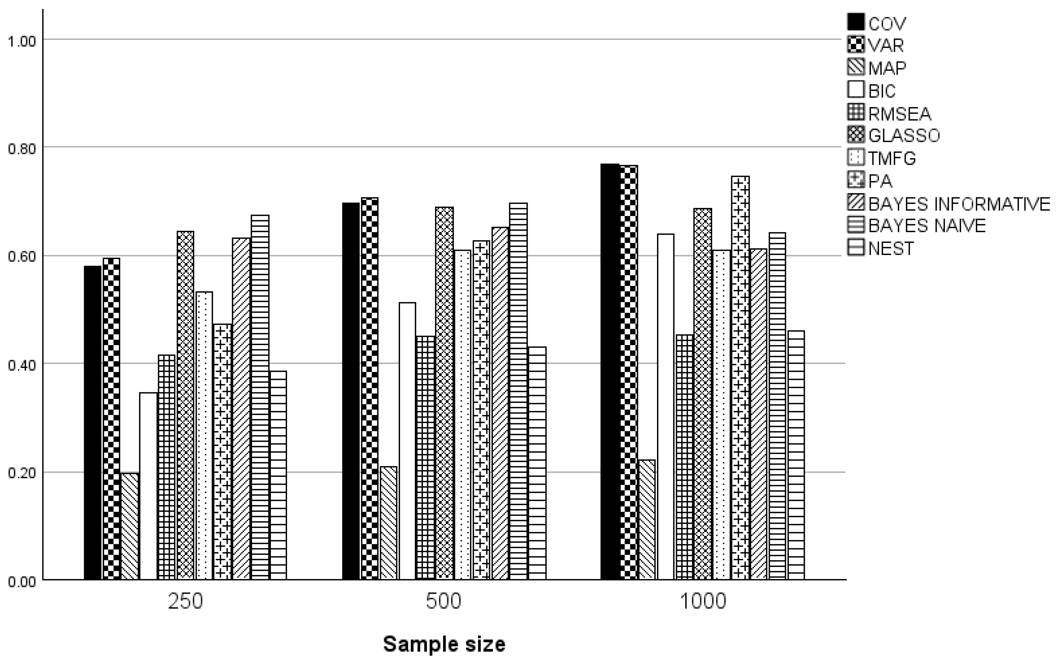
2.6. Sample Size
2.7. Methods for Determining the Number of Factors
2.8. Study Outcomes
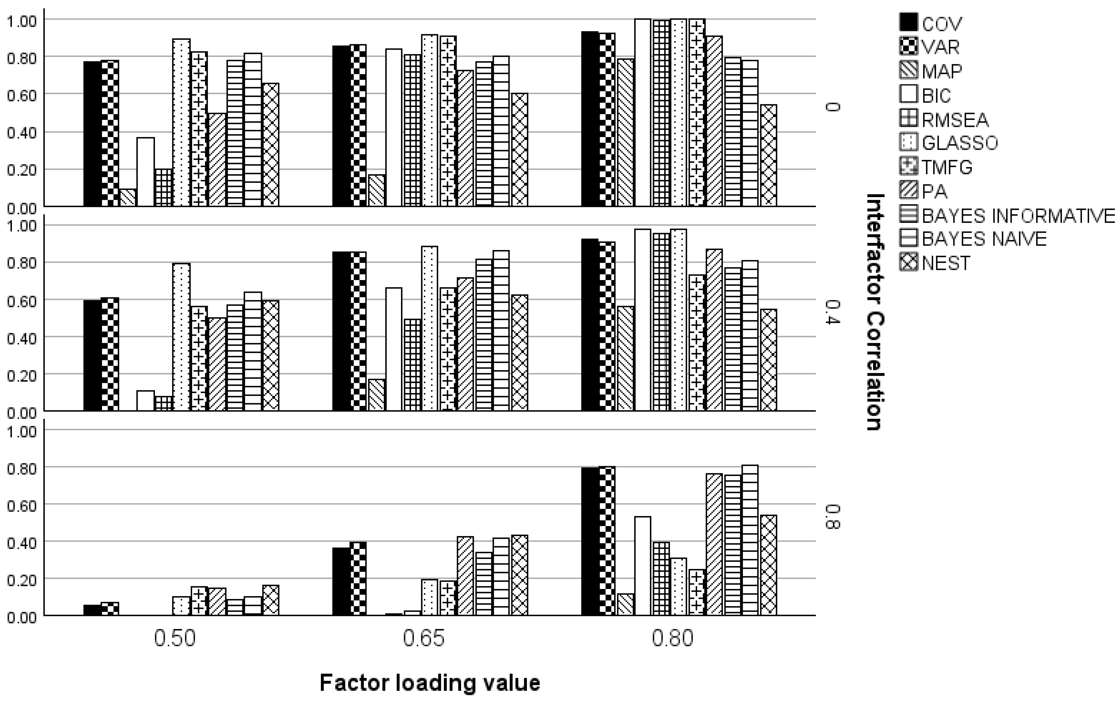
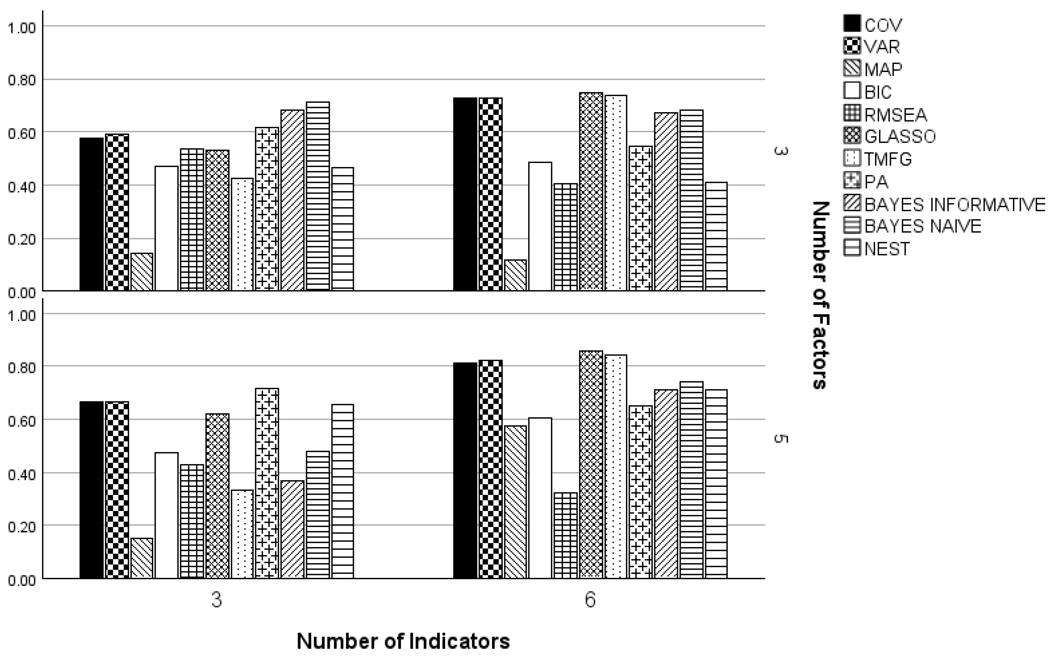
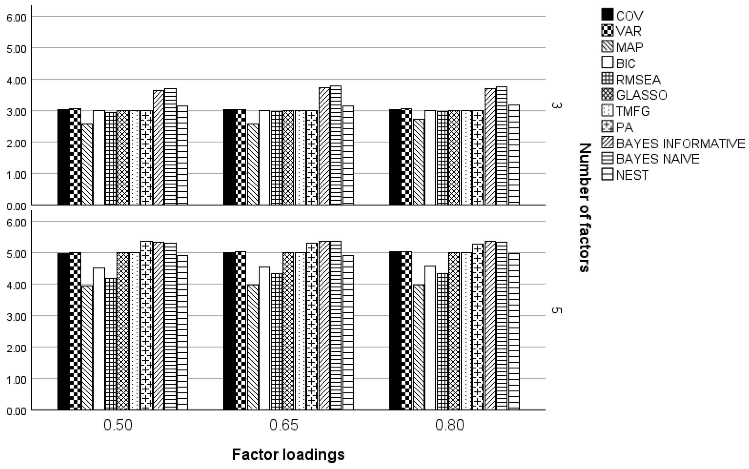
3. Results
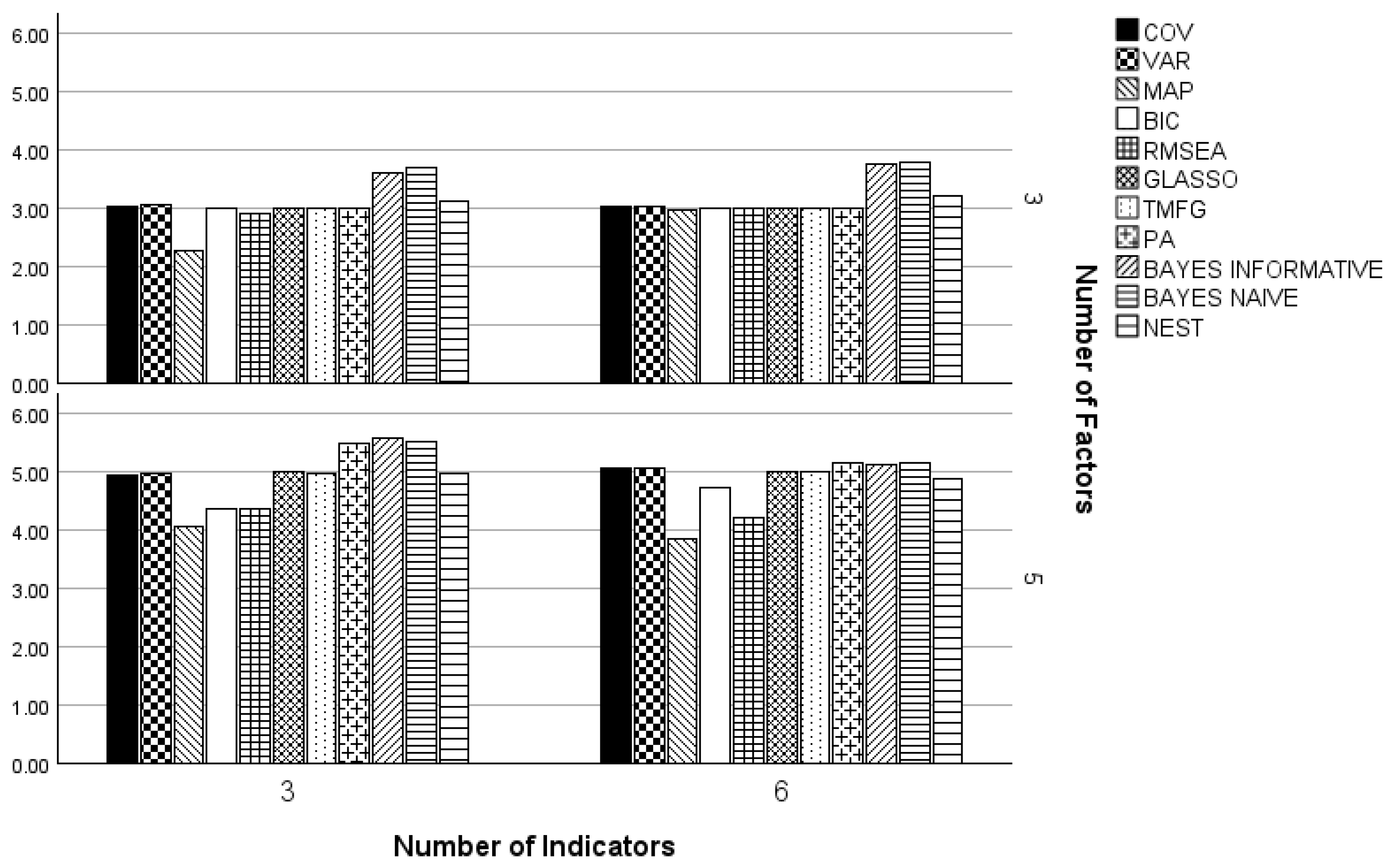
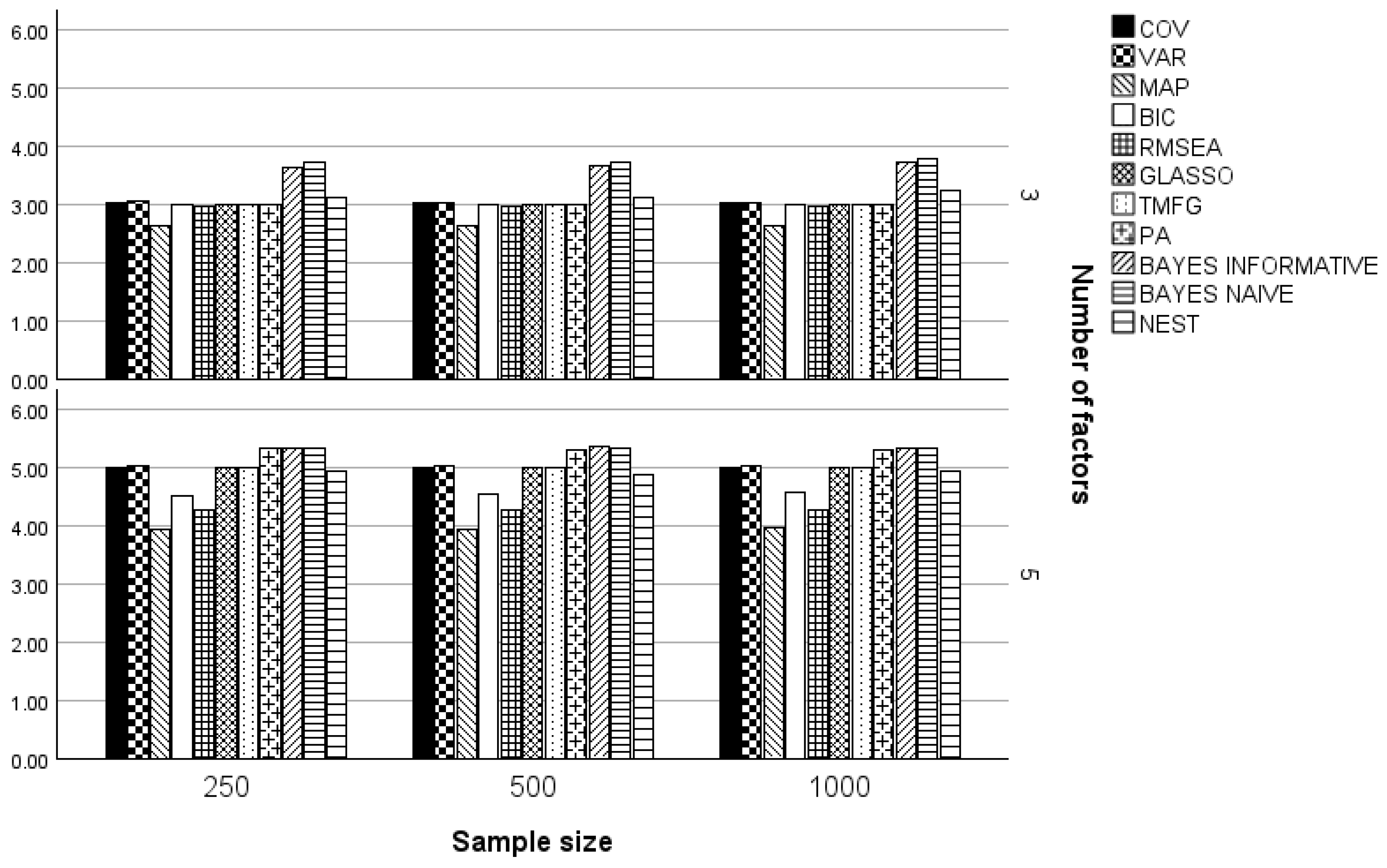
3.1. Three and Five Factors
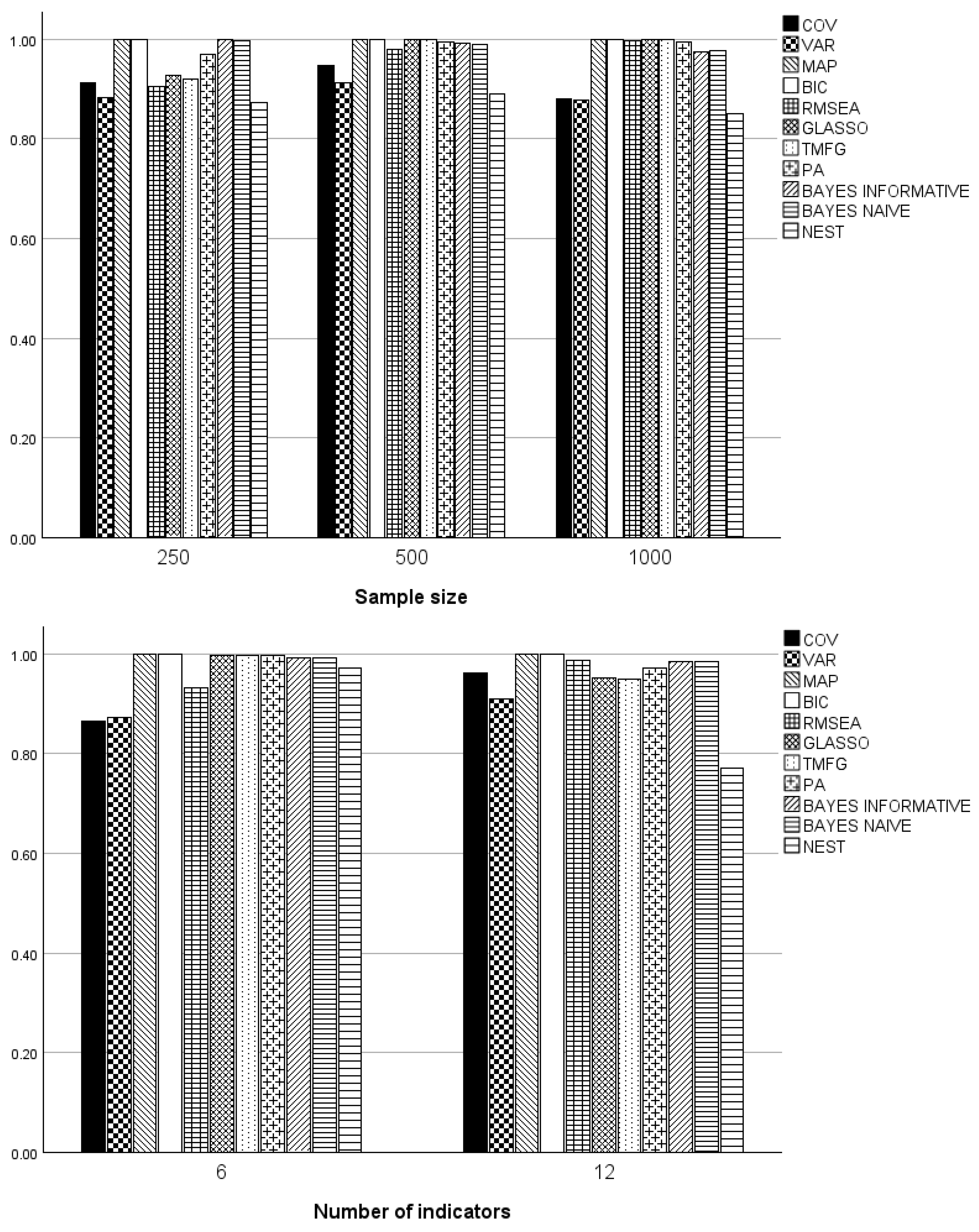
3.2. One Factor
4. Discussion
4.1. Implications for Practice
4.2. Study Limitations
5. Conclusions
Funding
Data Availability Statement
Conflicts of Interest
References
- Achim, A. (2017). Testing the number of required dimensions in exploratory factor analysis. The Quantitative Methods for Psychology, 13(1), 64–74. [Google Scholar] [CrossRef]
- Auerswald, M., & Moshagen, M. (2019). How to determine the number of factors to retain in exploratory factor analysis: A comparison of extraction methods under realistic conditions. Psychological Methods, 24(4), 468–491. [Google Scholar] [CrossRef] [PubMed]
- Barendse, M. T., Oort, F. J., & Timmerman, M. E. (2015). Using exploratory factor analysis to determine the dimensionality of discrete responses. Structural Equation Modeling, 22(1), 87–101. [Google Scholar] [CrossRef]
- Brandenburg, N., & Papenberg, M. (2024). Reassessment of innovative methods to determine the number of factors: A simulation-based comparison of exploratory graph analysis and next eigenvalue sufficiency test. Psychological Methods, 29(1), 21–47. [Google Scholar] [CrossRef] [PubMed]
- Browne, M. W., & Cudeck, R. (1989). Alternative ways of assessing model fit. Sociological Methods & Research, 21(2), 230–258. [Google Scholar]
- Canivez, G. L., Watkins, M. W., & McGill, R. J. (2019). Construct validity of the Wechsler Intelligence Scale For Children—Fifth UK Edition: Exploratory and confirmatory factor analyses of the 16 primary and secondary subtests. British Journal of Educational Psychology, 89(2), 195–224. [Google Scholar] [CrossRef]
- Caron, P.-O. (2018). Minimum average partial correlation and parallel analysis: The influence of oblique structures. Communications in Statistics–Simulation and Computation, 48(7), 2110–2117. [Google Scholar] [CrossRef]
- Clark, D. A., & Bowles, R. P. (2018). Model fit and item factor analysis: Overfactoring, underfactoring, and a program to guide interpretation. Multivariate Behavioral Research, 53(4), 544–558. [Google Scholar] [CrossRef]
- Cohen, J. (1988). Statistical power analysis for the behavioral sciences (2nd ed.). Lawrence Erlbaum Associates, Publishers. [Google Scholar]
- Coker, J. L., Catlin, D., Ray-Griffith, S., Knight, B., & Stowe, Z. N. (2018). Buprenorphine medication-assisted treatment during pregnancy: An exploratory factor analysis associated with adherence. Drug and Alcohol Dependence, 192, 146–149. [Google Scholar] [CrossRef]
- Conti, G., Fruhwirth-Schnatter, S., Heckman, J., & Piatek, R. (2014). Bayesian exploratory factor analysis. NRN working paper. In The austrian center for labor economics and the analysis of the welfare state. Johannes Kepler University. [Google Scholar]
- Epskamp, S., Rhemtulla, M., & Borsboom, D. (2017). Generalized network psychometrics: Combining network and latent variable models. Psychometrika, 82, 904–927. [Google Scholar] [CrossRef] [PubMed]
- Fabrigar, L. R., & Wegener, D. T. (2011). Exploratory factor analysis. Oxford University Press. [Google Scholar]
- Fan, J., Liao, Y., & Mincheva, M. (2013). Large Covariance Estimation by Thresholding Principal Components. Journal of the Royal Statistical Society, Series B, 75(4), 603–680. [Google Scholar] [CrossRef] [PubMed]
- Finch, W. H. (2019). Exploratory factor analysis. Sage. [Google Scholar]
- Finch, W. H. (2020). Using fit statistic differences to determine the optimal number of factors to retain in an exploratory factor analysis. Educational and Psychological Measurement, 80(2), 217–241. [Google Scholar] [CrossRef] [PubMed]
- Friedman, J., Hastie, T., & Tibshirani, R. (2008). Sparse inverse covariance estimation with the graphical lasso. Biostatistics, 9(3), 432–441. [Google Scholar] [CrossRef]
- Garrido, L. E., Abad, F. J., & Ponsoda, V. (2011). Performance of Velicer’s Minimum Average Partial Factor Retention Method with Categorical Variables. Educational and Psychological Measurement, 71(3), 551–570. [Google Scholar] [CrossRef]
- Golino, H. F., & Epskamp, S. (2017). Exploratory graph analysis: A new approach for estimating the number of dimensions in psychological research. PLoS ONE, 12(6), e0174035. [Google Scholar] [CrossRef] [PubMed]
- Golino, H., Shi, D., Christensen, A. P., Garrido, L. E., Nieto, M. D., Sadana, R., Thiyagarajan, J. A., & Martinez-Molina, A. (2020). Investigating the performance of exploratory graph analysis and traditional techniques to identify the number of latent factors: A simulation and tutorial. Psychological Methods, 25(3), 292–320. [Google Scholar] [CrossRef] [PubMed]
- Gorsuch, R. L. (1983). Factor analysis. Psychology Press. [Google Scholar]
- Haslbeck, J. M. B., & van Bork, R. (2024). Estimating the number of factors in exploratory factor analysis via out-of-sample prediction errors. Psychological Methods, 29(1), 48–64. [Google Scholar] [CrossRef] [PubMed]
- Hirose, K., & Yamamoto, M. (2015). Sparse Estimation via Nonconcave Penalized Likelihood in Factor Analysis Model. Statistical Computing, 25, 863–875. [Google Scholar] [CrossRef]
- Horn, J. L. (1965). A Rationale and Test for the Number of Factors in Factor Analysis. Psychometrika, 30(2), 179–185. [Google Scholar] [CrossRef]
- Hudson, G. (2024). EGAnet: Exploratory graph analysis. R Library. [Google Scholar]
- Kaiser, H. F. (1970). A second generation little jiffy. Psychometrika, 35, 401–415. [Google Scholar] [CrossRef]
- Kaplan, D. (2014). Bayesian statistics for the social sciences. Guilford Press. [Google Scholar]
- Liu, Y., & Zumbo, B. D. (2012). Impact of outliers arising from unintended and unknowingly included subpopulations on the decisions about the number of factors in exploratory factor analysis. Educational and Psychological Measurement, 72(3), 388–414. [Google Scholar] [CrossRef]
- Massara, G. P., Di Matteo, T., & Aste, T. (2016). Network filtering for big data: Triangulated maximally filtered graph. Journal of Complex Networks, 5, 161–178. [Google Scholar] [CrossRef]
- Orcan, F., & Imam, K. S. (2024). MonteCarloSEM. R Library. [Google Scholar]
- Patek, R. (2024). BayesFM: Bayesian inference for factor modeling. R Statistical Library. [Google Scholar]
- Pons, P., & Latapy, M. (2005). Computing Communities in Large Networks Using Random Walks. In P. Yolum, T. Güngör, F. Gürgen, & C. Özturan (Eds.), Computer and information sciences—ISCIS 2005. ISCIS 2005. lecture notes in computer science (Vol. 3733). Springer. [Google Scholar]
- Preacher, K. J., & MacCallum, R. C. (2003). Repairing Tom Swift’s Electric Factor Analysis Machine. Understanding Statistics, 2, 13–43. [Google Scholar] [CrossRef]
- Preacher, K. J., Zhang, G., Kim, C., & Mels, G. (2013). Choosing the optimal number of factors in exploratory factor analysis: A model selection perspective. Multivariate Behavioral Research, 48(1), 28–56. [Google Scholar] [CrossRef] [PubMed]
- Ratti, V., Vickerstaff, V., Crabtree, J., & Hassiotis, A. (2017). An Exploratory Factor Analysis and Construct Validity of the Resident Choice Assessment Scale with Paid Carers of Adults with Intellectual Disabilities and Challenging Behavior in Community Settings. Journal of Mental Health Research in Intellectual Disabilities, 10(3), 198–216. [Google Scholar] [CrossRef]
- R Development Team. (2024). R: A language and environment for statistical computing. R Development Team. [Google Scholar]
- Revelle, W. (2022). Psych: Procedures for psychological, psychometric, and personality research. R Library. [Google Scholar]
- Ruscio, J., & Roche, B. (2012). Determining the number of factors to retain in an exploratory factor analysis using comparison data of known factorial structure. Psychological Assessment 24, 282–292. [Google Scholar] [CrossRef]
- Shi, D., Maydeu-Olivares, A., & Rosseel, Y. (2020). Assessing fit in ordinal factor analysis models: SRMR vs RMSEA. Structural Equation Modeling: A Multidisciplinary Journal, 27(1), 1–15. [Google Scholar] [CrossRef]
- Tibshirani, R. (1996). Regression shrinkage and selection via the lasso. Journal of the Royal Statistical Society Series B. Methodological, 58, 267–288. [Google Scholar] [CrossRef]
- Velicer, W. F. (1976). Determining the Number of Components from the Matrix of Partial Correlations. Psychometrika, 41(3), 321–327. [Google Scholar] [CrossRef]
- Wirth, R. J., & Edwards, M. C. (2007). Item factor analysis: Current approaches and future directions. Psychological Methods, 12(1), 58–79. [Google Scholar] [CrossRef] [PubMed]
- Xia, Y. (2021). Determining the number of factors when population models can be closely approximated by parsimonious models. Educational and Psychological Measurement, 81(6), 1143–1171. [Google Scholar] [CrossRef] [PubMed]
- Yang, Y., & Xia, Y. (2015). On the number of factors to retain in exploratory factor analysis for ordered categorical data. Behavior Research Methods, 47(3), 756–772. [Google Scholar] [CrossRef]
- Zwick, W. R., & Velicer, W. F. (1986). Comparison of five rules for determining the number of components to retain. Psychological Bulletin, 99(3), 432–442. [Google Scholar] [CrossRef]


| Method | Determination of Number of Factors |
|---|---|
| Parallel analysis | Comparison of the observed eigenvalues with the bootstrap distribution of eigenvalues under the null of no factor structure. Retain a factor if its observed eigenvalue is greater than the 95th percentile of the null distribution. |
| Minimum average partial | Retain the number of factors corresponding to the minimum average correlation among indicators after partialing out the variance due to the factors. |
| Comparison of model fit statistics | Use the difference in the RMSEA values to determine the number of factors to retain. When the difference in the RMSEA between factor solutions exceeds 0.015, retain the model with the smaller RMSEA. |
| GLASSO | The number of factors to retain is a penalized parameter that is estimated by the model using the Walktrap algorithm. More specifically, it is the value that minimizes the penalized least squares criterion. |
| Next eigenvalue sufficiency test | A comparison of the observed eigenvalues from the principal components of the observed data with the eigenvalues for the data generated under the null hypothesis of m (e.g., 0, 1, 2…) factors. If the observed eigenvalue for m + 1 factors is greater than the 95th percentile of the eigenvalues for the m + 1 factor, given the data generated assuming a latent structure of m factors, then reject the null of m factors, and generate data assuming m + 1 factors. Continue until the null hypothesis is no longer rejected. |
| Out-of-sample prediction error | Split the sample into a training and test set. Fit an EFA model for m factors using the training set. Use the factor model obtained from the training set to predict the values of the indicators for the test set. Repeat for all the desired values of m factors and retain the number of factors that minimizes the average prediction error for the indicator variables. |
| Bayesian EFA | Fit the EFA model and estimate the number of factors to retain as a model parameter. The number of factors to retain is the median of the posterior distribution for the number of factors parameter. |
| Number of Indicators | Sample Size | ||||
|---|---|---|---|---|---|
| Method | 6 | 12 | 250 | 500 | 1000 |
| COV | 1.06 | 1.09 | 1.08 | 1.07 | 1.07 |
| VAR | 1.04 | 1.09 | 1.07 | 1.06 | 1.06 |
| MAP | 1 | 1 | 1 | 1 | 1 |
| BIC | 1 | 1 | 1 | 1 | 1 |
| RMSEA | 0.98 | 0.90 | 0.93 | 0.95 | 0.96 |
| GLASSO | 1.03 | 1.10 | 1.13 | 1.02 | 1 |
| TMFG | 1.04 | 1.12 | 1.15 | 1.03 | 1 |
| PA | 1.02 | 1.14 | 1.10 | 1.07 | 1.07 |
| Bayes-I | 1.03 | 1.07 | 1.04 | 1.05 | 1.06 |
| Bayes-N | 1.04 | 1.07 | 1.05 | 1.06 | 1.07 |
| NEST | 1.06 | 1.87 | 1.55 | 1.46 | 1.44 |
Disclaimer/Publisher’s Note: The statements, opinions and data contained in all publications are solely those of the individual author(s) and contributor(s) and not of MDPI and/or the editor(s). MDPI and/or the editor(s) disclaim responsibility for any injury to people or property resulting from any ideas, methods, instructions or products referred to in the content. |
© 2025 by the author. Licensee MDPI, Basel, Switzerland. This article is an open access article distributed under the terms and conditions of the Creative Commons Attribution (CC BY) license (https://creativecommons.org/licenses/by/4.0/).
Share and Cite
Finch, H. A Comparison of Methods for Determining the Number of Factors to Retain in Exploratory Factor Analysis for Categorical Indicator Variables. Psychol. Int. 2025, 7, 3. https://doi.org/10.3390/psycholint7010003
Finch H. A Comparison of Methods for Determining the Number of Factors to Retain in Exploratory Factor Analysis for Categorical Indicator Variables. Psychology International. 2025; 7(1):3. https://doi.org/10.3390/psycholint7010003
Chicago/Turabian StyleFinch, Holmes. 2025. "A Comparison of Methods for Determining the Number of Factors to Retain in Exploratory Factor Analysis for Categorical Indicator Variables" Psychology International 7, no. 1: 3. https://doi.org/10.3390/psycholint7010003
APA StyleFinch, H. (2025). A Comparison of Methods for Determining the Number of Factors to Retain in Exploratory Factor Analysis for Categorical Indicator Variables. Psychology International, 7(1), 3. https://doi.org/10.3390/psycholint7010003