Computable Bounds and Monte Carlo Estimates of the Expected Edit Distance ^†

Abstract

The edit distance is a metric of dissimilarity between strings, widely applied in computational biology, speech recognition, and machine learning. Let $e_k\left(n\right)$ denote the average edit distance between random, independent strings of n characters from an alphabet of size k. This paper is concerned with the efficient computation of ${\alpha }_k\left(n\right)=e_k\left(n\right)/n$ as well as of ${\alpha }_k={lim}_{n\to \infty }{\alpha }_k\left(n\right)$. It is shown that ${\alpha }_k\left(n\right)-\mathsf{\Theta }\left(\sqrt{logn/n}\right)\le {\alpha }_k\le {\alpha }_k\left(n\right)$ and that ${\alpha }_k$ is computable. An algorithm for the exact computation of ${\alpha }_k\left(n\right)$ is presented with running time $T=\mathcal{O}(n^{2}kmin(3^n,k^n))$ thus, of limited practical use. An analysis of Monte Carlo estimates, based on McDiarmid’s inequality, shows how ${\alpha }_k\left(n\right)$ can be evaluated with good accuracy and high confidence level, for rather large values of n. In particular, 99.9% confidence intervals of width approximately ${10}^{-2}$ are obtained for ${\alpha }_k$. An efficiently computable lower bound ${\beta }_k^{*}$ to ${\alpha }_k$ is derived, with ${lim}_{k\to \infty }{\beta }_k^{*}=1$. For k greater than a few dozens, significant bounds on ${\alpha }_k$ can be obtained faster via ${\beta }_k^{*}$ than by statistical methods. The above techniques yield improvements on most previous numerical estimates as well as results for alphabet sizes and string lengths not reported before.

1. Introduction

Measuring dissimilarity between strings is a fundamental problem in computer science, with applications in computational biology, speech recognition, machine learning, and other fields. One commonly used metric is the edit distance(or Levenshtein distance), defined as the minimum number of substitutions, deletions, and insertions necessary to transform one string into the other.

It is natural to ask what is the expected distance between two randomly generated strings, as the string size grows; knowledge of the asymptotic behavior has proved useful in computational biology [1] and in nearest neighbor search [2], to mention a few examples.

In computational biology, the question often arises whether two strings (e.g., two DNA reads) are noisy copies of the same source or of non-overlapping sources. In several cases of interest, the source is modeled as a sequence of independent and identically distributed symbols (see, e.g., [1,3], with reference to DNA) and the noise is modeled with substitutions, insertions, and deletions (a good approximation for technologies like PacBio and MinION [4]). Then, the statistical inference may be based on a comparison of the distance between the observed strings with either the expected distance between a string and a noisy copy of itself, or the expected distance between two random strings.

Even for uniform and independent strings, the study of the expected edit distance appears to be challenging and little work has been reported on the problem. In contrast, the closely related problem of computing the expected length of the longest common subsequence has been extensively studied, since the seminal work by Chvátal and Sankoff [5].

Using Fekete’s lemma, it can be shown that both metrics tend to grow linearly with the string size n [6]. Specifically, let $e_k\left(n\right)$ denote the expected edit distance between two random, independent strings of length n on a k-ary alphabet; then ${\alpha }_k\left(n\right)=e_k\left(n\right)/n$ approaches (from above) a limit ${\alpha }_k\in [0,1]$. Similarly, let ${\mathcal{l}}_k\left(n\right)$ denote the expected length of the longest common subsequence; then ${\gamma }_k\left(n\right)={\mathcal{l}}_k\left(n\right)/n$ approaches (from below) a limit ${\gamma }_k\in [0,1]$. The ${\gamma }_k$’s are known as the Chvátal-Sankoff constants. The efficient computation of the exact values of ${\alpha }_k$ and ${\gamma }_k$ is an open problem. This paper establishes the computability of ${\alpha }_k$, for any k, and proposes methods for estimating and bounding ${\alpha }_k$, also reporting numerical results for various alphabet sizes k.

From the perspective of computational complexity, we remark that, for the problem of computing ${\alpha }_k\left(n\right)$, given input n (for a fixed k), only algorithms that run in doubly exponential time and use exponential space are currently known, including those presented in this paper. Observe that the input size is ${log}_{2}n$, the number of bits needed to specify the problem input n. Similar statements hold for the computation of ${\gamma }_k\left(n\right)$. Therefore, at the state of the art, we can place these problems in the complexity class EXPSPACE ⊆ 2-EXPTIME, but not in EXPTIME and, a fortiori, not in PSPACE ⊆ EXPTIME. Technically, these are traditionally defined as classes of decision problems, hence our statements strictly apply to suitable decision versions of computing the constants of interest. Specifically, the decision version of computing ${\alpha }_k$ could take as inputs a (positive) integer n and an integer r such that $0\le r\le \lceil k{log}_{2}n+{log}_{2}n\rceil$ and output the r-th digit of $A_k\left(n\right)=k^{n}n{\alpha }_k\left(n\right)$. (Observe that $0\le A_k\left(n\right)\le k^{n}n$, whence $A_k\left(n\right)$ can be expresses with $\lceil n{log}_{2}k+{log}_{2}n\rceil$ bits.) Analogous considerations can be made for the problem of computing the $\nu$ most significant bits of ${\alpha }_k$ (or ${\gamma }_k$). Here, the input size is ${log}_2\nu$ and the time becomes triple exponential in the input size. Whether these problems inherently exhibit high complexity or they can be solved efficiently by exploiting a not yet uncovered deeper structure remains to be seen.

1.1. Related Work

The guaranteed, deterministic bounds presented in this paper were first published in [7]. A preliminary version of this article was published in [8] and cited in the subsequent work by Rosenfeld [9] discussed below. Details on additions and improvements of this article with respect to the conference version [7] are given in Section 1.3.

There is limited literature directly pursuing bounds and estimates for ${\alpha }_k$. It is also interesting to review results on ${\gamma }_k$: on the one hand, bounds to ${\gamma }_k$ give bounds to ${\alpha }_k$; on the other hand, techniques for analyzing ${\gamma }_k$ can be adapted for analyzing ${\alpha }_k$.

The only published estimates of ${\alpha }_k$ can be found in [1] which gives ${\alpha }_4\approx 0.518$ for the quaternary alphabet and ${\alpha }_2\approx 0.29$ for the binary alphabet. Estimates of ${\gamma }_k$ are given by Bundschuh [10], in particular ${\gamma }_2\approx 0.8126$ and ${\gamma }_4\approx 0.6544$. A similar value is reported in [11], which gives ${\gamma }_2\approx 0.8124$. Estimates of ${\gamma }_k$ by sampling are given by  [12]; their conjecture that ${\gamma }_2>0.82$ appears to be at odds with the estimate in [10]. In [13], the conjecture ${\gamma }_2\approx 0.8122$ is proposed. They also derive a closed form for the limit constant when only one string is random and the other is a periodic string containing all symbols of ${\sum }_k$.

The best published analytical lower bounds to ${\alpha }_k$ are ${\alpha }_4\ge 0.3383$ for a quaternary alphabet and ${\alpha }_2\ge 0.1578$ for a binary alphabet [1]. Recently, Rosenfeld [9] published the first systematic study of upper bounds to ${\alpha }_k$. Using an adaptation of the technique developed by Lueker for ${\gamma }_k$ [14], they established ${\alpha }_2\le 0.315514$ and ${\alpha }_4\le 0.56578$ (as well as bounds for different values of k). The best known analytical lower and upper bounds to ${\gamma }_2$ are given by [14] and improved by [15], who obtained $0.792665\le {\gamma }_2\le 0.82628$. For larger alphabets, the best lower bounds are given by  [15] and the best upper bounds are given by [11], including $0.6143\le {\gamma }_4\le 0.7082$. From known relations between the edit distance and the length of the longest common subsequence, it follows that $1-{\gamma }_k\le {\alpha }_k\le 2(1-{\gamma }_k)$. Thus, upper and lower bounds to ${\alpha }_k$ can be respectively obtained from lower and upper bounds to ${\gamma }_k$. From ${\gamma }_2\le 0.8263$ of [14], we obtain ${\alpha }_2\ge 0.1737$, which is tighter than the bound given in [1]. Instead ${\gamma }_4\le 0.7082$ of [11] yields ${\alpha }_4\ge 0.2918$, which is weaker than the bound ${\alpha }_4\ge 0.3383$ [1]. From the weaker relation $(1-{\gamma }_2)/2\le {\alpha }_2$, ref. [2] obtained the looser bound ${\alpha }_2\ge 0.0869$. In this paper, we derive improved bounds, for both ${\alpha }_2$ and ${\alpha }_4$, as well as bounds on ${\alpha }_k$, for values of k not fully addressed by earlier literature. Some of our techniques resemble those used in [16] for estimating ${\gamma }_k$.

Table 1. Comparison of lower bounds to ${\alpha }_k$ obtained in this paper and in previous work. Best known bounds are highlighted in bold face.

k	Dančík	Lueker	Ganguly et al. [1]	This Work
2	$0.162377$	$\mathbf{0.17372}$	$0.157761$	$0.170552$
3	$0.234197$	-	$0.265028$	$\mathbf{0.283660}$
4	$0.291764$	-	$0.338322$	$\mathbf{0.359783}$
5	$0.335572$	-	$0.392040$	$\mathbf{0.415173}$
6	$0.370684$	-	$0.433508$	$\mathbf{0.457766}$
7	$0.399816$	-	$0.466732$	$\mathbf{0.491836}$
8	$0.424593$	-	$0.494136$	$\mathbf{0.519901}$
16	-	-	$0.616273$	$\mathbf{0.644758}$
32	-	-	$0.708537$	$\mathbf{0.738677}$

shows lower bounds to ${\alpha }_k$ for various values of k based on this work and on that of previous authors. Lower bounds from [11,14] are obtained from upper bounds to ${\gamma }_k$, which we have translated into ${\alpha }_k\ge 1-{\gamma }_k$. Dančík reported values of the bound only for $k\le 15$. Lueker reported only the numerical upper bound to ${\gamma }_2$; his computational approach is interesting and sophisticated, but its time and space are exponential with k. Experimenting with (a minor adaptation of) the software provided by the author, we have not been able to compute ${\gamma }_3$ within reasonable time. We have obtained the values reported in the Ganguly et al. column by numerically solving their equations (in [1], only the values for $k=2$ and $k=4$ were reported). The equations underlying the results in the rightmost column of Table 1 are developed in Section 6, together with a rigorous analysis of their numerical solution.

To assess the tightness of bounds to ${\gamma }_k$, several authors have investigated the rate of convergence of ${\gamma }_k\left(n\right)$ to ${\gamma }_k$. The bound $0\le {\gamma }_k-{\gamma }_k\left(n\right)\le \mathcal{O}\left(\sqrt{logn/n}\right)$ has been obtained by [17] and, with a smaller constant, by [18]. Lueker [14] introduced a sequence of upper bounds ${\gamma }_k^h$ converging to ${\gamma }_k$ and satisfying $0\le {\gamma }_k^h-{\gamma }_k\le \mathcal{O}\left({(logh/h)}^{1/3}\right)$, where the time complexity and the space complexity of computing ${\gamma }_k^h$ increase exponentially with h. Observing that h is in turn exponential in the number $\nu$ of desired bits for ${\gamma }_k$ and that $\nu$ is exponential in the input size $\lceil {log}_2\nu \rceil$, we see that computation time is a triple exponential. No study of the rate of convergence of ${\alpha }_k\left(n\right)$ to ${\alpha }_k$ has been published. In this paper, we show that $0\le {\alpha }_k\left(n\right)-{\alpha }_k\le \mathcal{O}\left(\sqrt{logn/n}\right)$, exploiting a framework developed in [18].

Recently, Tiskin [19] has established that ${\gamma }_2$ is an algebraic number, introducing novel ideas, which may open new perspectives on the analysis of ${\gamma }_k$ and ${\alpha }_k$, for any k.

1.2. Paper Contributions and Organization

The notation and definitions used throughout this paper are given in Section 2. In Section 3, an upper bound ${\alpha }_k\left(n\right)-{\alpha }_k\le Q\left(n\right)$ is derived, for each $k\ge 2$, where $Q\left(n\right)=\mathsf{\Theta }\left(\sqrt{logn/n}\right)$ is a precisely specified function (independent of k). This implies ${\alpha }_k\in [{\alpha }_k\left(n\right)-Q\left(n\right),{\alpha }_k\left(n\right)]$, where the interval can be made arbitrarily small by choosing a suitably large n. One corollary is the computability of the real number ${\alpha }_k$, for each $k\ge 2$. Unfortunately, the algorithm underlying the computability proof is of little practical use, since the only known method to exactly compute ${\alpha }_k\left(n\right)$ is by direct application of its definition, resulting in $\mathcal{O}\left(n^2{k}^{2n}\right)$ time. Even after some improvement presented in Section 5, the upper bound ${\alpha }_k\le {\alpha }_k\left(n\right)$ is practically computable only for small values of k and n. Moreover, for the feasible values of n, $Q\left(n\right)$ is too large for the lower bound ${\alpha }_k\ge {\alpha }_k\left(n\right)-Q\left(n\right)$ to be useful. These considerations motivate the exploration of alternate approaches.

In Section 4, an analysis, based on McDiarmid’s inequality, is developed for Monte Carlo estimates of ${\alpha }_k\left(n\right)$ obtained from the edit distance of a sample of N pairs of strings. The analysis yields the radius $\Delta$ of confidence intervals for ${\alpha }_k\left(n\right)$, in terms of n, N, and the desired confidence level $\lambda$. The (sequential) time to obtain an estimate can be approximated as $T\approx {\tau }_{ed}{\displaystyle \frac{n}{{\Delta }^2}}{ln}^2\left({\displaystyle \frac{1}{1-\lambda }}\right)$, where ${\tau }_{ed}$ is of the order of 5 ns, on a typical state of the art processor core. Rather large values of n can then be dealt with. As an indication, a $\lambda =0.999$ confidence interval of radius $\Delta =0.67\times {10}^{-3}$ is obtained for ${\alpha }_k\left(2^{15}\right)$ in about 43 min. The corresponding confidence interval for ${\alpha }_k$ has radius $\Delta +{\displaystyle \frac{Q\left(2^{15}\right)}{2}}=0.00068+0.01320=0.01388$.

In Section 5, upper bounds to ${\alpha }_k$ by exact computation of ${\alpha }_k\left(n\right)$ for small values of n are obtained, by introducing an $\mathcal{O}\left(n^2{\left(3k\right)}^n\right)$ time algorithm that, while still exponential in n, is (asymptotically and practically) faster than the straightforward, $\mathcal{O}\left(n^2{\left(k^2\right)}^n\right)$ time, algorithm. When k is of the order of a few dozens, only very small values of n are feasible and ${\alpha }_k\left(n\right)$ does not differ appreciably from the quantity $1-{\displaystyle \frac{1}{k}}$, which satisfies ${\alpha }_k\left(n\right)\le 1-{\displaystyle \frac{1}{k}}$, as it can be easily shown by allowing only substitutions (cf. Hamming distance).

In Section 6, a lower bound ${\alpha }_k\ge {\beta }_k^{*}$ is established, for each $k\ge 2$. A counting argument provides a lower bound to the number of string pairs with distance at least $\beta n$; an asymptotic analysis provides conditions on $\beta$ under which the contribution to ${\alpha }_k\left(n\right)$ of the remaining string pairs vanishes with n. A careful study leads to a numerical algorithm to compute ${\beta }_k^{*}$, the supremum of the $\beta$’s satisfying such conditions, with any desired accuracy, $ϵ$. Since, as shown in Section 6, ${lim}_{k\to \infty }{\beta }_k^{*}=1$, the interval $[{\beta }_k^{*},1-{\displaystyle \frac{1}{k}}]$, which contains ${\alpha }_k$, has size vanishing with increasing k. For k large enough, it becomes a subset of a confidence interval obtained with comparable computational effort. As an example, ${\beta }_{2^{40}}^{*}\approx 0.999984\le {\alpha }_{2^{40}}\le 1-2^{-40}\approx 0.999999$, placing ${\alpha }_{2^{40}}$ in an interval of size smaller than $0.16\times {10}^{-4}$. To achieve $Q\left(n\right)\le 0.16\times {10}^{-4}$ requires $n\ge {10}^{11}$. On a single core, computing the edit distance for just one pair of strings of length $n={10}^{11}$ would take time $T\approx 5\times {10}^{-9}{10}^{22}s\approx 1.6\times {10}^6$ years, whereas computing ${\beta }_{2^{40}}^{*}$ took just 14 milliseconds, using a straightforward, non-optimized implementation.

By applying the above methodologies, we numerically derive guaranteed as well as statistical estimates for specific ${\alpha }_k$’s and ${\alpha }_k\left(n\right)$’s. In particular,

Table 2. Summary of numerical results obtained applying the methodologies presented in this paper. For various sizes k, the table shows an interval guaranteed to contain ${\alpha }_k$ and an interval containing ${\alpha }_k$ with confidence $99.9\%$. The fact that the latter is considerably narrower than the former is due to the difficulty of deriving tight guaranteed bounds.

k	Guaranteed Interval	$99.9\%$ Confidence Interval
2	$[0.17055,0.36932]$	$[0.26108,0.28884]$
3	$[0.28366,0.53426]$	$[0.40144,0.42920]$
4	$[0.35978,0.63182]$	$[0.49031,0.51807]$
5	$[0.41517,0.70197]$	$[0.55289,0.58066]$
6	$[0.45776,0.75149]$	$[0.60002,0.62778]$
7	$[0.49183,0.79031]$	$[0.63701,0.66477]$
8	$[0.51990,0.81166]$	$[0.66694,0.69470]$
16	$[0.64475,0.89554]$	$[0.79198,0.81974]$
32	$[0.73867,0.96588]$	$[0.87230,0.90007]$

summarizes our numerical results for various alphabet sizes. For each k, the table reports an interval that provably contains ${\alpha }_k$ and a (narrower) interval that contains ${\alpha }_k$ with confidence $0.999$. For the confidence interval, more details are provided in Section 4, while for the guaranteed bounds, details are given in Section 5 and Section 6.

In Section 7, we wonder about the asymptotic behavior of ${\alpha }_k$, with respect to k. We propose and motivate the conjecture that ${lim}_{k\to \infty }(1-{\alpha }_k)k=c_{\alpha }$ for some constant $c_{\alpha }\ge 1$. Numerical evidence indicates that perhaps $3\le c_{\alpha }\le 4$.

Finally, Section 8 presents conclusions and further directions of investigation.

1.3. Summary of Contributions

We now schematically summarize the key contributions of this paper. Those marked by a “*” represent novelties with respect to an earlier, conference version [7] of this work.

• (*) An analysis of the rate of convergence of ${\alpha }_k\left(n\right)$ to ${\alpha }_k$.
• (*) A proof that ${\alpha }_k$ is a computable real number.
• The coalesced dynamic programming algorithm, which can be exploited to obtain the exact value of ${\alpha }_k\left(n\right)$, unfortunately practical only for small values of n.
• (*) An analysis of the statistical estimates for ${\alpha }_k$, achieving largely improved confidence intervals (over analogous results in [7]), with a different approach based on McDiarmid’s inequality.
• A combinatorially derived lower bound on ${\alpha }_k$.
• (*) An extensive proof of correctness of the algorithm proposed to compute the lower bound on ${\alpha }_k$, with any desired precision.
• (*) A conjecture on the behavior of ${\alpha }_k$ for large k.

2. Preliminaries

In this section, we introduce the notation adopted throughout the paper and present some preliminary definitions and results used in various parts of the work.

2.1. Notation and Definitions

Let ${\sum }_k$ be a finite alphabet of size $k\ge 2$ and let $n\ge 1$ be an integer; a stringx is a sequence of symbols $x\left[1\right]x\left[2\right]\dots x\left[n\right]$ where $x\left[i\right]\in {\sum }_k$; n is called the length (or size) of x, also denoted by $\left|x\right|$. ${\sum }_k^n$ is the set of all strings of length n.

2.1.1. Edit Distance

We consider the following edit operations on a string x: the match of $x\left[i\right]$, the substitution of $x\left[i\right]$ with a different symbol $b\in {\sum }_k\setminus \left\{x\left[i\right]\right\}$, the deletion of $x\left[i\right]$, and the insertion of $b\in {\sum }_k$ in position $j=0,\dots ,n$ (insertion in j means b goes after $x\left[j\right]$ or at the beginning if $j=0$); an edit script is a sequence of edit operations. With each type of edit operation is associated a cost; throughout this paper, matches have cost 0 and other operations have cost 1. The cost of a script is the sum of the costs of its operations. The edit distance between x and y, $d_E(x,y)$, is the minimum cost of any script transforming x into y. It is easy to see that $|\left|x\right|-\left|y\right||\le d_E(x,y)\le max(\left|x\right|,\left|y\right|)$.

2.1.2. Simple Scripts

We can view a string as a sequence of cells, each containing a symbol from ${\sum }_k$, and consider edit operations as acting on such cells: a deletion destroys a cell, a substitution changes the content of a cell, and an insertion creates a new cell with some content in it (matches leave cells untouched). We will say that a script is simple if it performs at most one edit operation on each cell. It is easy to see that, if a script transforming x into y is not simple, then there is a script with fewer operations which achieves the same transformation. In fact, if a cell is eventually deleted, any operation performed on it prior to its deletion can be safely removed from the script; if a cell is inserted, any subsequent substitution can be removed, appropriately selecting the content of the initial insertion; and multiple substitutions on a cell that is retained can be either replaced by just one appropriate substitution or removed altogether. Thus, a script of minimum cost is necessarily simple, so that, to determine $d_E(x,y)$, we can restrict our attention to simple scripts.

2.1.3. Scripts and Alignments

Given an edit script transforming x into y, consider those cells of x that are retained in y, possibly with a different content. Since the relative order of two such cells is the same in x and in y, the positions occupied by such cells in x and y form an alignment, in the sense defined next.

An alignment $(\mathcal{I},\mathcal{J})$ between x and y is a pair of increasing integer sequences of the same length s

$$\begin{array}{cc}\hfill \mathcal{I}& =(i_1,\dots ,i_s)1\le i_1<i_2<\dots <i_s\le \left|x\right|,\hfill \\ \hfill \mathcal{J}& =(j_1,\dots ,j_s)1\le j_1<j_2<\dots <j_s\le \left|y\right|.\hfill \end{array}$$

The positions $i_{\mathcal{l}}$ in x and $j_{\mathcal{l}}$ in y are said to be to be aligned in $(\mathcal{I},\mathcal{J})$. To each script $\mathcal{S}$, there corresponds a unique alignment $a\left(\mathcal{S}\right)=(\mathcal{I},\mathcal{J})$, where s equals the number of cells of x that are retained in y and, for every $\mathcal{l}=1,2,\dots ,s$, the cell in position $i_{\mathcal{l}}$ of x has moved to position $j_{\mathcal{l}}$ of y. If $\mathcal{S}$ is simple, then: (i) for aligned positions $i_{\mathcal{l}}$ and $j_{\mathcal{l}}$, $y\left[j_{\mathcal{l}}\right]$ is substituted with or matched to $x\left[i_{\mathcal{l}}\right]$ depending on whether $y\left[j_{\mathcal{l}}\right]\ne x\left[i_{\mathcal{l}}\right]$ or not; (ii) for positions $i\notin \mathcal{I}$, $x\left[i\right]$ is deleted, and (iii) for positions $j\notin \mathcal{J}$, $y\left[j\right]$ is inserted.

Next, we prove a simple lemma, which will be useful both in Section 3, to cast edit distance within the framework of [18], and in Section 6, to develop a counting argument leading to a lower bound on ${\alpha }_k$.

Lemma 1. 

With the preceding notation, if $\mathcal{S}$ is a simple script to transform x into y, with $\left|x\right|=\left|y\right|=n$, and $(\mathcal{I},\mathcal{J})=a\left(\mathcal{S}\right)$ is the corresponding alignment, its cost is

$$cost(x,y,\mathcal{S})=2(n-s)+{\displaystyle \sum _{\mathcal{l}=1}^s}(x\left[i_{\mathcal{l}}\right]\ne y\left[j_{\mathcal{l}}\right]).$$

(1)

Proof. 

The script performs $(n-s)$ deletions, $(n-s)$ insertions, and ${\sum }_{\mathcal{l}=1}^s(x\left[i_{\mathcal{l}}\right]\ne y\left[j_{\mathcal{l}}\right])$ substitutions. □

We may observe that (for given x and y) simple scripts corresponding to the same alignment differ only with respect to the order in which the edit operations are applied. Such an order does not affect the final result, since in a simple script different operations act on different cells. Thus, the number of distinct simple scripts with the same alignment is the factorial of their cost (i.e., of the number of edit operations), given by Equation (1).

2.1.4. Random Strings and the Limit Constant

A random string of length n, $X=X\left[1\right]X\left[2\right]\dots X\left[n\right]$, is a sequence of random symbols $X\left[i\right]$ generated according to some distribution over ${\sum }_k$. We will assume that the $X\left[i\right]$’s are uniformly and independently sampled from ${\sum }_k$ or, equivalently, that $Pr[X=x]=k^{-n}$ for every $x\in {\sum }_k^n$. We define the eccentricity$ecc\left(x\right)$ of a string x as its expected distance from a random string $Y\in {\sum }_k^n$:

$$\begin{array}{c}\hfill ecc\left(x\right)=k^{-n}\sum _{y\in {\sum }_k^n}{d}_E(x,y).\end{array}$$

(2)

The expected edit distance between two random, independent strings of ${\sum }_k^n$ is:

$$\begin{array}{cc}\hfill e_k\left(n\right)& =k^{-2n}\sum _{x\in {\sum }_k^n}\sum _{y\in {\sum }_k^n}{d}_E(x,y)\hfill \\ \hfill & =k^{-n}\sum _{x\in {\sum }_k^n}ecc\left(x\right).\hfill \end{array}$$

(3)

Let ${\alpha }_k\left(n\right)=e_k\left(n\right)/n$; it can be shown (Fekete’s lemma from ergodic theory; see, e.g., Lemma 1.2.1 in [6]) that there exists a real number ${\alpha }_k\in [0,1]$, such that

$$\begin{array}{c}\hfill \underset{n\to \infty }{lim}{\alpha }_k\left(n\right)={\alpha }_k.\end{array}$$

(4)

The main objective of this paper is to derive estimates and bounds to ${\alpha }_k$.

2.1.5. Rate of Convergence to the Limit Constant

In the outlined context, it is of interest to develop upper bounds, as  functions of n, to the quantity

$$\begin{array}{c}\hfill q_k\left(n\right)={\alpha }_k\left(n\right)-{\alpha }_k,\end{array}$$

which we will refer to as the rate of convergence, following a terminology widely used for analogous quantities in the context of the longest common subsequence (e.g., [17,18]).

2.2. Computing the Edit Distance

The edit distance and the length of the longest common subsequence (LCS) can be computed by a dynamic programming algorithm. Given two strings, x of length n and y of length m, their edit distance $d_E(x,y)$ is obtained as the entry $M_{n,m}$ of an $(n+1)\times (m+1)$ matrix $\mathbf{M}$, computed according to the following recurrence:

$$\begin{array}{ccc}\hfill & M_{i,0}=i\hfill & \hfill \mathrm{for}i=0,\dots ,n\\ \hfill & M_{0,j}=j\hfill & \hfill \mathrm{for}j=0,\dots ,m\\ \hfill & M_{i,j}=min(M_{i-1,j-1}+{\xi }_{i,j},M_{i-1,j}+1,M_{i,j-1}+1)\hfill & \hfill \mathrm{for}i>0\mathrm{and}j>0\end{array}$$

(5)

where ${\xi }_{i,j}=0$ if $x\left[i\right]=y\left[j\right]$ and ${\xi }_{i,j}=1$ otherwise. (A similar algorithm computes the length of the LCS. Recurrence (5) becomes $M_{i,0}=0$, $M_{0,j}=0$, and $M_{i,j}=max(M_{i-1,j-1}+(1-{\xi }_{i,j}),M_{i-1,j},M_{i,j-1}).$) This algorithm takes $\mathcal{O}\left(nm\right)$ time and space. An edit script transforming x into y can be obtained backtracking on $\mathbf{M}$, along a path from cell $(n,m)$ to cell $(0,0)$. For both edit distance and LCS, the approach by [20], exploiting the method of the Four Russians, reduces the time to $\mathcal{O}\left({\displaystyle \frac{n^2}{logn}}\right)$, assuming $n\ge m$. Although asymptotically faster, the algorithm in [20] is seldomly used. Other approaches are usually preferred, such as the one proposed by [21], which reduces the $n^2$ bound by a factor proportional to the machine word size, implementing Recurrence (5) via bit-wise operations.

The space complexity of the basic dynamic programming algorithm can be reduced to $\mathcal{O}(min(n,m\left)\right)$. Assuming, w.l.o.g., that $n\ge m$, simply proceed row-wise storing only the last complete row. While this approach is not directly amenable to constructing scripts by backtracking, a more sophisticated divide and conquer version due to Hirschberg [22] yields the edit distance and an edit script in quadratic time and linear space. In [23], authors applied the Four Russians method to Hirschberg’s algorithm, improving its running time by a logarithmic factor.

It is known that both the edit distance and the length of the LCS cannot be computed in time $\mathcal{O}\left(n^{2-ϵ}\right)$, unless the Strong Exponential Time Hypothesis (SETH) is false ([24,25]).

Approximate computation of the edit distance has been extensively studied. Ukkonen [26] presents a banded algorithm that computes an approximation within a factor $\mathcal{O}\left(n^{1-ϵ}\right)$ in time $\mathcal{O}\left(n^{1+ϵ}\right)$. Interestingly, this algorithm computes the exact distance whenever such distance is $\mathcal{O}\left(n^{ϵ}\right)$ (although, it may output the exact distance also for higher values). In [27] authors give an algorithm that computes the exact distance in time $\mathcal{O}(n+d^2)$, where d is the distance itself. Thus, sub-quadratic time can be achieved when the distance is sub-linear. More recently, an ${(logn)}^{\mathcal{O}(1/ϵ)}$ approximation, computable in time $\mathcal{O}\left(n^{1+ϵ}\right)$, was proposed by  [28], and a constant approximation algorithm with running time $\mathcal{O}\left(n^{1+5/7}\right)$ was proposed by  [29,30]. The work by [31] gives a reduction from approximate length of the longest common subsequence to approximate edit distance, proving that the algorithm in [29] can also be used to approximate the length of the LCS.

In order to compute upper bounds to ${\alpha }_k$, we propose an algorithm related to the approaches developed by [14,32]. In these works, portions of the dynamic programming matrix are associated to the states of a finite state machine. Our algorithm conceptually simulates all possible executions of a machine similar to the one defined in [32].

3. Rate of Convergence and Computability of ${\mathit{\alpha }}_{\mathit{k}}$

For each n, ${\alpha }_k\left(n\right)$ is a rational number, which can be computed, according to Equation (3), by exhaustively enumerating all pairs $(x,y)$ of strings in ${\sum }_k^n$ and accumulating the corresponding values $d_E(x,y)$, which can be obtained with any algorithm for the exact edit distance. On the other hand, the limit constant ${\alpha }_k$ is known to exist as a real number, whose rationality remains an open problem. In this section, we show that, for every k, this number is computable, according to the following (standard) definition.

Definition 1  (Computability of a real number). 

A real number ζ is computable if there exists an algorithm that, given as input a rational number $ϵ>0$, outputs a rational number ${\zeta }_{ϵ}$, such that $|\zeta -{\zeta }_{ϵ}|<ϵ$.

As shown in [33], the subadditivity of a sequence of rational numbers, while sufficient to guarantee the existence of a limit (Fekete’s Lemma, [34]), is not sufficient to guarantee its computability which, if present, requires an additional argument. For ${\alpha }_k$, such an argument can be provided along the following steps:

• Prove that, for some computable function $b_k\left(n\right)$, we have

  $$\begin{array}{c}\hfill {\alpha }_k\left(n\right)-{\alpha }_k\le b_k\left(n\right)\forall n\ge 1.\end{array}$$

  (6)
• Show that there is an algorithm which, given a rational number $ϵ>0$, computes an integer $n_{ϵ}\ge 1$ such that

  $$\begin{array}{c}\hfill b_k\left(n\right)<ϵ\forall n\ge n_{ϵ}.\end{array}$$

  (7)
• Let ${\alpha }_{k,ϵ}={\alpha }_k\left(n_{ϵ}\right)$ and observe that

  $$\begin{array}{c}\hfill 0<{\alpha }_{k,ϵ}-{\alpha }_k<b_k\left(n_{ϵ}\right)<ϵ,\end{array}$$

  (8)

  thus complying with Definition 1 (with $\zeta ={\alpha }_k$ and ${\zeta }_{ϵ}={\alpha }_{k,ϵ}$), since $n_{ϵ}$ is computable from $ϵ$ and ${\alpha }_{k,ϵ}={\alpha }_k\left(n_{ϵ}\right)$ is computable from $n_{ϵ}$.

To obtain a bound $b_k\left(n\right)$ such that Equation (6) is satisfied, we show how the edit distance problem can be cast within a framework developed in [18], to analyze the limit average behavior of certain functions of random string pairs on a finite alphabet $\sum$. These functions are formally defined next.

Definition 2. 

Let $S:\sum \times \sum \to R_0^{+}$ be a symmetric ($S(b,a)=S(a,b)$), non-negative, real function and let δ be a real number. The score of a pair of strings $x,y\in {\sum }^n$, with respect to a given alignment $(\mathcal{I},\mathcal{J})$, is defined as

$$\begin{array}{c}\hfill S(x,y;\mathcal{I},\mathcal{J})={\displaystyle \sum _{\mathcal{l}=1}^s}S(x\left[i_{\mathcal{l}}\right],y\left[j_{\mathcal{l}}\right])+\delta (n-s).\end{array}$$

The score of the string pair is the maximum score over all possible alignments:

$$\begin{array}{c}\hfill S(x,y)=\underset{(\mathcal{I},\mathcal{J})}{max}S(x,y;\mathcal{I},\mathcal{J}).\end{array}$$

Next, we express the edit distance in terms of a suitable score.

Proposition 1.

For $a,b\in {\sum }_k$ let

$$\begin{array}{c}\hfill S(a,b)=\left\{\begin{array}{cc}0\hfill & ifa\ne b\hfill \\ 1\hfill & \mathit{otherwise}\hfill \end{array}\right.\end{array}$$

and let $\delta =-1$. Then, for $x,y\in {\sum }_k^n$,

$$\begin{array}{c}\hfill d_E(x,y)=n-S(x,y).\end{array}$$

(9)

Proof. 

Considering a given alignment $(\mathcal{I},\mathcal{J})$, we can write

$$\begin{array}{cc}\hfill n-S(x,y;\mathcal{I},\mathcal{J})& =n-{\displaystyle \sum _{\mathcal{l}=1}^s}S(x\left[i_{\mathcal{l}}\right],y\left[j_{\mathcal{l}}\right])-(-1)(n-s)\hfill \\ \hfill & =2(n-s)+\left(s-{\displaystyle \sum _{\mathcal{l}=1}^s}S(x\left[i_{\mathcal{l}}\right],y\left[j_{\mathcal{l}}\right])\right)\hfill \\ \hfill & =2(n-s)+{\displaystyle \sum _{\mathcal{l}=1}^s}(x\left[i_{\mathcal{l}}\right]\ne y\left[j_{\mathcal{l}}\right]).\hfill \end{array}$$

Recalling Lemma 1, the quantity in the last row can be recognized as the cost of the simple scripts $\mathcal{S}$ transforming x into y, with alignment $a\left(\mathcal{S}\right)=(\mathcal{I},\mathcal{J})$. Further recalling that optimal scripts are simple, we conclude that maximizing the score with respect to the alignment minimizes the cost of the edit script, whence the claimed Equality (9). □

The preceding proposition enables the application of the following far reaching result to the analysis of the average edit distance.

Theorem 1

([18]). Let X and Y be random strings in ${\sum }^n$, whose symbols are all mutually independent and equally distributed. Let $l\left(n\right)={\displaystyle \frac{1}{n}}{E}_{X,Y}S(X,Y)$, where E denotes the expectation operator, and let $l={lim}_{n\to \infty }l\left(n\right)$. Then

$$\begin{array}{c}\hfill l-l\left(n\right)\le A\sqrt{{\displaystyle \frac{2}{n-1}}\left({\displaystyle \frac{n+1}{n-1}}+ln(n-1)\right)}+{\displaystyle \frac{F}{n-1}}:=Q_{A,F}\left(n\right).\end{array}$$

(10)

where $A={max}_{a,b\in \sum }S(a,b)$ and $F={max}_{a,b,c\in \sum }|S(a,b)-S(a,c)|$.

The preceding theorem makes no assumption on the probability distribution of the symbols. Moreover, $Q_{A,F}\left(n\right)$ is independent of such distribution, although the quantities $l\left(n\right)$ and l are not. Here, we assume the uniform distribution, upon which we have based the definition of ${\alpha }_k\left(n\right)$. As a corollary of Theorem 1 and Proposition 1, we obtain the computability of ${\alpha }_k$.

Theorem 2.

For any integer $k>0$, the limit constant ${\alpha }_k$ defined in Equation (4) satisfies the bound

$$\begin{array}{c}\hfill {\alpha }_k\left(n\right)-{\alpha }_k\le \sqrt{{\displaystyle \frac{2}{n-1}}\left({\displaystyle \frac{n+1}{n-1}}+ln(n-1)\right)}+{\displaystyle \frac{1}{n-1}}:=Q\left(n\right),\end{array}$$

(11)

for $n\ge 2$. Therefore, ${\alpha }_k$ is a computable real number.

Proof. 

It is an exercise to see that, for the score function $S(a,b)$ of Proposition 1, $A=F=1$, for any k. Correspondingly, we have $Q\left(n\right)=Q_{1,1}\left(n\right)$. We also observe that, with $\sum ={\sum }_k$, using Equation (9), we have

$$\begin{array}{cc}\hfill {\alpha }_k\left(n\right)& ={\displaystyle \frac{1}{n}}{E}_{X,Y}{d}_E(X,Y)=1-{\displaystyle \frac{1}{n}}{E}_{X,Y}S(X,Y)=1-l_k\left(n\right)\hfill \\ \hfill {\alpha }_k& =1-l_k.\hfill \end{array}$$

Thus, Equation (11) follows from Equation (10), with $Q\left(n\right)=Q_{1,1}\left(n\right)$, considering that ${\alpha }_k\left(n\right)-{\alpha }_k=(1-l_k\left(n\right))-(1-l_k)=l_k-l_k\left(n\right)$. Finally, it is straightforward to prove that there is an integer $\overline{n}$ such that $Q\left(n\right)$ is strictly decreasing for $n\ge \overline{n}$ and that $n_{ϵ}=min\{n\ge \overline{n}:Q\left(n\right)<ϵ\}$ is a computable function of the rational number $ϵ$. □

Interestingly, $Q\left(n\right)$, hence $n_{ϵ}$, is independent both of the alphabet size, k, and of the probabilities of symbols in the alphabet $\sum$. However, computing ${\alpha }_k\left(n_{ϵ}\right)$, to obtain a deterministically guaranteed $ϵ$-approximation of ${\alpha }_k$, will require work increasing with k, at least with the currently known approaches that are sensitive to the number $k^n$ of strings of length n, as we will see in the coming sections. Moreover, $n_{ϵ}$ increases more than quadratically with $1/ϵ$ (see Equation (11)), making the approach completely impractical. More specifically, to obtain $\nu$ bits of ${\alpha }_k$ we need $ϵ=2^{-\nu }$, so that $n_{ϵ}\ge 1/{ϵ}^2=4^{\nu }$ and $k^{n_{ϵ}}\ge k^{4^{\nu }}$, which is a triple exponential in the problem size ${log}_2\nu$.

Remark 1.

Although, both for simplicity and for homogeneity with other sections, we have stated Theorem 2 for the case of uniform distribution on the alphabet symbols, the arguments that have been developed are easily adapted to establish the computability for the analog of ${\alpha }_k$, under any distribution. In fact, as already observed, $Q_{A,F}\left(n\right)$ is independent of the distribution and the quantities analog to the $l\left(n\right)$’s are trivially (although inefficiently) computable by summing the distances $d_E(x,y)$ over all pairs $x,y\in {\sum }_k^n$, duly weighted by their probabilities.

We point out that, in the same spirit of this section, the computability of ${\gamma }_k$ can be derived from any of the rate-of-convergence bounds given by [14,17,18].

4. Monte Carlo Estimates of ${\mathit{\alpha }}_{\mathit{k}}$

In this section, motivated by the difficulty of the exact computation, we develop an analysis of Monte Carlo estimates of ${\alpha }_k\left(n\right)$, by sampling, and translate them into estimates of ${\alpha }_k$, using Theorem 2. We will see how ${\alpha }_k\left(n\right)$ can be estimated with high confidence and good accuracy for values of n up to a quarter million, with less than one core-hour of computation. For ${\alpha }_k$, we achieve an error of the order of ${10}^{-2}$.

Intuitively, for fixed k and n, we expect the estimate error to be proportional to $1/\sqrt{N}$, where N is the number of samples (string pairs), and to the standard deviation $S_k\left(n\right)/n$ of the single sample $d_E(x,y)/n$. Experimentally, this standard deviation appears to decrease a bit faster than $1/\sqrt{n}$, (We do not report here on this experimental observation systematically; however, estimates of $S_4\left(n\right)$ for some values of n can be found in

Table 3. Estimates ${\tilde{e}}_4(n,N)$ of the average edit distance and ${\tilde{\alpha }}_4(n,N)={\displaystyle \frac{1}{n}}{\tilde{e}}_4(n,N)$ of the average distance per symbol ${\alpha }_4\left(n\right)$, for various string lengths n, based on $N=2^{39}/n^2$ samples. The last column shows the confidence intervals for ${\alpha }_4\left(n\right)$ corresponding to confidence level $99.9\%$. ${\tilde{S}}_4(n,N)$ is the sample standard deviation of the single-pair distance.

n	N	${\mathbf{\Delta }}_{99.9\%}(\mathit{n},\mathit{N})$	${\tilde{\mathit{e}}}_4(\mathit{n},\mathit{N})$	${\tilde{\mathit{S}}}_4(\mathit{n},\mathit{N})$	${\tilde{\mathit{\alpha }}}_4(\mathit{n},\mathit{N})$	$99.9\%$ Conf. Int.
$2^8$	$2^{23}$	$0.59\times {10}^{-4}$	$138.10$	$3.838$	$0.53946$	$[0.53940,0.53953]$
$2^9$	$2^{21}$	$0.84\times {10}^{-4}$	$272.10$	$4.920$	$0.53144$	$[0.53135,0.53153]$
$2^{10}$	$2^{19}$	$0.12\times {10}^{-3}$	$538.77$	$6.307$	$0.52614$	$[0.52602,0.52626]$
$2^{11}$	$2^{17}$	$0.17\times {10}^{-3}$	$1070.4$	$8.146$	$0.52263$	$[0.52246,0.52280]$
$2^{12}$	$2^{15}$	$0.24\times {10}^{-3}$	$2131.5$	$10.56$	$0.52039$	$[0.52015,0.52063]$
$2^{13}$	$2^{13}$	$0.34\times {10}^{-3}$	$4250.9$	$13.62$	$0.51891$	$[0.51857,0.51925]$
$2^{14}$	$2^{11}$	$0.48\times {10}^{-3}$	$8487.0$	$17.71$	$0.51801$	$[0.51753,0.51849]$
$2^{15}$	$2^9$	$0.67\times {10}^{-3}$	16,954	$24.98$	$0.51739$	$[0.51671,0.51807]$
$2^{16}$	$2^7$	$0.95\times {10}^{-3}$	33,884	$29.12$	$0.51704$	$[0.51608,0.51799]$
$2^{17}$	$2^5$	$0.13\times {10}^{-2}$	67,734	$38.85$	$0.51677$	$[0.51542,0.51812]$
$2^{18}$	$2^3$	$0.19\times {10}^{-2}$	135,450	$62.94$	$0.51670$	$[0.51479,0.51861]$

) with the implication that, to obtain the same error on ${\alpha }_k\left(n\right)$, fewer samples suffice for larger n. However, the behavior of the standard deviation does not appear easy to establish analytically. Fortunately, the edit distance function has the property that, if only one position is modified in just one of the input strings, the (absolute value of the) variation of the distance is at most 1. This property enables the use of McDiarmid’s inequality to bound from above the probability that $d_E(x,y)/n$ deviates from the mean by more than a certain amount, by a negative exponential in the square of that amount. This paves the way to the desired analysis. In fact, McDiarmid’s inequality can be applied directly to the average over N samples, dealing in a uniform way with the “averaging” effect within a single pair of strings and across multiple pairs.

• Preview of results

To help navigate this section, we preview its results, with a preliminary interpretation.

In Section 4.1, we present Monte Carlo estimates of ${\alpha }_k\left(n\right)$ for which we develop confidence intervals based on McDiarmid’s inequality. The results for the quaternary alphabet (column ${\tilde{\alpha }}_4(n,N)$ of Table 3) show that these values converge from above to ${\alpha }_k$. We observe that the differences ${\tilde{\alpha }}_4(n,N)-{\tilde{\alpha }}_4(2n,N)$ decrease with n, suggesting that the estimates become more precise as n increases, even if the confidence intervals become wider, due to the smaller sample size N, manageable within a given computational budget. The dependence of ${\alpha }_k\left(n\right)$ upon k is investigated

Table 4. Estimates ${\tilde{e}}_k(n,N)$ of the average edit distance and ${\tilde{\alpha }}_k(n,N)={\displaystyle \frac{1}{n}}{\tilde{e}}_k(n,N)$ of the average distance per symbol ${\alpha }_k\left(n\right)$, for various alphabet sizes k, based on $N=2^9$ samples of pairs of strings with length $n=2^{15}$. The confidence radius is ${\Delta }_{99.9\%}(n,N)={\Delta }_{99.9\%}(2^{15},2^9)\approx 0.67\times {10}^{-3}$; the corresponding confidence intervals for ${\alpha }_k\left(n\right)$ are given in the last column. ${\tilde{S}}_k(n,N)$ is the sample standard deviation of the single-pair distance.

k	${\tilde{\mathit{e}}}_{\mathit{k}}(\mathit{n},\mathit{N})$	${\tilde{\mathit{S}}}_{\mathit{k}}(\mathit{n},\mathit{N})$	${\tilde{\mathit{\alpha }}}_{\mathit{k}}(\mathit{n},\mathit{N})$	$99.9\%$ Conf. Int.
2	$9442.6$	$26.04$	$0.28817$	$[0.28749,0.28884]$
3	14,042	$24.88$	$0.42852$	$[0.42784,0.42920]$
4	16,954	$24.98$	$0.51739$	$[0.51671,0.51807]$
5	19,005	$22.78$	$0.57998$	$[0.57930,0.58066]$
6	20,549	$22.00$	$0.62710$	$[0.62642,0.62778]$
7	21,761	$21.05$	$0.66409$	$[0.66341,0.66477]$
8	22,742	$20.15$	$0.69402$	$[0.69334,0.69470]$
16	26,839	$16.38$	$0.81906$	$[0.81838,0.81974]$
32	29,471	$14.10$	$0.89939$	$[0.89871,0.90007]$

. Here, all confidence intervals have the same width, since the same values of n and N are used for different k’s.

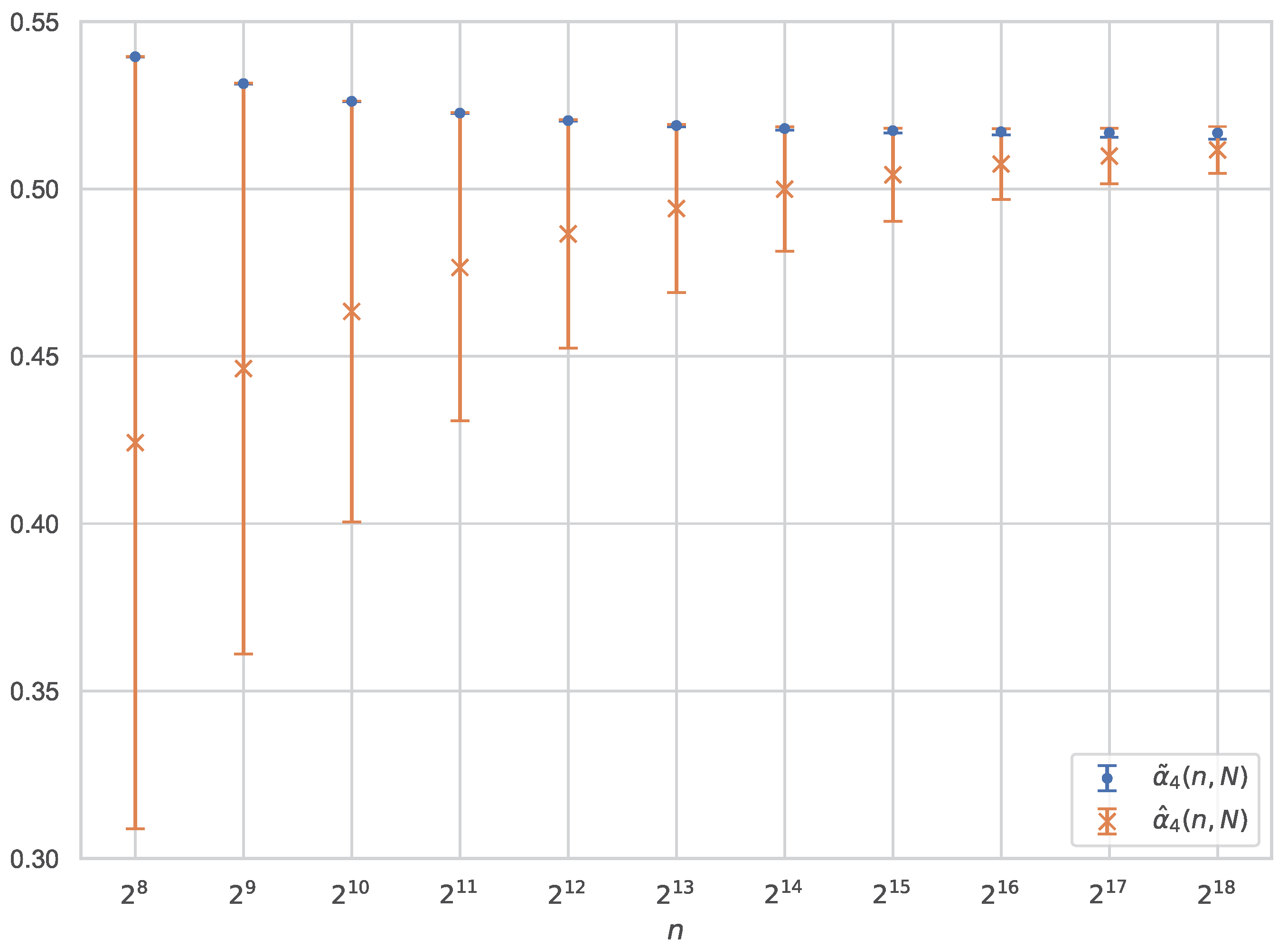
In Section 4.2, we derive estimates of ${\alpha }_k$ (the limit of ${\alpha }_k\left(n\right)$) and corresponding confidence intervals. These estimates for $k=4$ (column ${\widehat{\alpha }}_k(n,N)$ in

Table 5. Estimates ${\widehat{\alpha }}_4(n,N)$ of ${\alpha }_4$ with confidence intervals for various string lengths n, based on $N=2^{39}/n^2$ samples (so that each estimate takes approximately the same computation time). $I_4(n,N,\Delta )$ is the corresponding $99.9\%$ confidence interval for ${\alpha }_4$. The estimates improve with growing n, as witnessed by the decrease of the interval radius $R_{0.999}(n,N)$.

n	N	${\mathit{R}}_{0.999}(\mathit{n},\mathit{N})$	${\widehat{\mathit{\alpha }}}_4(\mathit{n},\mathit{N})$	${\mathit{I}}_4(\mathit{n},\mathit{N},\mathbf{\Delta })$
$2^8$	$2^{23}$	$0.11534$	$0.42418$	$[0.30884,0.53953]$
$2^9$	$2^{21}$	$0.08523$	$0.44629$	$[0.36105,0.53153]$
$2^{10}$	$2^{19}$	$0.06287$	$0.46338$	$[0.40051,0.52626]$
$2^{11}$	$2^{17}$	$0.04631$	$0.47649$	$[0.43075,0.52280]$
$2^{12}$	$2^{15}$	$0.03409$	$0.48654$	$[0.45244,0.52063]$
$2^{13}$	$2^{13}$	$0.02512$	$0.49413$	$[0.46900,0.51925]$
$2^{14}$	$2^{11}$	$0.01858$	$0.49990$	$[0.48132,0.51849]$
$2^{15}$	$2^9$	$0.01388$	$0.50419$	$[0.49031,0.51807]$
$2^{16}$	$2^7$	$0.01056$	$0.50742$	$[0.49685,0.51799]$
$2^{17}$	$2^5$	$0.00833$	$0.50979$	$[0.50145,0.51812]$
$2^{18}$	$2^3$	$0.00698$	$0.51163$	$[0.50465,0.51861]$

) are obtained as the center point of a confidence interval depending on both statistical interval and the bound $Q\left(n\right)$ on ${\alpha }_k\left(n\right)-{\alpha }_k$. Interestingly, the width of such interval is largely due to $Q\left(n\right)$. Furthermore, the bound appears to be loose, since the values ${\widehat{\alpha }}_k(n,N)$ converge to ${\alpha }_k$ from below, whereas the ${\tilde{\alpha }}_k(n,N)$ converge from above.

Table 6. Estimates of ${\alpha }_k$ for various alphabet sizes k, based on $N=2^9$ samples of pairs of string with length $n=2^{15}$. The radius of the interval $I_k(n,N,\Delta )$ is based on a $\lambda =0.999$ confidence level and is $R_{0.999}(2^{15},2^9)\approx 1.4\times {10}^{-2}$, for all values of k.

k	${\widehat{\mathit{\alpha }}}_{\mathit{k}}(\mathit{n},\mathit{N})$	${\mathit{I}}_{\mathit{k}}(\mathit{n},\mathit{N},\mathbf{\Delta })$
2	$0.27496$	$[0.26108,0.28884]$
3	$0.41532$	$[0.40144,0.42920]$
4	$0.50419$	$[0.49031,0.51807]$
5	$0.56678$	$[0.55289,0.58066]$
6	$0.61390$	$[0.60002,0.62778]$
7	$0.65089$	$[0.63701,0.66477]$
8	$0.68082$	$[0.66694,0.69459]$
16	$0.80586$	$[0.79198,0.81974]$
32	$0.88619$	$[0.87230,0.90007]$

presents estimates of ${\alpha }_k$ for various k, along with confidence intervals (all of equal width, as the same n and N have been fixed for all k’s). The comparison between statistical estimates of ${\alpha }_k\left(n\right)$ and confidence intervals for ${\alpha }_k$ is also visually illustrated in Figure 1.

4.1. ${\alpha }_k\left(n\right)$

Given N random and independent pairs of strings $(X_1,Y_1),\dots ,(X_N,Y_N)$ from ${\sum }_k^n$, we consider the random variable

$$\begin{array}{c}\hfill {\tilde{\alpha }}_k(n,N)={\displaystyle \frac{1}{n}}{\tilde{e}}_k(n,N)={\displaystyle \frac{1}{nN}}{\displaystyle \sum _{i=1}^N}{d}_E(X_i,Y_i).\end{array}$$

(12)

Clearly, $E\left[{\tilde{\alpha }}_k(n,N)\right]={\alpha }_k\left(n\right)$. To assess the quality of ${\tilde{\alpha }}_k(n,N)$ as an estimate for ${\alpha }_k\left(n\right)$, we resort to McDiarmid’s inequality, briefly reviewed next.

Proposition 2

([35]). Let $\mathbf{Z}=(Z_1,\dots ,Z_{2m})$ be a vector of $2m$ independent random variables. Let $f\left(\mathbf{Z}\right)$ be a real function and let $B>0$ be a real constant such that, if $\mathbf{Z}$ and ${\mathbf{Z}}^{\prime }$ differ in at most one component, then $|f\left(\mathbf{Z}\right)-f\left({\mathbf{Z}}^{\prime }\right)|\le B$. Then, for every $\Delta \ge 0$,

$$\begin{array}{c}\hfill Pr\left[\right|f\left(\mathbf{Z}\right)-E\left[f\left(\mathbf{Z}\right)\right]|>\Delta ]\le exp\left(-{\displaystyle \frac{{\Delta }^2}{m{B}^2}}\right).\end{array}$$

(13)

In the present context, based on the previous proposition, we can formulate confidence intervals for ${\alpha }_k\left(n\right)$, as follows.

Proposition 3 (Confidence intervals for ${\alpha }_k\left(n\right)$).

For any $\Delta \ge 0$, the (random) interval $[{\tilde{\alpha }}_k(n,N)-\Delta ,{\tilde{\alpha }}_k(n,N)+\Delta ]$ is a confidence interval for the parameter ${\alpha }_k\left(n\right)$, with confidence level $1-2exp(-Nn{\Delta }^2)$, that is:

$$\begin{array}{c}\hfill Pr[{\tilde{\alpha }}_k(n,N)-\Delta \le {\alpha }_k\left(n\right)\le {\tilde{\alpha }}_k(n,N)+\Delta ]\ge 1-2exp\left(-Nn{\Delta }^2\right).\end{array}$$

(14)

Proof. 

We apply Proposition 2 to the function f given by the rightmost term in Equation (12), with $\mathbf{Z}$ being the concatenation the $2N$ strings $x_i$’s and $y_i$’s, each comprising n variables (over ${\sum }_k$), so that $m=Nn$. We can set $B={\displaystyle \frac{1}{Nn}}$, since changing one string position changes the sum of the N edit distances by at most 1, and the quantity $1/\left(Nn\right)$ times the sum by at most $1/\left(Nn\right)$. Therefore, considering that $m{B}^2=\left(Nn\right)(1/{\left(Nn\right)}^2)=1/\left(Nn\right)$, we can write:

$$\begin{array}{c}\hfill Pr[{\tilde{\alpha }}_k(n,N)-{\alpha }_k\left(n\right)>\Delta ]\le exp\left(-Nn{\Delta }^2\right).\end{array}$$

(15)

Symmetrically, it can be shown that

$$\begin{array}{c}\hfill Pr[{\tilde{\alpha }}_k(n,N)-{\alpha }_k\left(n\right)<\Delta ]\le exp\left(-Nn{\Delta }^2\right).\end{array}$$

(16)

Combining Inequalities (15) and (16), after simple algebra, yields Inequality (14). □

Remark 2.

Propositions 2 and 3 only require that the symbols of the random strings are statistically independent, not necessarily with the same distribution. The numerical results reported next refer to the special case where all symbols are uniformly distributed, which underlies the definition of ${\alpha }_k\left(n\right)$ and $e_k\left(n\right)$. However, the approach could be straightforwardly applied to other, possibly position-dependent, distributions. Interestingly, for given n and N, the width of the confidence interval, for a given confidence level (e.g., ${\Delta }_{99.9\%}(n,N)$ in Table 3), is independent of the distribution.

• Numerical Results

Table 3 reports estimates based on Monte Carlo estimates, within the framework of Proposition 3. The alphabet size is $k=4$, a case of special interest in DNA analysis (e.g., [1,36]). For the string length n, the values considered are the powers of two from $2^8=256$ to $2^{18}$ = 262,144. For each n, the number of samples N has been chosen as $N=2^{39}/n^2$. This choice (roughly) equalizes the amount of (sequential) computation time devoted to each n, when the edit distance for a sample pair is computed by a quadratic algorithm, say, in time $T_{ed}\left(n\right)={\tau }_{ed}{n}^2$, for some constant ${\tau }_{ed}$, making the overall time for N samples $T(n,N)={\tau }_{ed}N{n}^2$. In our experiments, this becomes $T(n,2^{39}/n^2)={\tau }_{ed}{2}^{39}\approx$ 2560 s ≈ 43 min, where we measured ${\tau }_{ed}\approx 1.25\times 2^{-28}$ s ≈ 4.66 ns, on a state-of-the-art processor core. From Inequality (14), straightforward manipulations show that, if the target is a confidence level $\lambda$, then the radius $\Delta$ of the confidence interval becomes:

$$\begin{array}{c}\hfill {\Delta }_{\lambda }(n,N)=\sqrt{{\displaystyle \frac{1}{Nn}}ln\left({\displaystyle \frac{2}{1-\lambda }}\right)}.\end{array}$$

(17)

Choosing $\lambda =0.999$ and recalling that, in our experiments, we have set $N=2^{39}/n^2$, the above formula becomes

$$\begin{array}{c}\hfill {\Delta }_{99.9\%}(n,2^{39}/n^2)=\sqrt{2^{-39}nln\left(2000\right)}=2^{-20}3.90\sqrt{n}.\end{array}$$

(18)

Thus, for $n=2^8$, we have ${\Delta }_{99.9\%}=0.59\times {10}^{-4}$. For $n=2^{18}$, we have ${\Delta }_{99.9\%}=0.19\times {10}^{-2}$. The values of ${\Delta }_{99.9\%}$ have been used, together with the experimental values of ${\tilde{\alpha }}_4(n,N)$, to obtain the confidence intervals reported in the last column of Table 3, as $[{\tilde{\alpha }}_4(n,N)-{\Delta }_{99.9\%}(n,N),{\tilde{\alpha }}_4(n,N)+{\Delta }_{99.9\%}(n,N)]$.

Table 4 reports estimates of ${\alpha }_k\left(n\right)$ for various alphabet sizes k. The confidence intervals shown in the last column of the table are based on the confidence level $\lambda =0.999$. The estimates are obtained from numerical experiments involving $N=2^9$ random pairs of strings of length $n=2^{15}$. Since the radius of the confidence interval only depends on $\lambda$, n, and N (but not k), the same value ${\Delta }_{99.9\%}(2^{15},2^9)\approx 0.67\times {10}^{-3}$ applies to all k’s. Notice that the standard deviation ${\tilde{S}}_k(n,N)$ tends to decrease with k; this makes intuitive sense since, for fixed n, as k increases, the probability that every symbol that appears in one string is distinct from every symbol that appears in the other string approaches 1, so that almost all pairs of strings have distance n, hence the variance is negligible.

4.2. ${\alpha }_k$

The following proposition provides confidence intervals for ${\alpha }_k$, when the quantity ${\tilde{\alpha }}_k(n,N)-Q\left(n\right)/2$ is used as an estimator, where $Q\left(n\right)$ bounds the rate of convergence, according to Equation (11).

Proposition 4 (Confidence intervals for ${\alpha }_k$).

For any $\Delta \ge 0$, the (random) interval centered at ${\tilde{\alpha }}_k(n,N)-Q\left(n\right)/2$ and of radius $\Delta +Q\left(n\right)/2$, i.e.,

$$\begin{array}{cc}\hfill I_k& (n,N,\Delta )=\hfill \\ & [({\tilde{\alpha }}_k(n,N)-Q\left(n\right)/2)-(\Delta +Q\left(n\right)/2),({\tilde{\alpha }}_k(n,N)-Q\left(n\right)/2)+(\Delta +Q\left(n\right)/2)]\hfill \end{array}$$

is a confidence interval for ${\alpha }_k$, with confidence level $1-2exp(-Nn{\Delta }^2)$, i.e.,

$$\begin{array}{c}\hfill Pr[{\alpha }_k\in I_k(n,N,\Delta )]\ge 1-2exp\left(-Nn{\Delta }^2\right).\end{array}$$

(19)

Proof. 

By Theorem 2 and the fact that ${\alpha }_k<{\alpha }_k\left(n\right)$, we have that ${\alpha }_k\left(n\right)-Q\left(n\right)\le {\alpha }_k\le {\alpha }_k\left(n\right)$. By Inequality (14), this implies

$$\begin{array}{c}\hfill Pr[{\tilde{\alpha }}_k(n,N)-Q\left(n\right)-\Delta \le {\alpha }_k\le {\tilde{\alpha }}_k(n,N)+\Delta ]\ge 1-2exp\left(-Nn{\Delta }^2\right).\end{array}$$

To arrive at Inequality (19), it remains to observe that the interval within the probability is just a rewriting of $I_k(n,N,\Delta )$. □

From Proposition 4, straightforward manipulations show that, if the target confidence level is $\lambda$, then the radius $R_{\lambda }(n,N)$ of the confidence interval becomes:

$$\begin{array}{c}\hfill R_{\lambda }(n,N)={\displaystyle \frac{Q\left(n\right)}{2}}+\sqrt{{\displaystyle \frac{1}{Nn}}ln\left({\displaystyle \frac{2}{1-\lambda }}\right)}.\end{array}$$

(20)

The first term arises because ${\alpha }_k\left(n\right)$ is a (deterministically bounded) approximation to ${\alpha }_k$ and the second term because ${\tilde{\alpha }}_k(n,N)$ is a (statistically bounded) approximation to ${\alpha }_k\left(n\right)$. To get a sense of the relative weight of the two terms contributing to the radius, we observe that, from Equation (11), we can approximate the first term as ${\displaystyle \frac{Q\left(n\right)}{2}}\approx \sqrt{{\displaystyle \frac{lnn}{2n}}}$. Therefore, even using just one sample pair ($N=1$), this term dominates the second one as soon as $n>{\left({\displaystyle \frac{2}{1-\lambda }}\right)}^2$. For $\lambda =0.999$, we get $n>4\times {10}^6$.

Remark 3.

It is interesting to observe that the size $2R_{\lambda }(n,N)$ of the confidence interval is independent of the alphabet size k. The same applies to the computational work, $T(n,N)={\tau }_{ed}N{n}^2+l.o.t.$, to obtain the statistical estimate of ${\alpha }_k\left(n\right)$ with a given confidence.

Our estimate of ${\alpha }_k$ is the center of the interval $I_k(n,N,\Delta )$ as defined in Proposition 4

$$\begin{array}{c}\hfill {\widehat{\alpha }}_k(n,N,\Delta )={\tilde{\alpha }}_k(n,N)-Q\left(n\right)/2.\end{array}$$

(21)

Table 5 reports these estimates for $k=4$, based on the values ${\tilde{\alpha }}_4(n,N)$ reported in Table 3 and on Proposition 4 for confidence level $\lambda =0.999$.

Table 6 reports estimates of ${\alpha }_k$, for various values of k, all based on numerical experiments with $N=2^9$ samples of string pairs of size $n=2^{15}$. The corresponding confidence interval $I_k(n,N,\Delta )$ is obtained at confidence level $\lambda =0.999$. All intervals have radius $R_{0.999}(2^{15},2^9)\approx 1.4\times {10}^{-2}$.

5. Upper Bounds for ${\mathit{\alpha }}_{\mathit{k}}$

In this section, we present methods to derive upper bounds to ${\alpha }_k$ based on the exact computation of ${\alpha }_k\left(n\right)=e_k\left(n\right)/n$ for some n, and on the relation ${\alpha }_k\le {\alpha }_k\left(n\right)$, valid for all $n\ge 1$. The computation of $e_k\left(n\right)$ can be reduced to that of the eccentricity, as in Equation (3) repeated here for convenience:

$$\begin{array}{c}\hfill e_k\left(n\right)=k^{-n}\sum _{x\in {\sum }_k^n}ecc\left(x\right).\end{array}$$

(22)

If $ecc\left(x\right)$ is computed according to Equation (2) and the distance $d_E(x,y)$ is computed by the $\mathcal{O}\left(n^2\right)$-time dynamic programming algorithm for each of the $k^n$ strings $y\in {\sum }_k^n$, then the overall computation time is $\mathcal{O}\left(n^2{k}^n\right)$ for $ecc\left(x\right)$ and $\mathcal{O}\left(n^2{k}^{2n}\right)$ for $e_k\left(n\right)$, since the eccentricity of each of the $k^n$ strings $x\in {\sum }_k^n$ is needed in Equation (22). Below, we propose a more efficient algorithm to speed up the computation of $ecc\left(x\right)$ and, in turn, that of $e_k\left(n\right)$, achieving time $\mathcal{O}(n^{2}min{(k,3)}^n{k}^n)=\mathcal{O}\left(n^2{3}^n{k}^n\right)$. We also show how to exploit some symmetries of $ecc\left(x\right)$ in order to limit the computation of the eccentricity needed to obtain $e_k\left(n\right)$ to a suitable subset of ${\sum }_k^n$.

5.1. The Coalesced Dynamic Programming Algorithm for Eccentricity

Let $\mathbf{M}(x,y)$ be the matrix produced by the dynamic programming algorithm (reviewed in Section 2.2) to compute $d_E(x,y)$, with $x,y\in {\sum }_k^n$. We develop a strategy to coalesce the computations of $\mathbf{M}(x,y)$ for different $y\in {\sum }_k^n$, while keeping x fixed. To this end, we choose to generate the entries of $\mathbf{M}(x,y)$, according to Equation (5), in column-major order. Clearly, column j is fully determined by x and by the prefix of y of length j. Define now the column multiset ${\mathcal{C}}_j$ containing column j (i.e., the last one) of $\mathbf{M}(x,y[1]\dots y[j\left]\right)$ for each string $y\left[1\right]\dots y\left[j\right]\in {\sum }_k^j$. The multiset ${\mathcal{C}}_j$ is a function of (just) x, although, for simplicity, the dependence upon x is not reflected in our notation. Clearly, each column in ${\mathcal{C}}_{j-1}$ generates k columns in ${\mathcal{C}}_j$, one for each symbol of ${\sum }_k$; therefore the cardinality of ${\mathcal{C}}_j$ is $|{\mathcal{C}}_j|=k^j$. However, several columns may be equal to each other, so that the number of distinct such columns can be much smaller. In fact, we will show that this number is upper bounded by $3^n$, which is smaller than $k^j$ for $j>{\displaystyle \frac{{log}_{2}3}{{log}_{2}k}}n$. This circumstance can be exploited to save both space and computation, by representing ${\mathcal{C}}_j$ as a set of records each containing a distinct column and its multiplicity. Intuitively, we are coalescing the computation of the dynamic programming matrices corresponding to different strings, when such matrices happen to have the same j-th column.

The Coalesced Dynamic Programming (CDP) algorithm described next (referring also to the line numbers of Algorithm 1), constructs the sequence of multisets ${\mathcal{C}}_0,{\mathcal{C}}_1,\dots ,{\mathcal{C}}_n$. A column multiset $\mathcal{C}$ will be represented as a set of pairs $(\mathbf{c},\mu (\mathbf{c}\left)\right)$, one for each distinct member $\mathbf{c}$, with $\mu \left(\mathbf{c}\right)$ being the multiplicity of $\mathbf{c}$ in $\mathcal{C}$. The eccentricity of x is obtained (lines 13-17) as the weighted average of the n-th elements of all columns in ${\mathcal{C}}_n$:

$$\begin{array}{c}\hfill ecc\left(x\right)=k^{-n}\sum _{\mathbf{c}\in {\mathcal{C}}_n}\mu \left(\mathbf{c}\right)\mathbf{c}\left[n\right].\end{array}$$

(23)

As can be seen from Equation (5), multiset ${\mathcal{C}}_0$ contains the column $(0,1,\dots ,n)$, with multiplicity 1 (line 3). For $j=1,\dots ,n$, ${\mathcal{C}}_j$ is obtained by scanning all $\mathbf{c}\in {\mathcal{C}}_{j-1}$ (line 6) and all $b\in {\sum }_k$ (line 7), and by

• computing the j-th column ${\mathbf{c}}^{\prime }$ resulting from Equation (5) when the $(j-1)$-st column is $\mathbf{c}$ and ${\xi }_{i,j}=0$ if $x\left[i\right]=b$ or else ${\xi }_{i,j}=1$ (call to NextColumn($x,\mathbf{c},j,b$), line 8);
• inserting $\mu \left(\mathbf{c}\right)$ copies of ${\mathbf{c}}^{\prime }$ in ${\mathcal{C}}_j$, by either creating a new pair $({\mathbf{c}}^{\prime },\mu \left(\mathbf{c}\right))$ when ${\mathbf{c}}^{\prime }$ is not present in the multiset or by incrementing its multiplicity by $\mu \left(\mathbf{c}\right)$ otherwise (call to Insert(${\mathcal{C}}_j,({\mathbf{c}}^{\prime },\mu \left(\mathbf{c}\right))$), line 9).

The correctness of the CDP algorithm is pretty straightforward to establish. A few observations are however necessary in order to describe and analyze a data structure that can efficiently implement, in our specific context, multisets with the insertion operation. The key property is that, for $j=0,1\dots ,n$, the column of $\mathbf{M}(x,y)$ with index j satisfies the conditions (a) $M_{0,j}=j$ and (b) $(M_{i,j}-M_{i-1,j})\in \{-1,0,1\}$, for $i=1,\dots ,n$. Using this property, the set of distinct columns that belong to the multiset ${\mathcal{C}}_j$ can be represented as a ternary tree where each arc has a label from the set $\{-1,0,1\}$ and a column $(M_{0,j},M_{1,j},\dots ,M_{n,j})$ is mapped to a leaf v such that the n arcs in the path from the root to v have labels $(M_{1,j}-M_{0,j}),\dots ,(M_{n,j}-M_{n-1,j})$. Each leaf stores the multiplicity of the corresponding column. The size of the tree for ${\mathcal{C}}_j$ is $\mathcal{O}(min(3^n,k^j))$, since there are at most $3^n$ columns satisfying the constraints and $k^j$ k-ary strings that contribute (not necessarily distinct) columns. Hence, the body of the loop, whose iteration range is defined in lines 4, 6, and 7, is executed $nk\mathcal{O}(min(3^n,k^j))$ times. Considering that one call to NextColumn() as well as one call to Insert() can be easily performed in $\mathcal{O}\left(n\right)$ time, we can summarize the previous discussion as follows, where we also consider that, at any given time, the algorithm only needs to store two consecutive column multisets.

Algorithm 1 Coalesced dynamic programming algorithm to compute $ecc\left(x\right)$

1: procedure Eccentricity(x)   2:     $n\leftarrow \left|x\right|$   3:     ${\mathcal{C}}_0\leftarrow \left\{((0,1,\dots ,n),1)\right\}$   4:     for $j\leftarrow 1$ to n do   5:         ${\mathcal{C}}_j\leftarrow \varnothing$   6:         for ($\mathbf{c},\mu \left(\mathbf{c}\right))\in {\mathcal{C}}_{j-1}$ do   7:            for $b\in {\sum }_k$ do   8:                ${\mathbf{c}}^{\prime }\leftarrow$NextColumn($x,\mathbf{c},j,b$)   9:                Insert(${\mathcal{C}}_j,({\mathbf{c}}^{\prime },\mu \left(\mathbf{c}\right))$) 10:            end for 11:         end for 12:     end for 13:     $e\leftarrow 0$ 14:     for $\mathbf{c}\in {\mathcal{C}}_n$ do 15:         $e\leftarrow e+\mu \left(\mathbf{c}\right)\ast \mathbf{c}\left[n\right]$ 16:     end for 17:     return $e/k^n$ 18: end procedure

Proposition 5.

The CDP algorithm computes the eccentricity $ecc\left(x\right)$ of a string x of length n over a k-ary alphabet in time $T=\mathcal{O}(n^{2}kmin(3^n,k^n))$ and space $S=\mathcal{O}(min(3^n,k^n))$. Correspondingly, the expected distance $e_k\left(n\right)$ can be computed in time $T=\mathcal{O}(n^2{k}^{n+1}min(3^n,k^n))$ and space $S=\mathcal{O}(min(3^n,k^n))$.

Remark 4.

The CDP algorithm can be easily generalized to handle the case where $ecc\left(x\right)$ is defined with respect to a random string y whose symbols are independently, but not necessarily uniformly, distributed. Moreover, the distribution does not need to be stationary. In other words, the probability of the string $y\left[1\right]\dots y\left[n\right]$ has the form ${\prod }_{j=1}^n{p}_j\left(y\left[j\right]\right)$. Essentially, rather than maintaining the multiplicity of each column $\mu \left(\mathbf{c}\right)$, we maintain its probability $\pi \left(\mathbf{c}\right)$. The rules to obtain ${\mathcal{C}}_j$ from ${\mathcal{C}}_{j-1}$ are straightforward. The eccentricity is obtained as ${\sum }_{\mathbf{c}\in {\mathcal{C}}_n}\pi \left(\mathbf{c}\right)\mathbf{c}\left[n\right]$. This generalized version of the CDP algorithm naturally enables the computation of the expected edit distance between two random strings x and y whose symbols are all mutually independent. The computational bounds remain those stated in Proposition 5.

5.2. Exploiting Symmetries of $ecc\left(x\right)$ in the Computation of $e_k\left(n\right)$

The edit distance enjoys some useful symmetries, which can be easily derived from the definition. One is that, if we let $x^R=x\left[n\right]\dots x\left[1\right]$ denote the reverse of the string $x=x\left[1\right]\dots x\left[n\right]$, then $d_E(x,y)=d_E(x^R,y^R)$. Another one is that if $\pi :{\sum }_k\to {\sum }_k$ is a permutation of the alphabet symbols and $\pi \left(x\right)$ denotes the string $\pi \left(x\right[1\left]\right)\dots \pi \left(x\right[n\left]\right)$, then $d_E(x,y)=d_E(\pi \left(x\right),\pi \left(y\right))$. The following is a simple, but useful corollary of these properties.

Proposition 6.

For any $x\in {\sum }_k^n$, we have $ecc\left(x^R\right)=ecc\left(x\right)$. Furthermore, for any permutation π of ${\sum }_k$, we have $ecc\left(\pi \right(x\left)\right)=ecc\left(x\right)$.

It is useful to define the equivalence class of x as the set of strings that have the same eccentricity as x, due to Proposition 6, and denote by $\nu \left(x\right)$ the cardinality of such set. If ${\mathcal{R}}_{k,n}\subseteq {\sum }_k^n$ contains exactly one (representative) member for each equivalence class, then Equation (22) can be rewritten as

$$\begin{array}{c}\hfill e_k\left(n\right)=k^{-n}\sum _{x\in {\mathcal{R}}_{k,n}}\nu \left(x\right)ecc\left(x\right).\end{array}$$

(24)

Computing $e_k\left(n\right)$ according to Equation (24) enables one to reduce the number of strings for which the eccentricity has to be computed (via the CDP algorithm) by a factor slightly smaller than $(2k!)$, with a practically appreciable reduction in computation time.

The strategy outlined in this section has been implemented in C++ and run on a 32 core IBM Power7 server. For several alphabet sizes k, we have considered values of n up to a maximum value $n_k^{ub}$, under the constraint that the running time would not exceed one week. The resulting values $e_k\left(n_k^{ub}\right)$ are presented in

Table 7. Values ${\alpha }_k\left(n\right)$ computed using the Coalesced Dynamic Programming algorithm for various alphabets. The string lengths $n_k^{ub}$’s have been chosen so that the total time needed to compute ${\alpha }_k\left(n\right)$ is roughly the same for each k (approximately one week on a machine with 32 cores).

k	${\mathit{n}}_{\mathit{k}}^{\mathbf{ub}}$	${\mathit{\alpha }}_{\mathit{k}}\left({\mathit{n}}_{\mathit{k}}^{\mathbf{ub}}\right)$
2	24	$0.36932$
3	17	$0.53426$
4	15	$0.63182$
5	13	$0.70197$
6	12	$0.75149$
7	11	$0.79031$
8	11	$0.81166$
16	10	$0.89554$
32	6	$0.96588$

. For the quaternary alphabet, we obtain ${\alpha }_4\le 0.6318$, which is rather loose because based on a small string length, namely $n_4^{ub}=15$. The limitation on the string length is obviously due to the high complexity of the algorithm. In contrast, the statistical estimate presented in Section 4 is based on much longer strings and represents a more accurate approximation of ${\alpha }_4$, although the estimate comes with a confidence interval, rather than with a deterministic guarantee.

We mention that the CDP algorithm could perhaps be improved, by a constant factor related to the machine word-size, with the bit-vector approach presented in [21], or by a factor logarithmic with n, with the Four Russians method in [20]. Considering the exponential nature of the CDP algorithm, however, these approaches are unlikely to yield substantial improvements of the deterministic upper bound and we have not pursued them.

6. Lower Bounds for ${\mathit{\alpha }}_{\mathit{k}}$

In this section, we establish a lower bound ${\beta }_k^{*}$ to ${\alpha }_k$, for each $k\ge 2$. We first characterize ${\beta }_k^{*}$ analytically, as the supremum of a suitably defined set of real numbers, and then provide an efficient algorithm to compute ${\beta }_k^{*}$, within any desired approximation. We focus on the expression of $e_k\left(n\right)$ in terms of eccentricities, given in the second line of Equation (3). We derive lower bounds to $ecc\left(x\right)$ by ignoring the contribution of the strings inside the ball of radius r centered at x and by setting to $r+1$ the contribution of the string outside the same ball. The objective is to determine the largest value $r_k^{*}\left(n\right)$ of r for which (it can be shown that) the ball of radius r contains a fraction of ${\sum }_k^n$ that vanishes with n; then $r_k^{*}\left(n\right)/n$ will converge to a lower bound to ${\alpha }_k$. Below, we formalize this idea and show that we can choose $r_k^{*}\left(n\right)={\beta }_{k}n$ for suitable values of ${\beta }_k$ independent of n; this establishes that ${\alpha }_k\ge {\beta }_k^{*}$, where ${\beta }_k^{*}$ is the supremum of such values. It is shown that ${lim}_{k\to \infty }{\beta }_k^{*}=1$ and ${\beta }_k^{*}\le {\alpha }_k\le 1-{\displaystyle \frac{1}{k}}$, whence, for k large enough, ${\beta }_k^{*}$ provides an increasingly accurate estimate of ${\alpha }_k$. Thus, we turn our attention to translating the analytical characterization of ${\beta }_k^{*}$ into an efficient numerical algorithm for its computation, a translation which is not completely straightforward. Finally, we present the numerical values of our lower bound for a sample of alphabet sizes.

6.1. Lower Bounds to $ecc\left(x\right)$ from Upper Bounds to Ball Size

In this subsection, we derive lower bounds to $ecc\left(x\right)$ based on upper bounds to the size of the ball of radius r centered at x. Such bounds hold for every string x, but depend only upon the length n of x. They will be used to compute lower bounds to ${\alpha }_k$.

Definition 3.

For a string $x\in {\sum }_k^n$, the ball of radius r centered at x is defined as the set of strings having edit distance at most r from x:

$$\begin{array}{c}\hfill B_{k,r}\left(x\right)=\{y\in {\sum }_k^n:d_E(x,y)\le r\}.\end{array}$$

Similarly, the shell of radius r centered at x is defined as the set of strings having edit distance exactly r from x:

$$\begin{array}{c}\hfill S_{k,r}\left(x\right)=\{y\in {\sum }_k^n:d_E(x,y)=r\}.\end{array}$$

The next lemma shows how an upper bound to the ball size can provide a lower bound to the eccentricity, thus motivating the derivation of such an upper bound.

Lemma 2.

Let $u_{k,r}\left(x\right)\ge \left|B_{k,r}\left(x\right)\right|$; then for every $r^{*}=0,1,\dots ,n$:

$$ecc\left(x\right)\ge r^{*}\left(1-k^{-n}{u}_{k,r^{*}}\left(x\right)\right).$$

(25)

Proof. 

By partitioning ${\sum }_k^n$ into shells centered at x, we can rewrite (2) as

$$\begin{array}{cc}\hfill ecc\left(x\right)& =k^{-n}{\displaystyle \sum _{r=0}^{r^{*}}}r|S_{k,r}\left(x\right)|+k^{-n}{\displaystyle \sum _{r=r^{*}+1}^n}r|S_{k,r}\left(x\right)|\hfill \\ \hfill & \ge k^{-n}(r^{*}+1){\displaystyle \sum _{r=r^{*}+1}^n}|S_{k,r}\left(x\right)|\hfill \\ \hfill & =k^{-n}(r^{*}+1)\left(|B_{k,n}\left(x\right)|-|B_{k,r^{*}}\left(x\right)|\right)\hfill \\ \hfill & >r^{*}\left(1-k^{-n}\left|B_{k,r^{*}}\left(x\right)\right|\right)\hfill \\ \hfill & \ge r^{*}\left(1-k^{-n}{u}_{k,r^{*}}\left(x\right)\right),\hfill \end{array}$$

where, in the last two steps, the relationships $|B_{k,n}\left(x\right)|=k^n$ and $|B_{k,r^{*}}\left(x\right)|\le u_{k,r^{*}}\left(x\right)$ have been utilized. □

The bound $u_{k,r^{*}}\left(x\right)$ we derive below depends only upon the length n of x so that it can be written as $u_{k,r^{*}}\left(n\right)$, with a harmless overloading of notation. Then, simple manipulations of Equation (3) show that

$$\begin{array}{c}\hfill {\alpha }_k\left(n\right)={\displaystyle \frac{e_k\left(n\right)}{n}}\ge {\displaystyle \frac{r^{*}}{n}}\left(1-k^{-n}{u}_{k,r^{*}}\left(n\right)\right);\end{array}$$

(26)

$$\begin{array}{c}\hfill {\alpha }_k=\underset{n\to \infty }{lim}{\alpha }_k\left(n\right)\ge \underset{n\to \infty }{lim}{\displaystyle \frac{r^{*}}{n}}\left(1-k^{-n}{u}_{k,r^{*}}\left(n\right)\right).\end{array}$$

(27)

We will show that, for suitable values of ${\beta }_k$, letting $r^{*}={\beta }_{k}n$, the quantity $k^{-n}{u}_{k,{\beta }_{k}n}\left(n\right)$ converges to 0 whence, by Equation (27), ${\alpha }_k\ge {\beta }_k$.

6.2. Upper Bounds on Ball Size

To apply Lemma 2, we need an upper bound to $|B_{k,r}\left(x\right)|$. The next proposition develops such an upper bound by (i) showing that every string $y\in B_{k,r}\left(x\right)$ can be obtained from x by applying a script of certain type with cost r or $r-1$ and (ii) counting such scripts. In general, the upper bound will not be tight, because the count may include multiple scripts that produce y from x.

Proposition 7.

For any $x\in {\sum }_k^n$ and for any $r=1,\dots ,n$

$$\begin{array}{c}\hfill \left|B_{k,r}\left(x\right)\right|\le {(k-1)}^r{\displaystyle \sum _{d=0}^{\lfloor r/2\rfloor }}{\left({\displaystyle \genfrac{}{}{0pt}{}{n}{d}}\right)}^2\left({\displaystyle \genfrac{}{}{0pt}{}{n-d+1}{r-2d}}\right){\left({\displaystyle \frac{k}{{(k-1)}^2}}\right)}^d.\end{array}$$

(28)

Proof. 

We call canonical simple script (CSS) a simple script (see Section 2.1) where all deletions precede all substitutions, the latter precede all insertions and, within each type of operation, cells are processed from left to right. For any script transforming x into y, there is a CSS of non greater cost which achieves the same transformation. Therefore, if $d_E(x,y)=r$, then there is a CSS of cost r which, applied to x, produces y. Each CSS of cost $r\in \{0,1,\dots ,n\}$ can be constructed by a sequence of choices, as specified below (shown within square brackets is the number of possible choices):

• $d\in \{0,1,\dots ,\lfloor r/2\rfloor \}$
• d positions to delete from x [$\left({\displaystyle \genfrac{}{}{0pt}{}{n}{d}}\right)$]
• $(r-2d)$ of the remaining $(n-d)$ positions to be substituted [$\left({\displaystyle \genfrac{}{}{0pt}{}{n-d}{r-2d}}\right)$]
• d positions to insert in y [$\left({\displaystyle \genfrac{}{}{0pt}{}{n}{d}}\right)$]
• the symbols in the substitutions [${(k-1)}^{r-2d}$]
• the symbols in the insertions [$k^d$]

Straightforwardly, the number of CSSs of cost r is

$$\begin{array}{c}\hfill s_{k,r}={\displaystyle \sum _{d=0}^{\lfloor r/2\rfloor }}{\left({\displaystyle \genfrac{}{}{0pt}{}{n}{d}}\right)}^2\left({\displaystyle \genfrac{}{}{0pt}{}{n-d}{r-2d}}\right){(k-1)}^{r-2d}{k}^d.\end{array}$$

(29)

Next, we prove that any $y\in B_{k,r}\left(x\right)$ can be obtained from x via a simple script of cost $r-1$ or r. Let $r^{\prime }=d_E(x,y)\le r$. When $r^{\prime }=r$, an optimal script of cost $r^{\prime }$ is also a simple script of the same cost. Hence, the canonical version of such optimal script can be used to obtain y from x. The same reasoning applies to the case $r^{\prime }=r-1$. Finally, for $r^{\prime }<r-1$, consider an optimal CCS of cost $r^{\prime }$ that transforms x into y. By augmenting this script with $\lfloor (r-r^{\prime })/2\rfloor$ pairs of deletions and insertions, each pair acting on a matched position, we obtain a simple script of cost r, if $r-r^{\prime }$ is even, or of cost $r-1$ if $r-r^{\prime }$ is odd. The prescribed augmentation is always possible since the number of matches is at least $n-r^{\prime }\ge r-r^{\prime }\ge (r-r^{\prime })/2$.

The thesis is then established by the following chain of inequalities:

$$\begin{array}{cc}\hfill \left|B_{k,r}\left(x\right)\right|& \le s_{k,r}+s_{k,r-1}\hfill \\ \hfill & \le {\displaystyle \sum _{d=0}^{\lfloor r/2\rfloor }}{\left({\displaystyle \genfrac{}{}{0pt}{}{n}{d}}\right)}^2\left({\displaystyle \genfrac{}{}{0pt}{}{n-d}{r-2d}}\right){(k-1)}^{r-2d}{k}^d+{\displaystyle \sum _{d=0}^{\lfloor (r-1)/2\rfloor }}{\left({\displaystyle \genfrac{}{}{0pt}{}{n}{d}}\right)}^2\left({\displaystyle \genfrac{}{}{0pt}{}{n-d}{r-1-2d}}\right){(k-1)}^{r-1-2d}{k}^d\hfill \\ \hfill & \le {\displaystyle \sum _{d=0}^{\lfloor r/2\rfloor }}{\left({\displaystyle \genfrac{}{}{0pt}{}{n}{d}}\right)}^2\left({\displaystyle \genfrac{}{}{0pt}{}{n-d}{r-2d}}\right){(k-1)}^{r-2d}{k}^d+{\displaystyle \sum _{d=0}^{\lfloor r/2\rfloor }}{\left({\displaystyle \genfrac{}{}{0pt}{}{n}{d}}\right)}^2\left({\displaystyle \genfrac{}{}{0pt}{}{n-d}{r-1-2d}}\right){(k-1)}^{r-2d}{k}^d\hfill \\ \hfill & ={\displaystyle \sum _{d=0}^{\lfloor r/2\rfloor }}{\left({\displaystyle \genfrac{}{}{0pt}{}{n}{d}}\right)}^2\left({\displaystyle \genfrac{}{}{0pt}{}{n-d+1}{r-2d}}\right){(k-1)}^{r-2d}{k}^d,\hfill \end{array}$$

where we have made use of the identity

$$\begin{array}{c}\hfill \left({\displaystyle \genfrac{}{}{0pt}{}{n-d}{r-2d}}\right)+\left({\displaystyle \genfrac{}{}{0pt}{}{n-d}{r-1-2d}}\right)=\left({\displaystyle \genfrac{}{}{0pt}{}{n-d+1}{r-2d}}\right).\end{array}$$

□

6.3. Asymptotic Behavior of Ball Size and Bounds for ${\alpha }_k$

The next results show that the right hand side of Inequality (28), divided by $k^n$, is bounded by a sum of exponential functions whose exponents all vanish with n, when the ball radius is set to ${\beta }_{k}n$, with ${\beta }_k$ satisfying certain conditions (depending upon k). Intuitively, this means that, except for a vanishing fraction, all strings in ${\sum }_k^n$ lie outside of the ball $B_{k,{\beta }_{k}n}\left(x\right)$ whence, by Equation (27), ${\alpha }_k\ge {\beta }_k$.

Definition 4.

Let $H\left(x\right)$, with $0\le x\le 1$, denote the binary entropy function

$$\begin{array}{c}\hfill H\left(x\right)=-x{log}_{2}x-(1-x){log}_2(1-x),\end{array}$$

and let $H^{\prime }\left(x\right)={\displaystyle \frac{dH}{dx}}={log}_2\left({\displaystyle \frac{1-x}{x}}\right)$ and $H^{″}\left(x\right)={\displaystyle \frac{d^{2}H}{d^{2}x}}=-{\displaystyle \frac{{log}_{2}e}{x(1-x)}}$ denote its first and second derivatives.

Definition 5.

For $\beta \in [0,1]$ and $\delta \in [0,\beta /2]$, we define the function

$$\begin{array}{cc}\hfill g_k(\beta ,\delta )=& (\beta -2\delta ){log}_2(k-1)-(1-\delta ){log}_{2}k\hfill \\ \hfill & +2H\left(\delta \right)+(1-\delta )H\left({\displaystyle \frac{\beta -2\delta }{1-\delta }}\right).\hfill \end{array}$$

(30)

Lemma 3.

Let $u_{k,r}\left(n\right)$ be given by the right hand side of (28) and $g_k(\beta ,\delta )$ be given by (30). For every $\beta \in [0,1]$,

$$\begin{array}{c}\hfill k^{-n}{u}_{k,\beta n}\left(n\right)\le (n+1){\displaystyle \sum _{d=0}^{\lfloor \beta n/2\rfloor }}{2}^{n{g}_k\left(\beta ,{\displaystyle \frac{d}{n}}\right)}.\end{array}$$

(31)

Proof. 

Using the relation

$$\begin{array}{c}\hfill \left({\displaystyle \genfrac{}{}{0pt}{}{n-d+1}{r-2d}}\right)={\displaystyle \frac{n-d+1}{n-r+d+1}}\left({\displaystyle \genfrac{}{}{0pt}{}{n-d}{r-2d}}\right)\le (n+1)\left({\displaystyle \genfrac{}{}{0pt}{}{n-d}{r-2d}}\right),\end{array}$$

the bound $\left({\displaystyle \genfrac{}{}{0pt}{}{n}{k}}\right)\le 2^{nH(k/n)}$ (see, e.g., Equation (5.31) in [34]), and defining $\beta =r/n$, we get

$$\begin{array}{cc}\hfill k^{-n}{u}_{k,r}\left(n\right)\le & k^{-n}{(k-1)}^r{\displaystyle \sum _{d=0}^{\lfloor r/2\rfloor }}{\left({\displaystyle \genfrac{}{}{0pt}{}{n}{d}}\right)}^2\left({\displaystyle \genfrac{}{}{0pt}{}{n-d+1}{r-2d}}\right){\left({\displaystyle \frac{k}{{(k-1)}^2}}\right)}^d\hfill \\ \hfill \le & (n+1){\displaystyle \sum _{d=0}^{\lfloor r/2\rfloor }}{2}^{2nH\left({\displaystyle \frac{d}{n}}\right)+(n-d)H\left({\displaystyle \frac{r-2d}{n-d}}\right)+(r-2d){log}_2(k-1)+(d-n){log}_{2}k}\hfill \\ \hfill =& (n+1){\displaystyle \sum _{d=0}^{\lfloor \beta n/2\rfloor }}{2}^{n{g}_k\left(\beta ,{\displaystyle \frac{d}{n}}\right)}.\hfill \end{array}$$

□

Theorem 3.

For integer $k\ge 2$ and real $\beta \in [0,1]$, define the real function

$$\begin{array}{c}\hfill G_k\left(\beta \right)=\underset{0\le \delta \le \beta /2}{max}{g}_k(\beta ,\delta )\end{array}$$

(32)

and the set of real numbers

$$\begin{array}{c}\hfill A_k=\{\beta \in [0,1]:G_k\left(\beta \right)<0\}.\end{array}$$

(33)

Then,

$$\begin{array}{c}\hfill {\alpha }_k\ge {\beta }_k^{*}:=sup{A}_k.\end{array}$$

Proof. 

First, we observe that the definition of $G_k\left(\beta \right)$ is well posed; in fact, for any fixed $\beta \in [0,1]$, the function $g_k(\beta ,\delta )$ is bounded and continuous with respect to $\delta$, hence it attains a maximum value in the compact set $0\le \delta \le \beta /2$ (by Weierstrass Theorem).

Second, we observe that $A_k$ is not empty, since $G_k\left(0\right)<0$. In fact, when $\beta =0$, the condition $\delta \in [0,\beta /2]$ is satisfied only by $\delta =0$, and $g_k(0,0)=-{log}_{2}k<0$, for any $k\ge 2$. Finally, since $A_k\subseteq [0,1]$, then $sup{A}_k\le 1$.

For $\beta \in A_k$, letting $f\left(n\right)=(n+1)\left(⌊{\displaystyle \frac{\beta n}{2}}⌋+1\right)$, we see from Lemma 3 that

$$k^{-n}{u}_{k,\beta n}\left(n\right)\le (n+1){\displaystyle \sum _{d=0}^{\lfloor \beta n/2\rfloor }}{2}^{n{g}_k\left(\beta ,{\displaystyle \frac{d}{n}}\right)}\le f\left(n\right)2^{n{G}_k\left(\beta \right)},$$

where we have used the relation $g_k\left(\beta ,{\displaystyle \frac{d}{n}}\right)\le G_k\left(\beta \right)$. The latter follows from the definition of $G_k\left(\beta \right)$ and the fact that, in each of the $\lfloor {\displaystyle \frac{\beta n}{2}}\rfloor +1$ terms of the summation, $0\le {\displaystyle \frac{d}{n}}\le \beta /2$. Taking now the limit in (27) with $r^{*}=\beta n$ yields:

$$\begin{array}{c}\hfill {\alpha }_k\ge \underset{n\to \infty }{lim}\beta \left(1-f\left(n\right)2^{n{G}_k\left(\beta \right)}\right)=\beta ,\end{array}$$

as $f\left(n\right)=\mathcal{O}\left(n^2\right)$ and $2^{n{G}_k\left(\beta \right)}$ is a negative exponential. In conclusion, since ${\alpha }_k$ is no smaller than any member of $A_k$, it is also no smaller than ${\beta }_k^{*}=sup{A}_k$. □

As a first application of Theorem 3, we obtain an analytical lower bound to each ${\alpha }_k$. This bound is generally not the best that can be obtained numerically from the theorem, but does provide some insight. In particular, it shows that, as k grows, both ${\beta }_k^{*}$ and ${\alpha }_k$ approach 1.

Proposition 8.

Let the constant M be defined as

$$\begin{array}{c}\hfill M=\underset{\begin{array}{c}0\le \beta \le 1\\ 0\le \delta \le \beta /2\end{array}}{max}\left(2H\left(\delta \right)+(1-\delta )H\left({\displaystyle \frac{\beta -2\delta }{1-\delta }}\right)\right)\approx 2.52\end{array}$$

Then, for any $k\ge 3$, we have

$$\begin{array}{c}\hfill {\alpha }_k\ge {\widehat{\beta }}_k=1-{\displaystyle \frac{M}{{log}_2(k-1)}}.\end{array}$$

Two obvious corollaries are that ${lim}_{k\to \infty }{\beta }_k^{*}=1$ and ${lim}_{k\to \infty }{\alpha }_k=1$.

Proof. 

For $k<7$, ${\widehat{\beta }}_k<0$, thus, ${\alpha }_k\ge {\widehat{\beta }}_k$ is trivially satisfied (recall that ${\alpha }_k\ge 0$). Hence, we assume, for the remainder of the proof, $k\ge 7$ so that ${\widehat{\beta }}_k\ge 0$, leading to a well posed definition of M, since it involves a maximum of a bounded, continuous function over a compact domain. We need to show that $g_k({\widehat{\beta }}_k,\delta )<0$ for any $\delta \in [0,{\widehat{\beta }}_k/2]$. By plugging the definition of ${\widehat{\beta }}_k$ in (30), after simple manipulations, we obtain

$$\begin{array}{cc}\hfill g_k({\widehat{\beta }}_k,\delta )=& -\left[{log}_{2}k-{log}_2(k-1)\right]-\left[\delta (2{log}_2(k-1)-{log}_{2}k)\right]\hfill \\ \hfill & -\left[M-\left(2H\left(\delta \right)+(1-\delta )H\left({\displaystyle \frac{{\widehat{\beta }}_k-2\delta }{1-\delta }}\right)\right)\right]<0.\hfill \end{array}$$

It is straightforward to check that the terms within each of the first two pairs of square brackets are positive for every $k\ge 3$, while the expression within the third pair of square brackets is non-negative (by the definition of M). Finally, we clearly have ${\widehat{\beta }}_k\le {\beta }_k^{*}\le {\alpha }_k<1$, hence the stated limits are implied by the fact that ${lim}_{k\to \infty }{\widehat{\beta }}_k=1$. □

The corollary ${lim}_{k\to \infty }{\alpha }_k=1$ also follows from the result ${lim}_{k\to \infty }{\gamma }_k=0$ (Theorem 1 in [5]), together with the relationship $1-{\gamma }_k\le {\alpha }_k$, already mentioned in the introduction.

6.4. Numerical Computation of the Lower Bound

In this subsection, we develop numerical procedures, both to decide whether a specific (rational) number $\beta$ qualifies as a lower bound to ${\alpha }_k$, according to Theorem 3 (i.e., whether $g_k(\beta ,\delta )<0$ for every $\delta \in [0,\beta /2]$ or, equivalently, $G_k\left(\beta \right)<0$) and to obtain the lower bound that subsumes all the $\beta$’s (that is, ${\beta }_k^{*}=sup{A}_k$). The procedures presented below are based on some properties of the functions $g_k(\beta ,\delta )$ and $G_k\left(\beta \right)$, which will be established, along the following lines.

• We show analytically that $g_k(\beta ,\delta )$, when viewed as a function of $\delta$, for some fixed value of $\beta$, achieves its maximum at a unique point in its domain. By a bisection-like procedure, driven by the sign of the derivative ${\displaystyle \frac{\partial g_k}{\partial \delta }}$, lower and upper bounds to such maximum, $G_k\left(\beta \right)$, can be computed with any desired accuracy.
• We then develop a partial procedure that returns $\mathrm{sign}\left(G_k\left(\beta \right)\right)$, when $G_k\left(\beta \right)\ne 0$, and does not halt otherwise.
• Finally, we show, analytically, that $G_k\left(\beta \right)$ is an increasing function taking both negative and positive values, so that the point ${\beta }_k^{*}=sup{A}_k$ is the only root of the equation $G_k\left(\beta \right)=0$ and can be (arbitrarily) approximated by a bisection-like procedure, driven by the sign of $G_k\left(\beta \right)$.

6.4.1. Computing $G_k\left(\beta \right)$

For simplicity, in this subsection, we adopt an idealized infinite precision model, where we assume that (i) the (real) numbers arising throughout the computation are represented with infinite precision and (ii) the results of the four basic arithmetic operations, of comparisons, and of logarithms are computed exactly. We will discuss how to deal with the somewhat subtle issues of finite precision in the next subsection.

We begin by identifying an interval that contains $G_k\left(\beta \right)$ and then show how this interval can be made arbitrarily small.

Proposition 9.

Let $0\le \beta \le 1$ and let $0<{\delta }^l<{\delta }^r<\beta /2$ be such that $0<{\displaystyle \frac{\partial g_k}{\partial \delta }}(\beta ,{\delta }^l)<\infty$ and $-\infty <{\displaystyle \frac{\partial g_k}{\partial \delta }}(\beta ,{\delta }^r)<0$. Let

$$\begin{array}{c}\hfill y({\delta }^l,{\delta }^r)={\displaystyle \frac{\frac{\partial g_k}{\partial \delta }(\beta ,{\delta }^l)\frac{\partial g_k}{\partial \delta }(\beta ,{\delta }^r)({\delta }^l-{\delta }^r)+\frac{\partial g_k}{\partial \delta }(\beta ,{\delta }^l)g_k(\beta ,{\delta }^r)-\frac{\partial g_k}{\partial \delta }(\beta ,{\delta }^r)g_k(\beta ,{\delta }^l)}{\frac{\partial g_k}{\partial \delta }(\beta ,{\delta }^l)-\frac{\partial g_k}{\partial \delta }(\beta ,{\delta }^r)}}\end{array}$$

be the ordinate of the intersection of the two straight lines tangent to the curve $g_k(\beta ,\delta )$ (for fixed β) at $({\delta }^l,g_k(\beta ,{\delta }^l))$ and $({\delta }^r,g_k(\beta ,{\delta }^r))$, respectively. Then

$$\begin{array}{c}\hfill G_k\left(\beta \right)\in [max\left(g_k(\beta ,{\delta }^l),g_k(\beta ,{\delta }^r)\right),y({\delta }^l,{\delta }^r)].\end{array}$$

(34)

To prove the above proposition, we will need the following lemma, which highlights some useful properties of ${\displaystyle \frac{\partial g_k}{\partial \delta }}$.

Lemma 4.

Let $0\le \beta \le 1$. Then, as δ increases from 0 to $\beta /2$, the derivative ${\displaystyle \frac{\partial g_k}{\partial \delta }}$ decreases from $+\infty$ to $-\infty$ and vanishes at a unique point, ${\zeta }_k\left(\beta \right)$, where $g_k(\beta ,{\zeta }_k\left(\beta \right))=G_k\left(\beta \right)$.

Proof. 

From Equation (30), basic calculus operations yield

$$\begin{array}{cc}\hfill {\displaystyle \frac{\partial g_k}{\partial \delta }}=& {log}_2{\displaystyle \frac{k}{{(k-1)}^2}}+2H^{\prime }\left(\delta \right)-H\left({\displaystyle \frac{\beta -2\delta }{1-\delta }}\right)-{\displaystyle \frac{2-\beta }{1-\delta }}{H}^{\prime }\left({\displaystyle \frac{\beta -2\delta }{1-\delta }}\right).\hfill \end{array}$$

(35)

Considering that ${lim}_{x\to 0^{+}}{H}^{\prime }\left(x\right)=+\infty$ (see Definition 4), we have that ${lim}_{\delta \to 0^{+}}{\displaystyle \frac{\partial g_k}{\partial \delta }}=+\infty$ (due to the second term), while ${lim}_{\delta \to \beta /2^{-}}{\displaystyle \frac{\partial g_k}{\partial \delta }}=-\infty$ (due to the fourth term). Taking one more derivative, after some cancellation of terms and simple rearrangements, we have

$$\begin{array}{c}\hfill {\displaystyle \frac{{\partial }^2{g}_k}{{\partial }^2\delta }}=2H^{″}\left(\delta \right)+{\displaystyle \frac{{(2-\beta )}^2}{{(1-\delta )}^3}}{H}^{″}\left({\displaystyle \frac{\beta -2\delta }{1-\delta }}\right)<0,\end{array}$$

(36)

where the last inequality follows from the fact that $H^{″}\left(x\right)<0$, for any $0\le x\le 1$ (see Definition 4). From ${\displaystyle \frac{{\partial }^2{g}_k}{{\partial }^2\delta }}<0$, we have that ${\displaystyle \frac{\partial g_k}{\partial \delta }}$ is strictly decreasing and, considering that ${\displaystyle \frac{\partial g_k}{\partial \delta }}(\beta ,0^{+})=+\infty$ and ${\displaystyle \frac{\partial g_k}{\partial \delta }}(\beta ,\beta /2^{-})=-\infty$, we conclude that ${\displaystyle \frac{\partial g_k}{\partial \delta }}$ takes each real value exactly once. Let then ${\zeta }_k\left(\beta \right)$ be the (unique) point where ${\displaystyle \frac{\partial g_k}{\partial \delta }}(\beta ,{\zeta }_k\left(\beta \right))=0$. It is straightforward to argue that this is the unique point of maximum of $g_k(\beta ,\delta )$ (with respect to $\delta$, for fixed $\beta$). Then, according to the definition of $G_k$ (see Theorem 3), $G_k\left(\beta \right)=g_k(\beta ,{\zeta }_k\left(\beta \right))$. □

Proof of Proposition 9. 

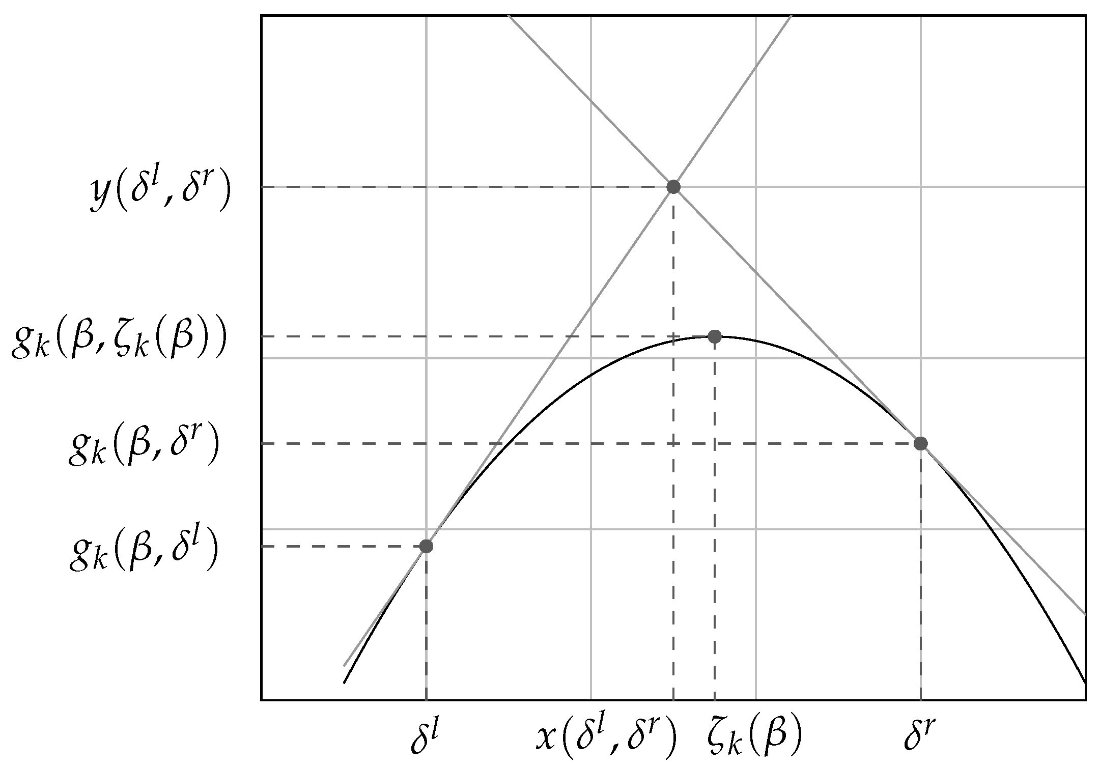
To better follow this proof, the reader may refer to the graphical illustration provided in Figure 2. The lower bound to $G_k\left(\beta \right)$, in Equation (34), trivially follows from the fact that $G_k\left(\beta \right)$ is the maximum value of $g_k(\beta ,\delta )$, for $0\le \delta \le \beta /2$. To establish the upper bound, let $x({\delta }^l,{\delta }^r)$ be the abscissa of the intersection of the tangents (gray lines in Figure 2) considered in the statement (these tangents do intersect, since they have different slopes). Due to the downward convexity (${\displaystyle \frac{{\partial }^2{g}_k}{{\partial }^2\delta }}<0$) of $g_k(\beta ,\delta )$, for any $\delta \in [{\delta }^l,x({\delta }^l,{\delta }^r)]$, the graph of $g_k(\beta ,\delta )$ lies below the tangent at $(\beta ,{\delta }^l)$. Symmetrically, for any $\delta \in [x({\delta }^l,{\delta }^r),{\delta }^r]$, the graph of $g_k(\beta ,\delta )$ lies below the tangent at $(\beta ,{\delta }^r)$. Hence, for any $\delta \in [{\delta }^l,{\delta }^r]$, the graph of $g_k(\beta ,\delta )$ lies below the ordinate $y({\delta }^l,{\delta }^r)$ of the intersection of the two tangents. In particular, $G_k\left(\beta \right)=g_k(\beta ,{\zeta }_k\left(\beta \right))\le y({\delta }^l,{\delta }^r)$, since ${\zeta }_k\left(\beta \right)\in [{\delta }^l,{\delta }^r]$. □

Proposition 10

(Computability of $G_k$, in the infinite precision model). There is a procedure (described in the proof) which, given as inputs an integer $k\ge 2$ and two real values $\beta \in [0,1]$ and $ϵ>0$, outputs an interval $[G^{\prime },G^{″}]$ such that $G_k\left(\beta \right)\in [G^{\prime },G^{″}]$ and $G^{″}-G^{\prime }<ϵ$.

Proof. 

The proposed procedure distinguishes 2 cases.

Case 1: ${\displaystyle \frac{\partial g_k}{\partial \delta }}(\beta ,\beta /4)=0$. Here, $\beta /4={arg\; max}_{\delta }{g}_k(\beta ,\delta )$, whence $G_k\left(\beta \right)=g_k(\beta ,\beta /4)$. The procedure outputs $G^{\prime }=G^{″}=g_k(\beta ,\beta /4)$, clearly satisfying the requirements in the statement.

Case 2: ${\displaystyle \frac{\partial g_k}{\partial \delta }}(\beta ,\beta /4)\ne 0$. Here the procedure includes two phases. In a first phase, a bisection process determines two points, ${\delta }_0^l$ and ${\delta }_0^r$, which satisfy the assumptions of Proposition 9. (For simplicity, the dependence of ${\delta }_0^l$ and ${\delta }_0^r$ upon k and $\beta$ is not made explicit in the notation.) In a second phase, the interval $[{\delta }_0^l,{\delta }_0^r]$ is iteratively bisected, until the interval appearing in Equation (34) has size smaller than $ϵ$. In both phases, the bisection is driven by the sign of ${\displaystyle \frac{\partial g_k}{\partial \delta }}$. The first phase includes two subcases:

Subcase 2a: ${\displaystyle \frac{\partial g_k}{\partial \delta }}(\beta ,\beta /4)>0$. We define the sequence ${\mu }_j=(1-2^{-j})(\beta /2)$, for $j\ge 1$. Letting $h=min\{j\ge 2:{\displaystyle \frac{\partial g_k}{\partial \delta }}(\beta ,{\mu }_j)<0\}$, we set $[{\delta }_0^l,{\delta }_0^r]=[{\mu }_{h-1},{\mu }_h]$.

Subcase 2b: ${\displaystyle \frac{\partial g_k}{\partial \delta }}(\beta ,\beta /4)<0$. We define the sequence ${\nu }_j=2^{-j}(\beta /2)$, for $j\ge 1$. Letting $h=min\{j\ge 2:{\displaystyle \frac{\partial g_k}{\partial \delta }}(\beta ,{\nu }_j)>0\}$, we set $[{\delta }_0^l,{\delta }_0^r]=[{\nu }_h,{\nu }_{h-1}]$.

Since ${lim}_{j\to \infty }{\mu }_j=\beta /2$ and ${lim}_{j\to \infty }{\nu }_j=0$, the interval $[{\delta }_0^l,{\delta }_0^r]$ is well defined, in either subcase. Its endpoints can be computed by iteratively testing the condition on the derivative for $j=1,2,\dots$, till it is satisfied.

In both subcases, ${\zeta }_k\left(\beta \right)\in [{\delta }_0^l,{\delta }_0^r]$. We can then construct a sequence of intervals, each half the size of the preceding one and containing ${\zeta }_k\left(\beta \right)$, as follows.

For $i=1,2,\dots$ do:

• $c_i=({\delta }_{i-1}^l+{\delta }_{i-1}^r)/2$.
• If ${\displaystyle \frac{\partial g_k}{\partial \delta }}(\beta ,c_i)=0$, then set $G^{\prime }=G^{″}=g_k(\beta ,c_i)$ and exit.
• If ${\displaystyle \frac{\partial g_k}{\partial \delta }}(\beta ,c_i)>0$, then let $[{\delta }_i^l,{\delta }_i^r]=[c_i,{\delta }_{i-1}^r]$.
• If ${\displaystyle \frac{\partial g_k}{\partial \delta }}(\beta ,c_i)<0$, then let $[{\delta }_i^l,{\delta }_i^r]=[{\delta }_{i-1}^l,c_i]$.
• Set $G^{\prime }=max(g_k(\beta ,{\delta }_i^l),g_k(\beta ,{\delta }_i^r))$ and $G^{″}=y({\delta }_i^l,{\delta }_i^r)$, as defined in Proposition 9. If $G^{″}-G^{\prime }<ϵ$, then exit.

It is straightforward to show that, for any $\eta >0$, ${log}_2(1/\eta )$ bisection iterations (counting those of both phases) are sufficient to guarantee ${\delta }^r-{\delta }^l\le \eta$, hence to determine ${\zeta }_k\left(\beta \right)$ with accuracy $\eta >0$.

It remains to show that the above for loop is eventually exited. If the loop is exited at step 2, then we are are done. Otherwise, as we will argue, $G^{″}-G^{\prime }$ vanishes with ${\delta }^r-{\delta }^l$ so that, for some i, $G^{″}-G^{\prime }<ϵ$, hence the loop is eventually exited, at step 5. Toward this conclusion, we can observe that

$$\begin{array}{cc}\hfill y({\delta }^l,{\delta }^r)-g_k(\beta ,{\delta }^l)& \le \left|{\displaystyle \frac{\partial g_k}{\partial \delta }}(\beta ,{\delta }^l)\right|(x({\delta }^l,{\delta }^r)-{\delta }^l),\hfill \\ \hfill y({\delta }^l,{\delta }^r)-g_k(\beta ,{\delta }^r)& \le \left|{\displaystyle \frac{\partial g_k}{\partial \delta }}(\beta ,{\delta }^r)\right|({\delta }^r-x({\delta }^l,{\delta }^r)),\hfill \end{array}$$

where $x({\delta }^l,{\delta }^r)$ is the abscissa of the intersection of the tangents. As ${\delta }^r-{\delta }^l$ approaches 0, we have that

$$\begin{array}{cc}\hfill & lim{\delta }^l=lim{\delta }^r=limx({\delta }^l,{\delta }^r)={\zeta }_k\left(\beta \right),\hfill \\ & lim{\displaystyle \frac{\partial g_k}{\partial \delta }}(\beta ,{\delta }^l)=lim{\displaystyle \frac{\partial g_k}{\partial \delta }}(\beta ,{\delta }^r)=0,\hfill \\ & lim{G}^{″}-G^{\prime }=limy({\delta }^l,{\delta }^r)-max(g_k(\beta ,{\delta }^l),g_k(\beta ,{\delta }^r))=0.\hfill \end{array}$$

□

6.4.2. Computing $\mathrm{sign}\left(G_k\left(\beta \right)\right)$

We now consider the more realistic model where only rational numbers are represented, and only arithmetic operations and comparisons with rational inputs can be computed exactly. If $f\left(x\right)$ is a real function of the real variable x, we will restrict our attention to rational inputs and be interested in computing arbitrary approximations of $f\left(x\right)$. More specifically, our target is an approximation algorithm ${\mathcal{A}}_f(x,ϵ)$ of the rational inputs x and $ϵ>0$, whose output $\tilde{f}(x,ϵ)$ satisfies the relationship $|\tilde{f}(x,ϵ)-f\left(x\right)|<ϵ$. Thus, $f\left(x\right)$ is a computable real number, in the sense of Definition 1. These notions naturally extend to functions of several variables.

Approximation algorithms are well known for ${log}_{2}x$, such as the iterative method of [37]. For evaluating a finite arithmetic expression, a tedious but straightforward analysis of error propagation will determine the required accuracy of each intermediate calculation capable of guaranteeing the desired accuracy for the target result. Therefore, approximation algorithms can be derived for $g_k(\beta ,\delta )$ and ${\displaystyle \frac{\partial g_k}{\partial \delta }}(\beta ,\delta )$.

One issue we need to deal with is that an algorithm to compute $f\left(x\right)$ with any desired accuracy does not automatically translate into an algorithm to systematically determine the sign (positive, negative, or zero), of $f\left(x\right)$, denoted $\mathrm{sign}\left(f\right(x\left)\right)$. In fact, while $\tilde{f}(x,ϵ)\ge +ϵ$ implies $f\left(x\right)>0$ and $\tilde{f}(x,ϵ)\le -ϵ$ implies $f\left(x\right)<0$, in the remaining case, $|\tilde{f}(x,ϵ)|<ϵ$, nothing can be inferred about $\mathrm{sign}\left(f\right(x\left)\right)$. On the one hand, when $f\left(x\right)=0$, this “undeterminate” case is bound to occur, for any $ϵ>0$. On the other hand, when $f\left(x\right)\ne 0$, this case will not occur if $ϵ\le \left|f\right(x\left)\right|/2$, since $|\tilde{f}(x,ϵ)-f\left(x\right)|<ϵ\le |f\left(x\right)|/2$ implies $|\tilde{f}(x,ϵ)|\ge |f\left(x\right)|/2\ge ϵ$.

The preceding observations suggest the following procedure $\mathcal{S}({\mathcal{A}}_f,x)$ which, building on an algorithm ${\mathcal{A}}_f$ that computes an approximation $\tilde{f}(x,ϵ)$ to $f\left(x\right)$, will halt and output $\mathrm{sign}\left(f\right(x\left)\right)\in \{-,+\}$, when $f\left(x\right)\ne 0$ and will not halt when $f\left(x\right)=0$. Given a monotonically vanishing, computable sequence ${ϵ}_1,{ϵ}_2,\dots$ (e.g., ${ϵ}_i=2^{-i}$), for $i=1,2,\dots$, the procedure $\mathcal{S}$ computes ${\tilde{f}}_i=\tilde{f}(x,{ϵ}_i)$ by a call to ${\mathcal{A}}_f(x,{ϵ}_i)$; if ${\tilde{f}}_i\ge {ϵ}_i$ or ${\tilde{f}}_i\le -{ϵ}_i$, then it returns $\mathrm{sign}\left({\tilde{f}}_i\right)$ and halts.

The bisection procedure has to be modified so that it will not get stuck in the attempt of evaluating the sign of a zero. Assuming that f has a unique zero in the interval $[a,b]$, say, with $f\left(a\right)<0$ and $f\left(b\right)>0$, a point c where to split the interval can be found as follows. Let $c^{\prime }=(2a+b)/3$ and $c^{″}=(a+2b)/3$ the points that trisect the interval. Interleave the executions of the calls $\mathcal{S}({\mathcal{A}}_f,c^{\prime })$ and $\mathcal{S}({\mathcal{A}}_f,c^{″})$ until the termination of one of them, an event guaranteed to occur since at least one between $f\left(c^{\prime }\right)$ and $f\left(c^{″}\right)$ differs form zero. Let c be the argument for which the execution has terminated, whence $\mathrm{sign}\left(f\right(c\left)\right)$ has been determined. The refined interval is chosen to be $[a,c]$ when $f\left(c\right)>0$ and $[c,b]$ when $f\left(c\right)<0$. In all cases, the interval size shrinks at least by $2/3$.

With the tools we have introduced, we can now tackle the finite-precision computation of $\mathrm{sign}\left(G_k\left(\beta \right)\right)$, a quantity that will play a key role in the computation of ${\beta }_k^{*}$ discussed in the next subsection.

Proposition 11

(Partial computability of $\mathrm{sign}\left(G_k\left(\beta \right)\right)$, in the finite precision model). There is a procedure (described in the proof) which, given as inputs an integer $k\ge 2$ and two rational values $\beta \in [0,1]$ and $ϵ>0$, outputs $\mathrm{sign}\left(G_k\left(\beta \right)\right)$ and halts, if $G_k\left(\beta \right)\ne 0$, and does not halt, if $G_k\left(\beta \right)=0$.

Proof. 

We obtain the procedure for $\mathrm{sign}\left(G_k\left(\beta \right)\right)$ by adapting the procedure to approximate $G_k\left(\beta \right)$ presented in the proof of Proposition 10. To lighten the notation, throughout this proof, we let $g\left(\delta \right)=g_k(\beta ,\delta )$ and $g^{\prime }\left(\delta \right)={\displaystyle \frac{\partial g_k}{\partial \delta }}(\beta ,\delta )$.

Interleave the executions of the calls $\mathcal{S}({\mathcal{A}}_{g^{\prime }},\beta /4)$ and $\mathcal{S}({\mathcal{A}}_{g^{\prime }},\beta /8)$ until termination of one of them, an event guaranteed to occur since at least one between $g^{\prime }(\beta /4)$ and $g^{\prime }(\beta /8)$ differs form zero. Let ${\delta }_0$ be the argument for which the execution has terminated. If $g^{\prime }\left({\delta }_0\right)>0$, then search for a ${\mu }_h$ such that $g^{\prime }\left({\mu }_h\right)<0$ and let $[{\delta }_0^l,{\delta }_0^r]=[{\delta }_0,{\mu }_h]$. Else $g^{\prime }\left({\delta }_0\right)<0$, search for a ${\nu }_h$ such that $g^{\prime }\left({\nu }_h\right)>0$ and let $[{\delta }_0^l,{\delta }_0^r]=[{\nu }_h,{\delta }_0]$. The search has to interleave the evaluation of two consecutive points in the sequence, to avoid the potential non termination of the execution, which can occur at most at one point.

The sequence $[{\delta }_i^l,{\delta }_i^r]$, for $i=1,2,\dots$, of successive refinements of $[{\delta }_0^l,{\delta }_0^r]$ is then constructed, choosing the splitting point $c_i$ by trisection. Let ${ϵ}_i$ be the error bound such that the call to ${\mathcal{A}}_{g^{\prime }}(c_i,{ϵ}_i)$ has enabled the determination of the sign of $g^{\prime }\left(c_i\right)$. Let also ${\eta }_i=min(2^{-i},{ϵ}_i)$ and compute ${\eta }_i$-approximations $\tilde{g}({\delta }_i^l,{\eta }_i)$, $\tilde{g}({\delta }_i^r,{\eta }_i)$, and $\tilde{y}({\delta }_i^l,{\delta }_i^r,{\eta }_i)$. The conditions that enable determining $\mathrm{sign}\left(G_k\left(\beta \right)\right)$ are as follows:

• If $\tilde{g}({\delta }_i^l,{\eta }_i)\ge {\eta }_i$ or $\tilde{g}({\delta }_i^r,{\eta }_i)\ge {\eta }_i$, then return $\mathrm{sign}\left(G_k\left(\beta \right)\right)=+$ and halt.
• If $\tilde{y}({\delta }_i^l,{\delta }_i^r,{\eta }_i)\le -{\eta }_i$, then return $\mathrm{sign}\left(G_k\left(\beta \right)\right)=-$ and halt.

Indeed, in the first case, the condition implies that $g\left({\delta }_i^l\right)=g_k(\beta ,{\delta }_i^l)>0$ or $g\left({\delta }_i^r\right)=g_k(\beta ,{\delta }_i^r)>0$, which in turn implies $G_k\left(\beta \right)>0$. Conversely, if $G_k\left(\beta \right)>0$, for i large enough, both $g\left({\delta }_i^l\right)$ and $g_k\left({\delta }_i^r\right)$, which are monotonically non decreasing with i, become positive. Since ${\eta }_i$ vanishes with i, it will eventually become sufficiently small to satisfy the condition.

Symmetrically, in the second case, the condition implies that $G_k\left(\beta \right)<0$. Conversely, if $G_k\left(\beta \right)<0$, for i large enough, $y({\delta }_i^l,{\delta }_i^r)$, which decreases with i, becomes negative. Again, ${\eta }_i$ will eventually become sufficiently small to satisfy the condition.

Finally, we observe that if $G_k\left(\beta \right)=0$, then neither condition will ever hold and the procedure will not halt. □

6.4.3. Computing ${\beta }_k^{*}=sup{A}_k$

In this subsection, we will see that the set $A_k$ is an interval, closed on the left and open on the right: specifically, $A_k=[0,{\beta }_k^{*})$. On the one hand, this property of $A_k$ is not surprising, since if ${\beta }^{\prime }$ is a lower bound to ${\alpha }_k$ and $\beta <{\beta }^{\prime }$, then $\beta$ is a lower bound too. On the other hand, the property does require a proof, since membership in $A_k$ is a sufficient, but not necessary condition for $\beta$ to be a lower bound, a scenario compatible with $A_k$ having “holes”, that is, with $G_k\left(\beta \right)$ taking both negative and positive values to the left of ${\beta }_k^{*}$. However, we will argue that $A_k$ has no such holes, since $G_k\left(\beta \right)$ has a unique zero in $[0,1]$ which, by Equation (33), is our target, ${\beta }_k^{*}=sup{A}_k$. We will show this zero to be computable.

Proposition 12.

For every $k\ge 2$, in the interval $0\le \beta \le 1$, the function $G_k\left(\beta \right)$ is increasing and has a unique zero, which equals ${\beta }_k^{*}=sup{A}_k$.

Proof. 

From Lemma 4, we have that $G_k\left(\beta \right)=g_k(\beta ,{\zeta }_k\left(\beta \right))$, where ${\zeta }_k\left(\beta \right)$ is the unique solution of the equation (in $\delta$) ${\displaystyle \frac{\partial g_k}{\partial \delta }}(\beta ,\delta )=0$, so that

$$\begin{array}{c}\hfill {\displaystyle \frac{\partial g_k}{\partial \delta }}(\beta ,{\zeta }_k\left(\beta \right))=0.\end{array}$$

(37)

By the chain rule for the total derivative and the above relationship, we get

$$\begin{array}{cc}\hfill {\displaystyle \frac{\partial G_k}{\partial \beta }}& ={\displaystyle \frac{\partial g_k}{\partial \beta }}(\beta ,{\zeta }_k\left(\beta \right)){\displaystyle \frac{\partial \beta }{\partial \beta }}+{\displaystyle \frac{\partial g_k}{\partial \delta }}(\beta ,{\zeta }_k\left(\beta \right)){\displaystyle \frac{\partial {\zeta }_k\left(\beta \right)}{\partial \beta }}={\displaystyle \frac{\partial g_k}{\partial \beta }}(\beta ,{\zeta }_k\left(\beta \right))\hfill \\ \hfill & ={log}_2(k-1)+H^{\prime }\left({\displaystyle \frac{\beta -2{\zeta }_k\left(\beta \right)}{1-{\zeta }_k\left(\beta \right)}}\right),\hfill \end{array}$$

where the last step follows from Equation (30). After several but simple manipulations and letting $\zeta ={\zeta }_k\left(\beta \right)$, the expression just derived together with Equations (37) and (35) yield the relationship

$$\begin{array}{c}\hfill \left({\displaystyle \frac{2-\beta }{1-\zeta }}\right){\displaystyle \frac{\partial G_k}{\partial \beta }}={log}_2{\displaystyle \frac{k}{k-1}}+2H^{\prime }\left(\zeta \right)-H\left({\displaystyle \frac{\beta -2\zeta }{1-\zeta }}\right)+\left(1-{\displaystyle \frac{\beta -2\zeta }{1-\zeta }}\right){log}_2(k-1).\end{array}$$

(38)

We will argue that the right hand side is positive, for any $\beta \in [0,1]$ and any $\zeta \in [0,\beta /2]$. As easily seen, the only negative term in the right hand side of Equation (38) is $-H\left({\displaystyle \frac{\beta -2\zeta }{1-\zeta }}\right)\ge -1$. A case analysis shows that this negative term is offset by one or more of the remaining terms, yielding a positive sum.

Case 1: $\zeta <1/(1+\sqrt{2})$. Considering that $H^{\prime }$ is monotonically decreasing (see Definition 4), we have

$$\begin{array}{c}\hfill 2H^{\prime }\left(\zeta \right)>2H^{\prime }\left({\displaystyle \frac{1}{1+\sqrt{2}}}\right)=2{log}_2{\displaystyle \frac{1-1/(1+\sqrt{2})}{1/(1+\sqrt{2})}}=2{log}_2\sqrt{2}=1.\end{array}$$

Case 2: $\zeta \ge 1/(1+\sqrt{2})$ and $k\ge 4$. We observe that $\left(1-{\displaystyle \frac{\beta -2\zeta }{1-\zeta }}\right)$ is decreasing with $\beta$ and increasing with $\zeta$, whereas ${log}_2(k-1)$ is increasing with k, whence

$$\begin{array}{c}\hfill \left(1-{\displaystyle \frac{\beta -2\zeta }{1-\zeta }}\right){log}_2(k-1)>\left(1-{\displaystyle \frac{1-2/(1+\sqrt{2})}{1-1/(1+\sqrt{2})}}\right){log}_2\left(3\right)>{\displaystyle \frac{1}{\sqrt{2}}}1.58>1.11\end{array}$$

Case 3: $\zeta \ge 1/(1+\sqrt{2})$ and $k=2$. The right hand side of Equation (38) becomes

$$\begin{array}{c}\hfill 1+2H^{\prime }\left(\zeta \right)-H\left({\displaystyle \frac{\beta -2\zeta }{1-\zeta }}\right),\end{array}$$

which is always positive. In fact, if $\zeta <1/2$, then $2H^{\prime }\left(\zeta \right)>0$ and $1-H\left({\displaystyle \frac{\beta -2\zeta }{1-\zeta }}\right)\ge 0$. On the other hand, if $\zeta =1/2$, then $2H^{\prime }\left(\zeta \right)=0$; furthermore, it must be $\beta =1$ so that $H\left({\displaystyle \frac{\beta -2\zeta }{1-\zeta }}\right)=H\left(0\right)=0$.

Case 4: $\zeta \ge 1/(1+\sqrt{2})$ and $k=3$. Considering that (i) $H^{\prime }\left(\zeta \right)\ge 0$ (for $0\le \zeta \le 1/2)$, (ii) $H\left(x\right)\le 1$ (for any $0\le x\le 1$), and (iii) $\left(1-{\displaystyle \frac{\beta -2\zeta }{1-\zeta }}\right)>{\displaystyle \frac{1}{\sqrt{2}}}$ (as seen in Case 2), Equation (38) implies

$$\begin{array}{c}\hfill \left({\displaystyle \frac{2-\beta }{1-\zeta }}\right){\displaystyle \frac{\partial G_k}{\partial \beta }}\ge {log}_2{\displaystyle \frac{3}{2}}-1+{\displaystyle \frac{1}{\sqrt{2}}}>0.58-1+0.70=0.28>0.\end{array}$$

(39)

Having established that $G_k\left(\beta \right)$ has a positive derivative, hence it is increasing, in the interval $[0,1]$, we now argue the existence of a (unique) zero of $G_k\left(\beta \right)$, by showing that $G_k\left(0\right)<0$ and $G_k\left(1\right)>0$, for every $k\ge 2$.

At $\beta =0$, we simply observe that, by definition (i.e., Equation (32)), we have $G_k\left(0\right)={max}_{0\le \delta \le 0}{g}_k(0,\delta )=g_k(0,0)=-{log}_{2}k<0$, for every $k\ge 2$.

At $\beta =1$, we observe that $G_k\left(1\right)={max}_{0\le \delta \le 1/2}{g}_k(1,\delta )\ge g_k(1,1/k)$ and show that $g_k(1,1/k)>0$, for every $k\ge 2$. We consider the following chain of relationships where, starting from Equation (30), (i) we have dropped the contribution $(1-\delta ){log}_2{\displaystyle \frac{1}{1-\delta }}$ to $H\left(\delta \right)$ and the second entropy term, which are both non-negative; (ii) we have plugged $\beta =1$ and $\delta ={\displaystyle \frac{1}{k}}$; and (iii) we have performed simple algebraic manipulations, also making use of the inequality ${log}_2(1+x)\le \left({log}_{2}e\right)x$:

$$\begin{array}{ccc}\hfill g_k(1,1/k)& \ge & \left(1-2{\displaystyle \frac{1}{k}}\right){log}_2(k-1)-\left(1-{\displaystyle \frac{1}{k}}\right){log}_{2}k+2{\displaystyle \frac{1}{k}}{log}_{2}k\hfill \\ & =& {log}_2{\displaystyle \frac{k-1}{k}}+{\displaystyle \frac{2}{k}}{log}_2{\displaystyle \frac{k}{k-1}}+{\displaystyle \frac{1}{k}}{log}_{2}k\hfill \\ & \ge & -\left({log}_{2}e\right)\left(1-{\displaystyle \frac{2}{k}}\right){\displaystyle \frac{1}{k}}+{\displaystyle \frac{1}{k}}{log}_{2}k\hfill \\ & =& {\displaystyle \frac{1}{k}}\left[{log}_{2}k-\left({log}_{2}e\right)\left(1-{\displaystyle \frac{2}{k}}\right)\right].\hfill \end{array}$$

For $k=2$, the expression within the square bracket evaluates to 1. For $k\ge 3$, it is easy to see that the square bracket is positive, as ${log}_{2}k-\left({log}_{2}e\right)\left(1-{\displaystyle \frac{2}{k}}\right)>{log}_{2}3-{log}_{2}e>0$. In conclusion, for every $k\ge 2$, we have $g_k(1,{\displaystyle \frac{1}{k}})>0$, as claimed.

Finally, given that $G_k\left(\beta \right)$ is increasing with $\beta$, its unique zero is the supremum ${\beta }_k^{*}$ of $A_k$ (cf. Equation (33)). □

We can now present a simple numerical algorithm to approximate ${\beta }_k^{*}$, from below, with any desired accuracy.

Proposition 13.

(Computability of ${\beta }_k^{*}$, in the finite precision model). There is a procedure (outlined in the proof) which, on inputs $k\ge 2$ and $ϵ>0$, outputs a number ${\overline{\beta }}_k^{*}\in [{\beta }_k^{*}-ϵ,{\beta }_k^{*}]$. Clearly, ${\overline{\beta }}_k^{*}\le {\alpha }_k$.

Proof. 

In light of Proposition 12, it is straightforward to develop a trisection procedure that starts with the interval $[0,1]$, is driven by the sign of $G_k\left(\beta \right)$ computed according to Proposition 11, stops after $\lceil {log}_{3/2}{\displaystyle \frac{1}{ϵ}}\rceil$ iterations, and outputs the left endpoint of the current interval containing ${\beta }_k^{*}$, which has size smaller than ${(3/2)}^{-\lceil {log}_{3/2}{\displaystyle \frac{1}{ϵ}}\rceil }\le ϵ$. □

Table 8. Lower bound ${\overline{\beta }}_k^{*}$ to ${\alpha }_k$, for various values of k. With reference to Proposition 13, $ϵ={10}^{-8}$, hence the five digits to the right of the decimal point are guaranteed to be the same as those of ${\beta }_k^{*}$. The simple $1-1/k$ upper bound to ${\alpha }_k$ shows how, for large k, ${\beta }_k^{*}$, is quite close to ${\alpha }_k$.

k	${\overline{\mathit{\beta }}}_{\mathit{k}}^{*}$	$1-1/\mathit{k}$
2	$0.17055$	$0.50000$
3	$0.28366$	$0.66667$
4	$0.35978$	$0.75000$
5	$0.41517$	$0.80000$
6	$0.45776$	$0.83333$
7	$0.49183$	$0.85714$
8	$0.51990$	$0.87500$
16	$0.64475$	$0.93750$
32	$0.73867$	$0.96875$
$2^{10}$	$0.94359$	$0.99902$
$2^{20}$	$0.99686$	$0.99999$
$2^{30}$	$0.99978$	$0.99999$
$2^{40}$	$0.99998$	$0.99999$

reports the lower bound ${\overline{\beta }}_k^{*}$ (approximating ${\beta }_k^{*}$ from below), for a set of values of k. The program we have used is based on a direct implementation of the bisection version of the relevant procedures. For the level of accuracy of the reported results, the precision of standard floating point arithmetic turns out to be sufficient. The execution is rather fast: even the result for $k=2^{40}$ took about 15 milliseconds of core-time to compute, even using a non-optimized, straightforward implementation of the bisection algorithm. As a term of comparison, the table also shows the value of the simple upper bound ${\alpha }_k\le 1-{\displaystyle \frac{1}{k}}$ (from Hamming distance). Considering that, from Proposition 8, ${lim}_{k\to \infty }({\alpha }_k-{\beta }_k)=0$, we see how, as k increases, ${\beta }_k^{*}$ provides an increasingly better approximation (from below) to ${\alpha }_k$. To guarantee the same level of approximation via the lower bound ${\alpha }_k\ge {\alpha }_k\left(n\right)-Q\left(n\right)$, increasing values of n are required, as k increases. Eventually, computing ${\beta }_k^{*}$ becomes less expensive than estimating ${\alpha }_k\left(n\right)$.

7. A Conjecture on the Asymptotic Behavior of ${\mathit{\alpha }}_{\mathit{k}}$

Unlike the previous sections of this paper, the present one is rather speculative and is meant to to take some rather preliminary steps toward the understanding of the asymptotic behavior of ${\alpha }_k$ with k. To focus the exploration, we formulate a specific conjecture, namely that ${lim}_{k\to \infty }(1-{\alpha }_k)k=c_{\alpha }$ for some constant $c_{\alpha }\ge 1$. Essentially, we are conjecturing that the limit is finite. The bound $c_{\alpha }\ge 1$ follows from ${\alpha }_k\le 1-{\displaystyle \frac{1}{k}}$ (the expected Hamming distance per symbol). The discussion below provides context and motivation for the conjecture, and contemplates the more specific hypothesis that $3\le c_{\alpha }\le 4$.

In the context of the LCS problem, ref. [38] have proven the conjecture, proposed by [39], that ${lim}_{k\to \infty }{\gamma }_k\sqrt{k}=2$. As a corollary, we have that, for large k, $1-{\alpha }_k\ge {\gamma }_k\approx {\displaystyle \frac{2}{\sqrt{k}}}$. However, our intuition is that, although for large n and k we can expect an LCS of length approximately ${\displaystyle \frac{2n}{\sqrt{k}}}$, it would be too costly, in terms of insertions and deletions, to align more than $\mathcal{O}\left({\displaystyle \frac{n}{k}}\right)$ matches, so that, ultimately, for large k, we expect ${\alpha }_k\approx 1-{\displaystyle \frac{c_{\alpha }}{k}}.$

We tentatively investigate the conjecture numerically, by considering Monte Carlo estimates of the quantity $c_{\alpha ,k}\left(n\right)=(1-{\alpha }_k\left(n\right))k$. Unfortunately, obtaining such estimates with the required precision presents some challenges.

Since we expect values of $c_{\alpha ,k}\left(n\right)$ not much larger than 1, we need the error on $(1-{\alpha }_k\left(n\right))$, hence on ${\alpha }_k\left(n\right)$, to be a fraction of $1/k$, a constraint that becomes increasingly stringent as k increases. In order to guarantee a sufficient upper bound on the error, based on Proposition 3 and its corollary Equation (17), the necessary values of n and N quickly become prohibitive, as k increases. However, we suspect that these errors bounds do become rather loose, for large k. More specifically, we hypothesize that, for $x,y\in {\sum }_k^n$ with large k, the standard deviation of $d_E(x,y)/n$ can be approximated as $\sqrt{{\displaystyle \frac{1}{kn}}}$. This is based on the intuition that, for large k, the edit distance behaves similarly to the Hamming distance $d_H(x,y)$, whose standard deviation can be easily determined to be $\sqrt{n{\displaystyle \frac{1}{k}}\left(1-{\displaystyle \frac{1}{k}}\right)}\approx \sqrt{{\displaystyle \frac{n}{k}}}$. We have tested this hypothesis by experimentally estimating the standard deviation of $d_E(x,y)/n$, for $n=2^{18}$ and $k=2^{14}$, based on $N=80$ independent pairs of random strings. The estimated value turned out to be $0.14\times {10}^{-4}$, well in line with our assumption that the standard deviation is approximately $\sqrt{{\displaystyle \frac{1}{kn}}}=\sqrt{{\displaystyle \frac{1}{2^{14}{2}^{18}}}}=2^{-16}\approx 0.15\times {10}^{-4}$.

Table 9. Estimates of $c_{\alpha ,k}\left(n\right)=(1-{\alpha }_k\left(n\right))k$, each based on a single random pair ($N=1$) generated independently of the other pairs. In bold face are shown the entries of the table where the (hypothesized) standard deviation of the error $\sqrt{k/n}$ lies in the interval $[0.011,0.250]$.

	n
$\mathit{k}$	${\mathbf{2}}^{\mathbf{17}}$	${\mathbf{2}}^{\mathbf{18}}$	${\mathbf{2}}^{\mathbf{19}}$	${\mathbf{2}}^{\mathbf{20}}$
$2^7$	$\mathbf{3.553}$	$\mathbf{3.552}$	$\mathbf{3.566}$	$\mathbf{3.581}$
$2^8$	$\mathbf{3.617}$	$\mathbf{3.608}$	$\mathbf{3.629}$	$\mathbf{3.635}$
$2^9$	$\mathbf{3.531}$	$\mathbf{3.656}$	$\mathbf{3.658}$	$\mathbf{3.678}$
$2^{10}$	$\mathbf{3.570}$	$\mathbf{3.625}$	$\mathbf{3.654}$	$\mathbf{3.669}$
$2^{11}$	$\mathbf{3.406}$	$\mathbf{3.516}$	$\mathbf{3.668}$	$\mathbf{3.652}$
$2^{12}$	$\mathbf{3.250}$	$\mathbf{3.656}$	$\mathbf{3.625}$	$\mathbf{3.672}$
$2^{13}$	$\mathbf{3.000}$	$\mathbf{3.500}$	$\mathbf{3.500}$	$\mathbf{3.703}$
$2^{14}$	$3.125$	$\mathbf{3.250}$	$\mathbf{3.563}$	$\mathbf{3.672}$
$2^{15}$	$3.000$	$3.500$	$\mathbf{3.750}$	$\mathbf{3.313}$
$2^{16}$	$3.500$	$2.750$	$3.250$	$\mathbf{3.125}$
$2^{17}$	$3.000$	$2.000$	$3.000$	$3.000$
$2^{18}$	$4.000$	$4.000$	$2.000$	$2.500$
$2^{19}$	$0.000$	$2.000$	$2.000$	$1.500$
$2^{20}$	$0.000$	$0.000$	$0.000$	$0.000$

shows estimates of $c_{\alpha ,k}\left(n\right)$ for $n=2^{17},2^{18},2^{19},2^{20}$ and $k=2^7,2^8,\dots ,2^{20}$. Highlighted in bold face are the entries (33 in number) for which the hypothesized statistical error $k\sqrt{{\displaystyle \frac{1}{kn}}}=\sqrt{{\displaystyle \frac{k}{n}}}$ on $c_{\alpha ,k}\left(n\right)$ is at most ${\displaystyle \frac{1}{4}}$, that is, $k\le {\displaystyle \frac{n}{16}}$. We can observe that, where the hypothesized error is small enough, $3\le c_{\alpha ,k}\left(n\right)\le 4$. We remark that, although to cope with the quadratic complexity of the edit distance computation we have considered only one pair of random strings for each $(k,n)$ entry in Table 9, the consistency of the numerical value of $c_{\alpha ,k}\left(n\right)$ across the 33 bold entries, obtained from statistically independently samples, does lend some support to the sub-conjecture $3\le c_{\alpha }\le 4$.

Of course, how well $c_{\alpha ,k}\left(n\right)$ approximates $c_{\alpha ,k}$ depends on how well ${\alpha }_k\left(n\right)$ approximates ${\alpha }_k$. The quality of the latter approximation increases for large k, where the the bound provided by Theorem 2 becomes loose. In fact, putting together various results, we have that

$$1-{\displaystyle \frac{M}{{log}_2(k-1)}}\le {\alpha }_k\le {\alpha }_k\left(n\right)\le 1-{\displaystyle \frac{1}{k}}.$$

(40)

We can see that the difference between the last and the first term, hence the difference ${\alpha }_k\left(n\right)-{\alpha }_k$ between the intermediate terms, vanishes when k diverges. The quantitative impact on the difference $c_{\alpha ,k}-c_{\alpha ,k}\left(n\right)$ remains to be seen, but the relative stability of the bold entries in each column of Table 9 seems compatible with assuming a small impact. Of course, this section remains in the realm of conjectures, which will hopefully provide some motivation for rigorous analysis that may confirm as well as refute them.

8. Conclusions and Further Questions

In this paper, we have explored ways to compute Monte Carlo estimates, upper bounds, and lower bounds to the asymptotic constant characterizing the expected edit distance between random, independent strings. We have presented the theoretical basis for various approaches and used them to obtain numerical results for some alphabet sizes k, which improve over previously known values [1]. However, there is still a significant gap between upper and lower bounds that can be actually computed in a reasonable time. Below, we outline a number of open questions worthy of further investigation.

The approaches proposed here can be extended to the study of other statistical properties of the edit distance for a given length n, e.g., the standard deviation, which has been widely studied in the context of the longest common subsequence. Ultimately, a characterization of the full distribution would be desirable.

The exact rate of convergence $q_k\left(n\right)={\alpha }_k\left(n\right)-{\alpha }_k$, or even just its asymptotic behavior, remains to be determined. In particular, we are not aware of any significant lower bound to $q_k\left(n\right)$ to be compared with the upper bound $Q\left(n\right)$. Moreover, this upper bound is oblivious to k, whereas the rate of convergence is affected by k, as indicated by Equation (40).

From Proposition 8 and a straightforward analysis of “Hamming scripts”, which use only matches and substitutions, we know that ${\displaystyle \frac{M}{{log}_{2}k}}\le 1-{\alpha }_k\le {\displaystyle \frac{1}{k}}$, (where $M\approx 2.52$); what is the exact asymptotic behavior of $1-{\alpha }_k$? We have conjectured that, asymptotically, $1-{\alpha }_k$ approaches $c_{\alpha }/k$, for some constant $c_{\alpha }\ge 1$; but whether the conjecture holds, and if so for which value of $c_{\alpha }$, remains to be seen.

Of mathematical interest, is the question whether ${\alpha }_k$ is a rational or an algebraic number. The answer could depend upon k. The recent work of [19] on the algebraic nature of ${\gamma }_2$ indicates that this line of investigation may lead to uncovering deep combinatorial properties that can shed light on various aspects of the subject, well beyond mere mathematical curiosity.

The analysis of the statistical error could be somewhat improved, if the experimental evidence that the standard deviation of $d_E(x,y)$ is $o\left(\sqrt{n}\right)$ were corroborated analytically. The dependence upon k could also play a role here.

The complexity of computing, say, the most significant h bits of ${\alpha }_k\left(n\right)$ remains a wide open question. The only known lower bound is $\Omega (logk+logn+h)$, based on the input and output size. It is a far cry from the current upper bound, which is doubly exponential in $logn$. However, a deeper understanding of the distribution and symmetries of the edit distance is likely to be required before the computation time of ${\alpha }_k\left(n\right)$ can be significantly improved.

The lower bounds presented in Section 6 are based on upper bounds to the number of optimal scripts of a given cost r. Our counting argument could be refined to take into account some properties of optimal edit scripts. For example, in an optimal script, an insertion cannot immediately precede or follow a deletion (since the same result could be achieved by just one substitution). Furthermore, it would be easy to show that, for many pairs of strings, multiple scripts are counted by our argument. Part of the difficulty with improving script counting comes from the analytical tractability of the resulting combinatorial expressions, which would be far more complicated than Equation (28).

Another potential weakness of our lower bound is that it is derived from a lower bound to $ecc\left(x\right)$ that must hold for every $x\in {\sum }_k^n$. If, as n goes to infinity, the fraction of strings with eccentricity significantly smaller than the average were to remain sufficiently high, then the approach would be inherently incapable of yielding tight bounds. On the other hand, preliminary efforts seem to indicate that characterizing the strings with minimum eccentricity is not straightforward. In contrast, it is a relatively simple exercise to prove that the strings of maximum eccentricity are those where all positions contain the same symbol and that their eccentricity equals $(1-{\displaystyle \frac{1}{k}})n$.

In terms of applications, it would be interesting to explore the role of statistical properties of the edit distance in string alignment and other key problems in DNA processing and molecular biology. One motivation is provided by the error profile of reads coming from third generation sequencers (e.g., PacBio), where sequencing errors can be modeled as edit operations. In this context, it would be important to generalize the analysis to non-uniform string distributions, whether defined analytically or from empirical data, such as the distribution of substrings from the human DNA. As briefly discussed in Section 4 and Section 5, the approach we have presented for Monte Carlo estimates and for exact estimates via the Coalesced Dynamic Programming algorithm can easily handle arbitrary symbol distributions, as long as the symbols are statistically independent. The extension of the lower bounds of Section 6 appears less straightforward.

Also of great interest would be to analyze the expected distance between noisy copies of two independent strings, as well as between a string and a noisy copy of itself, when the noise can be modeled in terms of edit operations.

While it is natural to begin investigating questions in the simplest scenarios, which for the present investigation is represented by strings with independent symbols, in several application contexts, the assumption of independence is not satisfied. Hence, future work should go in the direction of removing this assumption. However, while the experimental evidence may clearly indicate that some sequences exhibit a non trivial degree of intersymbol dependence, for example because they are compressible, such dependence has not been satisfactorily captured by well defined stochastic models. Therefore, it is likely that, in the near future, dependent models will be studied more because they have a well understood structure (say, Markov models) than because the are known to capture natural phenomena. Finding the right models, perhaps based on variants of transformers, is probably the main key step, to enable a better connection between theory and applications.

References

1. Ganguly, S.; Mossel, E.; Racz, M.Z. Sequence assembly from corrupted shotgun reads. arXiv 2016, arXiv:1601.07086. [Google Scholar]
2. Rubinstein, A. Hardness of Approximate Nearest Neighbor Search. In STOC 2018: Proceedings of the 50th Annual ACM SIGACT Symposium on Theory of Computing; Association for Computing Machinery: New York, NY, USA, 2018; pp. 1260–1268. [Google Scholar] [CrossRef]
3. Comin, M.; Schimd, M. Assembly-free genome comparison based on next-generation sequencing reads and variable length patterns. BMC Bioinform. 2014, 15, S1. [Google Scholar] [CrossRef] [PubMed]
4. Weirather, J.L.; de Cesare, M.; Wang, Y.; Piazza, P.; Sebastiano, V.; Wang, X.J.; Buck, D.; Au, K.F. Comprehensive comparison of Pacific Biosciences and Oxford Nanopore Technologies and their applications to transcriptome analysis. F1000Research 2017, 6, 100. [Google Scholar] [CrossRef] [PubMed]
5. Chvátal, V.; Sankoff, D. Longest common subsequences of two random sequences. J. Appl. Probab. 1975, 12, 306–315. [Google Scholar] [CrossRef]
6. Steele, J.M. Probability Theory and Combinatorial Optimization; SIAM: Philadelphia, PA, USA, 1997. [Google Scholar] [CrossRef]
7. Schimd, M.; Bilardi, G. Bounds and estimates on the average edit distance. In Proceedings of the String Processing and Information Retrieval; Brisaboa, N.R., Puglisi, S.J., Eds.; Springer: Cham, Switzerland, 2019; pp. 91–106. [Google Scholar] [CrossRef]
8. Bilardi, G.; Schimd, M. Computable Bounds and Monte Carlo Estimates of the Expected Edit Distance. arXiv 2022, arXiv:2211.07644. [Google Scholar]
9. Rosenfeld, M. Upper bounds on the average edit distance between two random strings. arXiv 2024, arXiv:2407.18113. [Google Scholar] [CrossRef]
10. Bundschuh, R. High precision simulations of the longest common subsequence problem. Eur. Phys. J. B-Condens. Matter Complex Syst. 2001, 22, 533–541. [Google Scholar] [CrossRef]
11. Dancík, V. Expected Length of Longest Common Subsequences. Ph.D. Thesis, University of Warwick, Coventry, UK, 1994. [Google Scholar]
12. Ning, K.; Choi, K.P. Systematic assessment of the expected length, variance and distribution of Longest Common Subsequences. arXiv 2013, arXiv:1306.4253. [Google Scholar]
13. Bukh, B.; Cox, C. Periodic words, common subsequences and frogs. Ann. Appl. Probab. 2022, 32, 1295–1332. [Google Scholar] [CrossRef]
14. Lueker, G.S. Improved Bounds on the Average Length of Longest Common Subsequences. J. ACM 2009, 56, 17. [Google Scholar] [CrossRef]
15. Heineman, G.T.; Miller, C.; Reichman, D.; Salls, A.; Sárközy, G.; Soiffer, D. Improved Lower Bounds on the Expected Length of Longest Common Subsequences. arXiv 2024, arXiv:2407.10925. [Google Scholar]
16. Baeza-Yates, R.A.; Gavaldá, R.; Navarro, G.; Scheihing, R. Bounding the Expected Length of Longest Common Subsequences and Forests. Theory Comput. Syst. 1999, 32, 435–452. [Google Scholar] [CrossRef]
17. Alexander, K.S. The Rate of Convergence of the Mean Length of the Longest Common Subsequence. Ann. Appl. Probab. 1994, 4, 1074–1082. [Google Scholar] [CrossRef]
18. Lember, J.; Matzinger, H.; Torres, F. The rate of the convergence of the mean score in random sequence comparison. Ann. Appl. Probab. 2012, 22, 1046–1058. [Google Scholar] [CrossRef]
19. Tiskin, A. The Chvátal–Sankoff problem: Understanding random string comparison through stochastic processes. In Proceedings of the Representation Theory, Dynamical Systems, Combinatorial Methods, Part XXXIV. Zapiski Nauchnykh Seminarov POMI; Vershik, A.M., Vassiliev, N.N., Eds.; Springer: Berlin/Heidelberg, Germany, 2022; pp. 191–224. [Google Scholar]
20. Masek, W.J.; Paterson, M.S. A faster algorithm computing string edit distances. J. Comput. Syst. Sci. 1980, 20, 18–31. [Google Scholar] [CrossRef]
21. Myers, G. A Fast Bit-Vector Algorithm for Approximate String Matching Based on Dynamic Programming. J. ACM 1999, 46, 395–415. [Google Scholar] [CrossRef]
22. Hirschberg, D.S. A Linear Space Algorithm for Computing Maximal Common Subsequences. Commun. ACM 1975, 18, 341–343. [Google Scholar] [CrossRef]
23. Kundeti, V.; Rajasekaran, S. Extending the four Russian algorithm to compute the edit script in linear space. In Proceedings of the International Conference on Computational Science; Bubak, M., van Albada, G.D., Dongarra, J., Sloot, P.M.A., Eds.; Springer: Berlin/Heidelberg, Germany, 2008; pp. 893–902. [Google Scholar] [CrossRef]
24. Abboud, A.; Backurs, A.; Williams, V.V. Tight Hardness Results for LCS and Other Sequence Similarity Measures. In Proceedings of the 2015 IEEE 56th Annual Symposium on Foundations of Computer Science; IEEE: Piscataway, NJ, USA, 2015; pp. 59–78. [Google Scholar] [CrossRef]
25. Backurs, A.; Indyk, P. Edit Distance Cannot Be Computed in Strongly Subquadratic Time (Unless SETH is False). In STOC ’15: Proceedings of the Forty-Seventh Annual ACM Symposium on Theory of Computing. Association for Computing Machinery; Association for Computing Machinery: New York, NY, USA, 2015; pp. 51–58. [Google Scholar] [CrossRef]
26. Ukkonen, E. Algorithms for approximate string matching. Inf. Control 1985, 64, 100–118. [Google Scholar] [CrossRef]
27. Landau, G.M.; Myers, E.W.; Schmidt, J.P. Incremental String Comparison. SIAM J. Comput. 1998, 27, 557–582. [Google Scholar] [CrossRef]
28. Andoni, A.; Krauthgamer, R.; Onak, K. Polylogarithmic Approximation for Edit Distance and the Asymmetric Query Complexity. In Proceedings of the 2010 IEEE 51st Annual Symposium on Foundations of Computer Science; IEEE: Piscataway, NJ, USA, 2010; pp. 377–386. [Google Scholar] [CrossRef]
29. Chakraborty, D.; Das, D.; Goldenberg, E.; Koucky, M.; Saks, M. Approximating Edit Distance within Constant Factor in Truly Sub-Quadratic Time. In Proceedings of the 2018 IEEE 59th Annual Symposium on Foundations of Computer Science; IEEE: Piscataway, NJ, USA, 2018; pp. 979–990. [Google Scholar] [CrossRef]
30. Chakraborty, D.; Das, D.; Goldenberg, E.; Kouckỳ, M.; Saks, M. Approximating edit distance within constant factor in truly sub-quadratic time. J. ACM 2020, 67, 36. [Google Scholar] [CrossRef]
31. Rubinstein, A.; Song, Z. Reducing approximate Longest Common Subsequence to approximate Edit Distance. In Proceedings of the 2020 ACM-SIAM Symposium on Discrete Algorithms (SODA); SIAM: Philadelphia, PA, USA, 2020; pp. 1591–1600. [Google Scholar] [CrossRef]
32. Calvo-Zaragoza, J.; Oncina, J.; de la Higuera, C. Computing the Expected Edit Distance from a String to a Probabilistic Finite-State Automaton. Int. J. Found. Comput. Sci. 2017, 28, 603–621. [Google Scholar] [CrossRef]
33. Boche, H.; Böck, Y.; Deppe, C. On the Effectiveness of Fekete’s Lemma in Information Theory. In Proceedings of the 2020 IEEE Information Theory Workshop (ITW); IEEE: Piscataway, NJ, USA, 2021; pp. 1–5. [Google Scholar] [CrossRef]
34. Spencer, J. Asymptopia; American Mathematical Society: Providence, RI, USA, 2014. [Google Scholar] [CrossRef]
35. McDiarmid, C. On the method of bounded differences. Surv. Comb. 1989, 141, 148–188. [Google Scholar] [CrossRef]
36. Bhardwaj, V.; Pevzner, P.A.; Rashtchian, C.; Safonova, Y. Trace Reconstruction Problems in Computational Biology. IEEE Trans. Inf. Theory 2021, 67, 3295–3314. [Google Scholar] [CrossRef] [PubMed]
37. Majithia, J.C.; Levan, D. A note on base-2 logarithm computations. Proc. IEEE 1973, 61, 1519–1520. [Google Scholar] [CrossRef]
38. Kiwi, M.; Loebl, M.; Jiří, M. Expected length of the longest common subsequence for large alphabets. Adv. Math. 2005, 18, 480–498. [Google Scholar] [CrossRef]
39. Sankoff, D.; Kruskal, J. Common Subsequences and Monotone Subsequences. In Time Warps, String Edits, and Macromolecules: The Theory and Practice of Sequence Comparison; Addison-Wesley Publishing Company: Reading, MA, USA, 1983; pp. 363–365. [Google Scholar]
Figure 1. Comparison between estimates α ˜ 4 ( n , N ) of α k ( n ) (blue dots) and estimates α ^ 4 ( n , N ) of α 4 (orange crosses). For each value, the confidence interval is shown.
Information 17 00685 g001
Figure 2. Illustration of the proof of Proposition 9.
Information 17 00685 g002