Article

Non-Gaussian Quadrature Integral Transform Solution of Parabolic Models with a Finite Degree of Randomness

by
María-Consuelo Casabán
1,2,†,
Rafael Company
1,2,† and
Lucas Jódar
1,2,*,†
1
Instituto Universitario de Matemática Multidisciplinar, Building 8G, access C, 2nd floor, 46022 Valencia, Spain
2
Universitat Politècnica de València, Camino de Vera s/n, 46022 Valencia, Spain
*
Author to whom correspondence should be addressed.
These authors contributed equally to this work.
Mathematics 2020, 8(7), 1112; https://doi.org/10.3390/math8071112
Submission received: 13 June 2020 / Revised: 1 July 2020 / Accepted: 3 July 2020 / Published: 6 July 2020
(This article belongs to the Special Issue Stochastic Differential Equations and Their Applications 2020)

Abstract

:
In this paper, we propose an integral transform method for the numerical solution of random mean square parabolic models, that makes manageable the computational complexity due to the storage of intermediate information when one applies iterative methods. By applying the random Laplace transform method combined with the use of Monte Carlo and numerical integration of the Laplace transform inversion, an easy expression of the approximating stochastic process allows the manageable computation of the statistical moments of the approximation.

1. Introduction

Since the seminal works [1,2], random uncertainty has gained presence in the mathematical models as a way to fit better the real world. The  parameters, coefficients and initial/boundary conditions in real problems are subject to uncertainties, not only by error measurement but also due to the lack of access to the measurement or the heterogeneity of the media; see [3,4] for applications. However, successful approaches used to deal with deterministic problems are not appropriated to manage random models. In particular, this occurs with iterative methods. The reason is that in the solution of random models, it is not enough to provide the solution stochastic process (s.p.), but also the computation of its statistical moments such as the expectation and the variance. Iterative processes involve the storage of intermediate operational random calculus becoming unmanageable. This motivates the search of alternative approaches allowing an easy formal expression of the approximating s.p. solution making possible the computation of its statistical moments. Integral transform method is an efficient approach dealing with both deterministic and random partial differential models when they are combined with quadrature rules to approximate the final infinite integral linked to the inverse integral transform solution [5,6]. Random uncertainty can be modelled in several ways depending of the use of Brownian motion stochastic processes (s.p.’s) and Itô calculus, or other s.p.’s and the mean square (m.s.) calculus [7]. We follow the m.s. approach because of two main advantages, the first is that the m.s. approach coincides with the deterministic, when the random model is supposed to be deterministic [8]. The second is that when an s.p. is m.s. close to another one, then its expectation and its variance are also close [6].
The use of an integral transform needs to be combined with certain appropriate numerical integration technique for the numerical inversion. The quadrature integration method should take care of the oscillatory behaviour of the integrand, and it suggests avoiding Gaussian-quadrature rules used in [6]; see also [9,10,11]. Although the integral transform method has been mainly used for constant coefficient partial differential models [12] in the deterministic framework, because it underlies the assumption that the transformed ordinary differential problem needs to be solved explicitly, and this is not the case; see [13]. This approach has been used for the random case in [5,6,8] for both the constant coefficient and variable coefficient random m.s. case. Apart from the coefficients, the randomness may appear into the initial/boundary conditions. The uncertainty into the model is based on impurities of materials, heterogeneities in the media, error measurements or the lack/difficulty of access to measurements; see [6] and references therein.
This paper deals with random parabolic partial differential models of the form
u ( x , t ) t = x p ( x ) u ( x , t ) x q ( x ) u ( x , t ) + Φ ( x , t ) , x > 0 , t > 0 ,
u ( 0 , t ) = f 1 ( t ) , t > 0 ,
u ( 0 , t ) x = f 2 ( t ) , t > 0 ,
u ( x , 0 ) = g ( x ) , x > 0 ,
u ( x , t ) remains bounded as x , t > 0 ,
with appropriate additional conditions on the random coefficients p ( x ) and q ( x ) , the random source term Φ ( x , t ) , and the random initial/boundary conditions s.p.’s, g ( x ) , f 1 ( t ) and f 2 ( t ) to be specified later, in the framework of uncertainty models with a finite degree of randomness [8,14], that is, the s.p.’s are functions depending on a finite number of random variables (r.v.’s). The model (1)–(5) is frequent in heat and mass transfer theory and chemical engineering sciences, [15], ([16] p. 388).
This paper is organized as follows. Section 2 includes some notations, definitions and preliminary results, about the mean square calculus of random differential equations and random Laplace transform, as well as the construction of the formal s.p. solution of problem (1)–(5). In Section 3, we construct firstly an approximation s.p. solution by truncating the infinite integral Laplace inversion. Then, non-Gaussian random quadrature formulae allow the approximating s.p. as a sum whose expectation and variance are easily computable. Numerical procedure algorithms to construct the numerical approximation are also included. In Section 4, numerical simulations which combine the use of Monte Carlo method and the numerical integration of the Laplace transform inversion are made to check the efficiency of the proposed numerical methods.

2. Preliminaries and Formal Solution

In order to be comprehensive but not exhaustive we recall some notation, definitions and results about m.s. calculus and random Laplace transform; see [8]. Let ( Ω , F , R ) be a complete probability space, and let L p m × n ( Ω ) be the set of all random matrices Y = ( y i j ) m × n whose entries y i j are random variables (r.v.’s) satisfying
y i j p = E [ | y i j | p ] 1 / p < + , p 1 ,
what this means is that y i j L p ( Ω ) , where E [ · ] denotes the expectation operator. The space of all random matrices of size m × n , endowed with the matrix p-norm, L p m × n ( Ω ) , defined by
Y p = i = 1 m j = 1 n y i j p , E [ | y i j | p ] < + ,
is a Banach space. This definition of the matrix p norm can be extended to matrix s.p.’s Y ( t ) = y i j ( t ) m × n of L p m × n ( Ω ) , where now each entry y i j ( t ) L p ( Ω ) for every 1 i m , 1 j n . The definitions of integrability, continuity, differentiability of a matrix function lying in L p m × n ( Ω ) follows in a natural manner using matrix p norm introduced above. The case mean square corresponds to p = 2 , and mean four p = 4 . One has L 4 m × n ( Ω ) L 2 m × n ( Ω ) ; see [6].
Definition 1.
C is the class of all the 2-s.p.’s h ( t ) defined in the real line such that:
(i) 
h ( t ) is m.s. locally integrable,
(ii) 
h ( t ) = 0 , if t < 0 ,
(iii) 
The 2-norm of h ( t ) is of exponential order, i.e., there exist real constants c 0 , called the abscissa of convergence, and  M > 0 such that
h ( t ) 2 M e c t , t 0 .
Taking into account Definition 1, the random Laplace transform of a 2-s.p. h ( t ) C is defined by the m.s. integral
H ( s ) = L [ h ( t ) ] ( s ) = 0 h ( t ) e s t d t , s C , Re ( s ) > c 0 ,
see [8]. Furthermore, if  h ( t ) is a s.p., that is, h ( t ) is m.s. differentiable, and  h ( t ) belongs to class C , then
L [ h ( t ) ] ( s ) = s L [ h ( t ) ] ( s ) h ( 0 + ) ,
see [8]. If we know H ( s ) = L [ h ( t ) ] ( s ) , then the random inverse transform allows to recover h ( t ) in terms of H ( s ) :
h ( t ) = 1 2 π i α i α + i H ( s ) e s t d s , t > 0 , α > c ,
where i denotes the imaginary unit. Now assume that the coefficient p ( x ) in (1) is a 2-s.p. m.s differentiable so that the m.s. derivative
x p ( x ) u ( x , t ) x = p ( x ) 2 u ( x , t ) x 2 + p ( x ) u ( x , t ) x ,
and (1) can be written for x > 0 , t > 0 ,
u ( x , t ) t = p ( x ) 2 u ( x , t ) x 2 + p ( x ) u ( x , t ) x q ( x ) u ( x , t ) + Φ ( x , t ) .
Let us assume that Equation (10) has a solution 2-s.p. u ( x , t ) regarded as a function of active variable t, lies in the class C , u ( x , · ) and let
U ( x ) ( s ) = L u ( x , · ) ( s ) .
Assume that the source term Φ ( x , t ) is also a 2-s.p. in class C for each fixed x > 0 , so that it is well defined
Ψ ( x ) ( s ) = L Φ ( x , · ) ( s ) .
Formal application of random Laplace transform to both sides of Equation (10), using property (8), (11), (12) and assuming that Leibniz rule for the derivative of an integral (see [17]), holds true, one has
s U ( x ) ( s ) u ( x , 0 ) = p ( x ) 2 U ( x ) x 2 ( s ) + p ( x ) U ( x ) x ( s ) q ( x ) U ( x ) ( s ) + Ψ ( x ) ( s ) .
Let us assume that the 2-s.p. p ( x ) has positive realizations for almost every (a.e.) event ξ Ω , i.e.,
p ( x , ξ ) = f ( x ) δ ( ξ ) > 0 , ( a . e . ) ξ Ω , x > 0 .
Under hypothesis (14), using (4) and (13), we can write (13) in the more compact form, random ordinary differential equation in the variable x:
2 U ( x ) x 2 ( s ) + p ( x ) p ( x ) U ( x ) x ( s ) q ( x ) + s p ( x ) U ( x ) ( s ) = Ψ ( x ) ( s ) + g ( x ) p ( x ) , x > 0 .
Assume that the random boundary conditions f 1 ( t ) and f 2 ( t ) are also 2-s.p.’s in class C , so by applying random Laplace transform to both sides of (2) and (3), admitting Leibniz rule for the derivative of an integral, one has
U ( 0 ) ( s ) = F 1 ( s ) , U ( 0 ) x ( s ) = F 2 ( s ) ,
where we have denoted F 1 ( s ) = L f 1 ( t ) ( s ) and F 2 ( s ) = L f 2 ( t ) ( s ) .
The m.s. random differential problem (15) and (16) is transformable into extended first order random initial value problem in the unknown Y ( x ) ( s ) = [ U ( x ) ( s ) , U ( x ) ( s ) ] T in the variable x:
Y ( x ) ( s ) = A ( x ) ( s ) Y ( x ) ( s ) + B ( x ) ( s ) , x > 0 Y ( 0 ) ( s ) = F 1 ( s ) F 2 ( s ) = F ( s ) ,
where
A ( x ) ( s ) = 0 1 q ( x ) + s p ( x ) p ( x ) p ( x ) ; B ( x ) ( s ) = 0 Ψ ( x ) ( s ) + g ( x ) p ( x ) .
In order to guarantee the existence of a m.s. solution s.p., one needs that entries of the random matrix A ( x ) ( s ) satisfies the moment condition of [18] for every x > 0 , that is
E a i , j ( x ) r m i , j ( h i , j ) r < + , r 0 , 1 i , j 2 ,
and the entries of B ( x ) ( s ) are 4-integrable and lie in L 4 ( Ω ) see [18]. In our case, this means that each s.p.
q ( x ) p ( x ) , 1 p ( x ) , p ( x ) p ( x ) satisfy the moment condition ( 19 )
and
Ψ ( x ) ( s ) + g ( x ) p ( x ) lies in L 4 ( Ω ) and is 4 integrable .
Under conditions (19)–(21), assuming that the random vector initial condition verifies
F ( s ) L 4 ( Ω ) ,
there is a m.s. solution s.p. of (17) given by
Y ( x ) ( s ) = Φ A ( x ; 0 ) F ( s ) + 0 x Φ A 1 ( v ; 0 ) B ( v ) d v ,
where Φ A ( x ; 0 ) is the random fundamental matrix solution of the random homogeneous matrix differential problem:
W ( x ) ( s ) = A ( x ) ( s ) W ( x ) ( s ) , W ( 0 ) = I ,
with A ( x ) ( s ) the random matrix defined in (18); see [18]. Following with the construcction of the formal m.s. solution of the problem (10), (2)–(5), using the random Laplace inverse Formula (9) and denoting
U ( x ) ( s ) = [ 1 , 0 ] Y ( x ) ( s ) ,
it follows that
u ( x , t ) = 1 2 π i α i α + i U ( x ) ( s ) e s t d s = 1 2 π i α i α + i [ 1 , 0 ] Y ( x ) ( s ) e s t d s ,
where Y ( x ) ( s ) is given by (23). Note that the convergence of the integral (26) holds true if
+ Y ( x ) ( α + i v ) d v < + , α > c 0 .
The next step is the approximation of the s.p. u ( x , t ) given by the numerical treatment of (26), so that its expression makes manageable the computation of its statistical moments. For the sake of accuracy for long time domain and the oscillatory character of the integrand, Gaussian quadrature is not advisable. As  u ( x , t ) is a real s.p., taking advantage of the relationship between the inverse Laplace transform and Fourier cosine integrals (see [19] and ([20] p. 28)) we can write
u ( x , t ) = 2 e α t π 0 Re [ U ( x ) ( α + i w ) ] cos ( w t ) d w ,
and using (25)
u ( x , t ) = 2 e α t π 0 Re Y ( x ) ( α + i w ) cos ( w t ) d w .

3. Random Numerical Solutions

Under hypothesis (27) the random integral (26) is m.s. convergent and the truncated s.p. approximate solution takes the form
u ˜ R ( x , t ) = 2 e α t π [ 1 , 0 ] 0 R Re Y ( x ) ( α + i w ) cos ( w t ) d w ,
where R approaches infinity and Y ( x ) is the solution s.p. of the random initial value problem (17). Let us write (29) in the following form for each realization ξ Ω
u ˜ R ( x , t ) ( ξ ) = 2 e α t π [ 1 , 0 ] I R [ Y ( x , ξ ) , t , α ] .
Let us consider the partition of the interval [ 0 , R ] given by M + 1 points w j = k j , so that k = Δ w = R M , 0 j M . Using the random trapezoidal quadrature inspired in ([10] Section 3.5) one approximates I R [ Y ( x , ξ ) , t , α ] by
I R [ Y ( x , ξ ) , t , α ] 1 2 Re [ Y ( x , ξ ) ( α ) ] + k j = 1 M Re Y ( x , ξ ) ( α + i w j ) cos ( w j t ) ,
where the half weight is omitted at the right end due to the infinite nature of the original domain [ 0 , + ) ; see [19].
From (30) and (31) and taking into account all the realizations ξ Ω , one gets the approximate s.p. solution of the problem (1)–(5) given by
u R , k ( x , t ) = 2 e α t k π [ 1 , 0 ] 1 2 Re Y ( x ) ( α ) + j = 1 M Re Y ( x ) ( α + i w j ) cos ( w j t ) , w j = k j , 0 j M .
Taking expectations in (32) one has
E u R , k ( x , t ) = 2 e α t k π [ 1 , 0 ] 1 2 E Re [ Y ( x ) ( α ) ] + j = 1 M E Re Y ( x ) ( α + i w j ) cos ( w j t ) ,
and the corresponding variance
Var u R , k ( x , t ) = E u R , k ( x , t ) 2 E u R , k ( x , t ) 2 = 4 e 2 a t k 2 π 2 [ 1 , 0 ] j = 0 M = 0 M γ j γ cos ( w j t ) cos ( w t ) Cov Re Y ( x ) ( α + i w j ) , Re Y ( x ) ( α + i w ) ,
where
γ 0 = 1 2 , γ j = 1 , 1 j M ,
and Cov [ P , Q ] = E [ P Q ] E [ P ] E [ Q ] .
Note that the m.s. solution Y ( x ) ( · ) involved in (32), given by (23), is not available except in a limited number of cases, see Example 5 of [18], because the random fundamental matrix Φ A ( x ; 0 ) is not known. This motivates, from a practical point of view, the search of alternative approximations via simulations, the so called Monte Carlo approach [21]. Although it is well-known that the speed of convergence of Monte Carlo method is rather slow [22], it is a useful tool for our random problem in combination with random integral transform methods and numerical integration techniques. Monte Carlo method provides the E R e [ Y ( x ) ( · ) ] throughout the average of an appropriate number of realizations ξ Ω of the deterministic problem
Y ( x , ξ ) ( s ) = A ( x , ξ ) ( s ) Y ( x , ξ ) ( s ) + B ( x , ξ ) ( s ) , x > 0 Y ( 0 , ξ ) ( s ) = F ( ξ ) ( s ) ,
Then the expectation and its corresponding variance by K-Monte Carlo (MC) simulations are computed by the following expressions
E MC K u R , k ( x , t ) = 2 e α t k π [ 1 , 0 ] 1 2 E MC K Re [ Y ( x ) ( α ) ] + j = 1 M E MC K Re Y ( x ) ( α + i w j ) cos ( w j t ) ,
and
Var MC K u R , k ( x , t ) = E MC K u R , k ( x , t ) 2 E MC K u R , k ( x , t ) 2 = 4 e 2 a t k 2 π 2 [ 1 , 0 ] j = 0 M = 0 M γ j γ cos ( w j t ) cos ( w t ) Cov MC K Re Y ( x ) ( α + i w j ) , Re Y ( x ) ( α + i w ) ,
where the coefficients γ j , j = 0 , , M , were defined in (33) and Cov MC K [ P , Q ] = E MC K [ P Q ] E MC K [ P ] E MC K [ Q ] .
Algorithm 1 summarizes the steps to compute the approximations of the expectation and the standard deviation of the solution s.p. (32)
Algorithm1 Procedure to compute the expectation and the standard deviation of the approximate solution s.p. u R , k ( x , t ) (32) of the problem (1)–(5).
1:
Take the coefficient p ( x ) L 4 ( Ω ) a 4-integrable and 4-differentiable s.p. verifying condition (14).  
2:
Take the source term Φ ( x , t ) L 4 ( Ω ) and the boundary conditions f 1 ( t ) L 4 ( Ω ) and f 2 ( t ) L 4 ( Ω ) all of them 4-integrable s.p.’s in class C .  
3:
Take the coefficient q ( x ) lying in L 2 ( Ω ) .  
4:
Take the initial condition g ( x ) lying in L 4 ( Ω ) a 4-integrable s.p.  
5:
Check that conditions (20) and (21) over the data are verified.
6:
Fix a point ( x , t ) , with  x > 0 , t > 0 .
7:
Take the length of the truncation end-point R and the number of subintervals M.
8:
Compute the step-size k = Δ w using the relationship M k = R .
9:
Take the value of the parameter α involves in the random trapezoidal quadrature.
10:
for j = 0 to j = M do
11:
 Compute the M + 1 points w j = k j and s j = α + i w j , and the functions cos ( w j t ) .
12:
end for
13:
Take and carry out K realizations, ξ i , 1 i K , over the r.v.’s involved in the random data of the problem (1)–(5).
14:
for each realization ξ i , 1 i K do
15:
 Compute the Laplace transform of the source term Ψ ( x , ξ i ) ( s ) and the Laplace transform of the boundary conditions F 1 ( s ) ( ξ i ) and F 2 ( s ) ( ξ i ) .
16:
end for
17:
for j = 0 to j = M do
18:
for i = 1 to i = K do
19:
  Compute the numerical solution of the deterministic initial value problem (17)–(25) for s j = α + i w j : Y ( x , ξ i ) ( s j ) .
20:
end for
21:
 Compute the real part of the K solutions obtained: R e [ Y ( x , ξ i ) ( s j ) ] , 1 i K .
22:
 Compute the mean of these K real values: E MC K [ R e [ Y ( x ) ( s j ) ] ] .
23:
end for
24:
Compute the approximation of the expectation, E MC K [ u R , k ( x , t ) ] , using expression (35).
25:
for j = 0 to j = M do
26:
for = 0 to = M do
27:
  Compute Cov MC K R e [ Y ( x ) ( s j ) ] , R e [ Y ( x ) ( s ) ] .
28:
end for
29:
end for
30:
Compute the approximation of the standard deviation, Var MC K [ u R , k ( x , t ) ] using expressions (33), (36).

4. Numerical Examples and Simulations

In this section, we check that the proposed method is efficient in presence of randomness and the involved computational complexity by means of two illustrative examples. We begin with an example where the exact solution, in the deterministic case, has a known closed form expression permitting a reliable comparison for each sample realization.

4.1. Example 1

We consider the random parabolic partial differential model (1)–(5) with r.v. coefficients p ( x ) = a , q ( x ) = b , constant source term Φ ( x , t ) = 1 , homogeneous boundary condition u ( 0 , t ) = 0 and initial condition u ( x , 0 ) = 0 . The r.v. a follows a beta distribution of parameters ( 2 , 0.5 ) , that is, a B e [ 2 , 0.5 ] , and the r.v. b has an exponential distribution of parameter λ = 1 truncated on the interval [ 0.2 , 1.1 ] , that is, b E x p [ 0.2 , 1.1 ] ( 1 ) . Both r.v.’s are considered independent ones.
From ([16] Section 3.1.3. pp. 276–277) the corresponding deterministic problem
u ( x , t ) t = a 0 2 u ( x , t ) x 2 b 0 u ( x , t ) + 1 , x > 0 , t > 0 , u ( x , 0 ) = 0 x > 0 , u ( 0 , t ) = 0 , t > 0 , u ( x , t ) remains finite as x ,
has the exact solution
u ( x , t ) = 0 t 0 G ( x , ν , t τ ) d ν d τ ,
with
G ( x , ν , t ) = e b 0 t 2 π a 0 t e ( x ν ) 2 4 a 0 t e ( x + ν ) 2 4 a 0 t ,
where a 0 and b 0 are strictly positive real numbers.
Using the integral representation of erfc z α 1 , α 1 > 0 , see ([23] Section 3.2), one gets
0 e ( α 1 2 ν 2 + 2 z ν + γ ) d ν = π 2 α 1 e γ + z 2 α 1 2 erfc z α 1 .
Taking values α 1 = 1 2 a 0 t , z = x 4 a 0 t and γ = x 2 4 a 0 t in (40) one gets
0 e ( x ν ) 2 4 a 0 t e ( x + ν ) 2 4 a 0 t d ν = 2 π a 0 t erf x 2 a 0 t .
From (38), (39) and (41) it follows that
u ( x , t ) = 0 t e b 0 ( t τ ) erf x 2 a 0 ( t τ ) d τ = 0 t e b 0 η erf x 2 a 0 η d η .
For the evaluation of the last integral in (42), let us consider the integral 7.4.37 in page 304 of [24]
e d 1 η erf d 2 η d η = 1 d 1 e d 1 η erf d 2 η + 1 2 e d 1 η d 2 η ρ d 1 η + i d 2 η + ρ d 1 η + i d 2 η + const . ( d 1 0 ) ,
where ρ ( z ) = e z 2 erfc ( i z ) , with arguments z = ± d 1 η + i d 2 η . From (42) and (43) for d 1 = b 0 and d 2 = x 2 4 a 0 , it is easy to obtain explicitly the exact solution of problem (37)
u ( x , t ) = 1 b 0 1 e b 0 t erf x 2 a 0 t 1 2 e b 0 a 0 x erfc b 0 t + x 2 a 0 t 1 2 e b 0 a 0 x erfc b 0 t + x 2 a 0 t .
Expression (44), considering a 0 = a and b 0 = b as the r.v.’s taken in this Example 1, will be useful to compare with our proposed numerical solution s.p.
Now, in order to obtain an approximate solution s.p. of problem (1)–(5) with the data considered in this Example 1 using the developed random Laplace transform method, the associated second order ordinary differential Equation (13) takes the form
s U ( x ) ( s ) = a 2 U ( x ) ( s ) x 2 b U ( x ) ( s ) + 1 s , x > 0 , s > 0 .
Then, as a ( ξ ) > 0 and b ( ξ ) > 0 for a.e. realization ξ Ω , one gets the real general random solution of (45)
U ( x ) ( s ) = c 1 ( s ) e b + s a x + c 2 ( s ) e b + s a x + 1 s ( b + s ) .
By imposing condition (5) it is obtained that c 2 ( s ) = 0 , thus from (46) we have c 1 ( s ) = 1 s ( b + s ) and the random solution of the Laplace transformed problem is given by
U ( x ) ( s ) = 1 s ( b + s ) 1 e b + s a x .
Thus the approximation solution s.p. (32) for the Example 1 takes the form
u R , k ( x , t ) = 2 e α t k π 1 2 Re U ( x ) ( α ) + j = 1 M Re U ( x ) ( α + i w j ) cos ( w j t ) ,
with U ( x ) ( s ) defined in (47). We recall that U ( x ) ( s ) = [ 1 , 0 ] Y ( x ) ( s ) in the theoretical development in Section 2.
The study of the numerical convergence of the statistical moments (33), (35) and (36) of the approximate solution s.p. (48) is illustrated in the following way. In this first experiment we have varied the length of the truncated end-point R , 1 4 . Table 1 collects the root mean square errors (RMSEs), [25], for n = 12 spatial points in the spatial domain [ 0.5 , 6 ] , x i = i h , 1 i n with h = Δ x = 0.5 , computed for k = 0.2 and K = 5000 realizations using the following expressions
RMSE E MC K [ u R , k ( x i , t ) ] = 1 n i = 1 n E [ u ( x i , t ) ] E MC K [ u R , k ( x i , t ) ] 2 ,
RMSE Var MC K [ u R , k ( x i , t ) ] = 1 n i = 1 n Var [ u ( x i , t ) ] Var MC K [ u R , k ( x i , t ) ] 2 ,
where E [ u ( x i , t ) ] and Var [ u ( x i , t ) ] represent the statistical moments of exact solution (44) considering a 0 = a and b 0 = b as the r.v.’s taken in this Example 1. It is observed the good behaviour of both approximations the expectation and the standard deviation obtained by our proposed method. Figure 1 shows that the approximations to the expectation getting better when the length of R is increasing, that is, the absolute errors decrease. Computations have been carried out by Mathematica©software version 11.3.0.0 [26], for Windows 10Pro (64-bit) Intel(R) Core(TM) i7-7820X CPU, 3.60 GHz 8 kernels. The CPU times (in seconds) spent in the Wolfram Language kernel are included in Table 1 as well as in the subsequent tables.
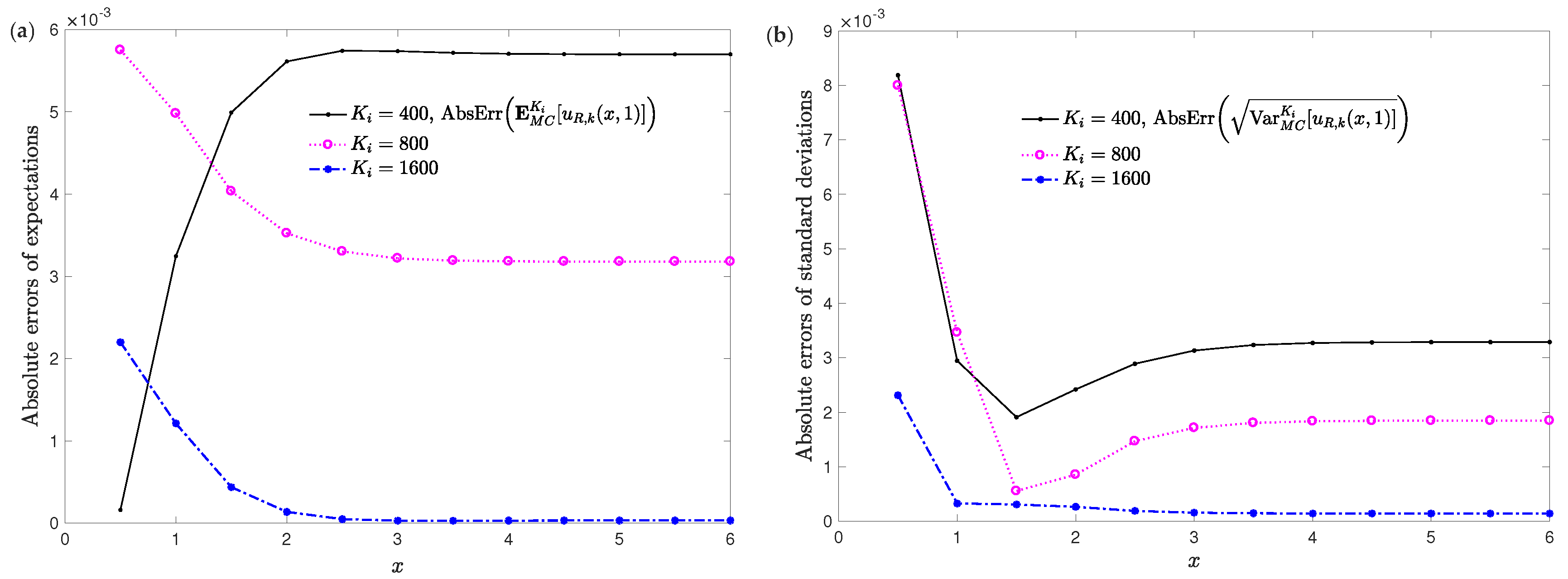
Secondly, by varying the length of the step-size of the trapezoidal quadrature, k , 1 5 , for both R and the number of realized events K fixed, the computed RMSEs are shown in Table 2. Finally, in the last experiment, we have taken several number of realizations K i in the Monte Carlo method checking the improvement of the approaches obtained for both the expectation and the standard deviation; see Table 3. It is observed that for a number of events K equal to 1600 the results are enough precise. In this sense, Figure 2 illustrates the decreasing trend of the absolute errors for both statistical moments when the number of simulations increase.

4.2. Example 2

Let us consider the random parabolic models (1)–(5) with the following choice of data
p ( x ) = 1 1 + a x 2 , q ( x ) = 1 b sin ( x ) , Φ ( x , t ) = e t ,
f 1 ( t ) = 0 , f 2 ( t ) = 2 e t t π , g ( x ) = 0 .
In (51) the r.v. a has a Gaussian distribution of mean μ = 0.1 and standard deviation σ = 0.02 truncated on the interval [ 0.08 , 0.12 ] , a N [ 0.08 , 0.12 ] ( 0.1 ; 0.02 ) , and b follows a gamma distribution of parameters ( 0.8 ; 0.25 ) truncated on the interval [ 0.16 , 0.24 ] , b G a m m a [ 0.16 , 0.24 ] [ 0.8 ; 0.25 ] . Both a and b are considered independent r.v’s. For the choice of data (51) and (52), the listed conditions in Algorithm 1 are satisfied, then we can compute approximations to the statistical moments of the s.p. solution of problem (1)–(5), (51) and (52). In order to evidence the convergence of approximations we will compute the root mean square deviations (RMSDs) for consecutive approximations of the mean and the standard deviation, in two stages. Firstly, varying the length of truncation end-point R by means the following expressions
RMSD E MC K [ u R R + 1 , k ( x i , t ) ] = 1 n i = 1 n E MC K [ u R + 1 , k ( x i , t ) ] E MC K [ u R , k ( x i , t ) ] 2 ,
RMSD Var MC K [ u R R + 1 , k ( x i , t ) ] = 1 n i = 1 n Var MC K [ u R + 1 , k ( x i , t ) ] Var MC K [ u R , k ( x i , t ) ] 2
and secondly, varying the step-size k of the trapezoidal quadrature by means
RMSD E MC K [ u R , k k + 1 ( x i , t ) ] = 1 n i = 1 n E MC K [ u R , k + 1 ( x i , t ) ] E MC K [ u R , k ( x i , t ) ] 2 ,
RMSD Var MC K [ u R , k k + 1 ( x i , t ) ] = 1 n i = 1 n Var MC K [ u R , k + 1 ( x i , t ) ] Var MC K [ u R , k ( x i , t ) ] 2
in the spatial domain [ 0.1 , 1.5 ] for n = 15 points x i = i h , 1 i n , h = Δ x = 0.1 . Table 4 collects the RMSDs (53) and (54) taking k = 0.5 and the number of realized events K fixed (1600). The choice of the values for both parameter k and K are motived by the good results obtained in Example 1. Figure 3 and Figure 4a show the convergence of the approximations for the expectation (35) and the standard deviation (36) as R increases. This behaviour is depicted in Figure 3 and Figure 4b where it is shown the decreasing trend of the absolute deviations (AbsDev) for the expectation and the standard deviation, defined as follows
AbsDev E MC K [ u R R + 1 , k ( x i , t ) = E MC K [ u R + 1 , k ( x i , t ) E MC K [ u R , k ( x i , t ) ,
AbsDev Var [ u R , R + 1 , k ( x i , t ) = Var MC K [ u R + 1 , k ( x i , t ) ] Var MC K [ u R , k ( x i , t ) ] .
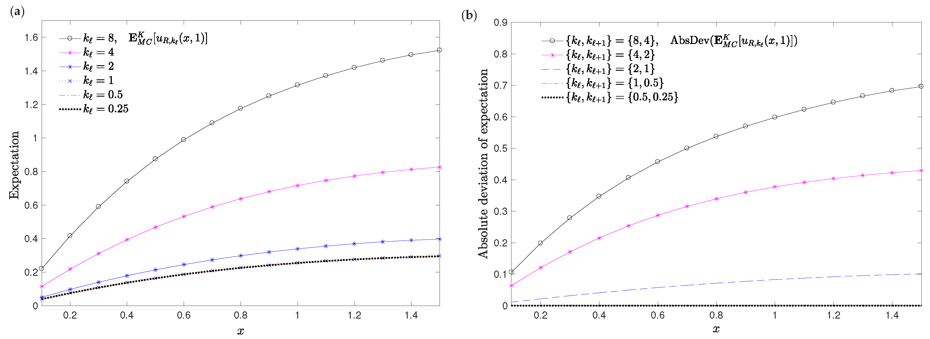
Computations have been carried out by Mathematica© software version 11.3.0.0 for Windows 10Pro (64-bit) AMD Ryzen Threadripper 2990WX 32-Core Processor, 3.00 GHz. As regards the study of the convergence of the approximations for both the expectation and the standard deviation when parameter k changes, Table 5 collects the RMSDs (55) and (56) taking R = 32 and the number of realized events K fixed (1600). The decreasing behaviour of these RMSDs is in full agreement with the results shown in Figure 5 and Figure 6 where it is illustrated how the successive approximations of the absolute deviations for both the expectation and the standard deviation are close to each other when k decreases.
In Table 6 and Table 7 we show the timings (CPU time spent in the Wolfram Language kernel) to compute both statistical moments of the approximated solution (32) plotted in Figure 3, Figure 4, Figure 5 and Figure 6a.

5. Conclusions

In this paper, we focus in the numerical approximation of the solution s.p. and its statistical moments of random heterogeneous parabolic partial differential models following the mean square approach. Random integral transform method is used avoiding iterative methods that are not useful because of the complex nature of the random problem. For the computation of the integrals arising when the random inverse integral transform is applied, we choose non Gaussian quadrature methods instead of the common used Gaussian quadrature ones due to the high oscillatory nature of the involved integrands. Simulations are performed using Monte Carlo method. Illustrative examples show the convergence of the proposed method and the sensibility of the approximate expectation and standard deviation to the number of the realizations considered.

Author Contributions

These authors contributed equally to this work. All authors have read and agreed to the published version of the manuscript.

Funding

This work has been supported by the Spanish Ministerio de Economía, Industria y Competitividad (MINECO), the Agencia Estatal de Investigación (AEI) and Fondo Europeo de Desarrollo Regional (FEDER UE) grant MTM2017-89664-P.

Conflicts of Interest

The authors declare no conflict of interest.

References

  1. Bharucha-Reid, A.T. On the Theory of Random Equations, Stochastic Processes in Mathematical Physics and Engineering. In Proceedings of Symposia in Applied Mathematics, American Mathematical Society XVI; American Mathematical Society: Providence, RI, USA, 1964; pp. 40–69. [Google Scholar]
  2. Bharucha-Reid, A.T. Probabilistic Methods in Applied Mathematics; Academic Press, Inc.: New York, NY, USA, 1973. [Google Scholar]
  3. Bäck, J.; Nobile, F.; Tamellini, L.; Tempone, R. Stochastic Spectral Galerkin and Collocation Methods for PDEs with Random Coefficients: A Numerical Comparison. In Spectral and High Order Methods for Partial Differential Equations. Lecture Notes in Computational Science and Engineering; Hesthaven, J., Rønquist, E., Eds.; Springer: Berlin/Heidelberg, Germany, 2011; Volume 76, pp. 43–62. [Google Scholar]
  4. Ernst, O.; Sprungk, B.; Tamellini, L. Convergence of Sparse Collocation for Functions of Countably Many Gaussian Random Variables (with Application to Elliptic PDEs). SIAM J. Numer. Anal. 2018, 56, 877–905. [Google Scholar] [CrossRef] [Green Version]
  5. Casabán, M.-C.; Cortés, J.-C.; Jódar, L. Analytic-Numerical Solution of Random Parabolic Models: A Mean Square Fourier Transform Approach. Math. Model. Anal. 2018, 23, 79–100. [Google Scholar] [CrossRef]
  6. Casabán, M.-C.; Company, R.; Jódar, L. Numerical Integral Transform Methods for Random Hyperbolic Models with a Finite Degree of Randomness. Mathematics 2019, 7, 853. [Google Scholar] [CrossRef] [Green Version]
  7. Nouri, K.; Ranjbar, H. Mean Square Convergence of the Numerical Solution of Random Differential Equations. Mediterr. J. Math. 2015, 12, 1123–1140. [Google Scholar] [CrossRef]
  8. Casabán, M.-C.; Cortés, J.-C.; Jódar, L. A random Laplace transform method for solving random mixed parabolic differential problems. Appl. Math. Comput. 2015, 259, 654–667. [Google Scholar] [CrossRef]
  9. Iserles, A. On the numerical quadrature of highly oscillating integrals I: Fourier transforms. IMA J. Numer. Anal. 2004, 24, 365–391. [Google Scholar] [CrossRef]
  10. Davis, P.J.; Rabinowitz, P. Methods of Numerical Integration; Academic Press: Orlando, FL, USA, 1984. [Google Scholar]
  11. Casabán, M.-C.; Company, R.; Egorova, V.N.; Jódar, L. Integral transform solution of random coupled parabolic partial differential models. Math. Method Appl. Sci. 2020. [Google Scholar] [CrossRef]
  12. Farlow, S.J. Partial Differential Equations for Scientists and Engineers; Dover: New York, NY, USA, 1993. [Google Scholar]
  13. Jódar, L.; Pérez, J. Analytic numerical solutions with a priori error bounds of initial value problems for the time dependent coefficient wave equation. Util. Math. 2002, 62, 95–115. [Google Scholar]
  14. Soong, T.T. Random Differential Equations in Science and Engineering; Academic Press: New York, NY, USA, 1973. [Google Scholar]
  15. Özişik, M.N. Boundary Value Problems of Heat Conduction; Dover Publications, Inc.: New York, NY, USA, 1968. [Google Scholar]
  16. Polyanin, A.D.; Nazaikinskii, V.E. Handbook of Linear Partial Differential Equations for Engineers and Scientists, 2nd ed.; Taylor & Francis Group: Boca Raton, FL, USA, 2016. [Google Scholar]
  17. Casabán, M.-C.; Company, R.; Cortés, J.-C.; Jódar, L. Solving the random diffusion model in an infinite medium: A mean square approach. Appl. Math. Model. 2014, 38, 5922–5933. [Google Scholar] [CrossRef]
  18. Casabán, M.-C.; Cortés, J.-C.; Jódar, L. Solving linear and quadratic random matrix differential equations using: A mean square approach. The non-autonomous case. J. Comput. Appl. Math 2018, 330, 937–954. [Google Scholar] [CrossRef]
  19. Davies, B.; Martin, B. Numerical Inversion of the Laplace Transform: A Survey and Comparison of Methods. J. Comput. Phys. 1979, 33, 1–32. [Google Scholar] [CrossRef]
  20. Cohen, A.M. Numerical Methods for Laplace Transform Inversion; Springer: New York, NY, USA, 2007. [Google Scholar]
  21. Kroese, D.P.; Taimre, T.; Botev, Z.I. Handbook of Monte Carlo Methods; Wiley Series in Probability and Statistics; John Wiley & Sons: New York, NY, USA, 2011. [Google Scholar]
  22. Asmussen, S.; Glynn, P.W. Stochastic Simulation: Algorithms and Analysis; Springer Science & Business Media: Berlin/Heidelberg, Germany, 2007; Volume 57. [Google Scholar]
  23. Ng, E.W.; Geller, M. A Table of Integrals of the Error Functions. Natianal Bur. Stand.-B Math. Sci. 1969, 73B, 1–20. [Google Scholar] [CrossRef]
  24. Abramowitz, M.; Stegun, I.A. Handbook of Mathematical Functions with Formulas, Graphs, and Mathematical Tables; Dover Publications, Inc.: New York, NY, USA, 1972. [Google Scholar]
  25. Armstrong, J.S.; Collopy, F. Error measures for generalizing about forecasting methods: Empirical comparisons. Int. J. Forecast. 1992, 8, 69–80. [Google Scholar] [CrossRef] [Green Version]
  26. Mathematica, Version 11.3; Wolfram Research, Inc.: Champaign, IL, USA, 2018.
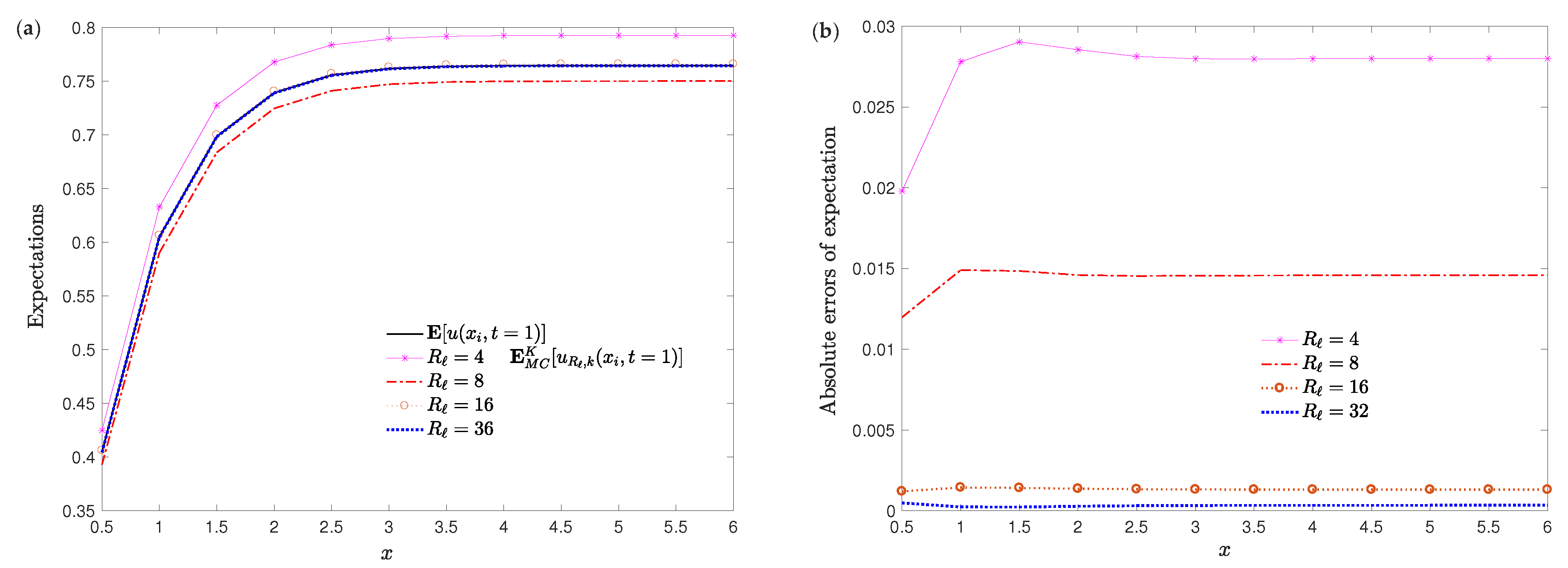
Figure 1. Example 1. (a) Expectation of the exact solution (38) and (39) considering a 0 = a and b 0 = b as the r.v.’s taken in this Example 1 versus approximations of the expectation (35), (47) and (48) for several lengths of the truncation end-point R. (b) Absolute errors of expectations for several values of R. For both left and right t = 1 , k = 0.2 , K = 5000 and R { 4 , 8 , 16 , 32 } . The spatial domain considered is x i [ 0.5 , 6 ] with x i = i h , h = 0.5 .
Mathematics 08 01112 g001
Figure 2. Example 1.(a) Absolute errors of the expectation for (47) and (48). (b) Absolute errors of standard deviation for (47) and (48). For both left and right, t = 1 , k = 0.2 , R = 16 and K i { 400 , 800 , 1600 } . The spatial domain considered is x i [ 0.5 , 6 ] with x i = i h , h = 0.5 .
Mathematics 08 01112 g002
Figure 3. Example 2. (a) Expectations computed by (35). (b) Absolute deviations of the expectations computed by (57). For both left and right, the parameters t = 1 , k = 0.5 , α = 0.5 , K = 1600 are fixed while the length of the truncation end-point R changes, R { 2 , 3 , 4 , 5 , 6 , 7 } . The spatial domain is x [ 0.1 , 1.5 ] with Δ x = 0.1 .
Mathematics 08 01112 g003
Figure 4. Example 2. (a) Standard deviations computed by (36). (b) Absolute deviations of the standard deviations computed by (58). For both left and right, the parameters t = 1 , k = 0.5 , α = 0.5 , K = 1600 are fixed while the length of the truncation end-point R changes, R { 2 , 4 , 8 , 16 , 32 , 64 } . The spatial domain is x [ 0.1 , 1.5 ] with Δ x = 0.1 .
Mathematics 08 01112 g004
Figure 5. Example 2. (a) Expectations computed by (35). (b) Absolute deviations of the expectations computed by (57). For both left and right, the parameters t = 1 , R = 32 , α = 0.5 , K = 1600 are fixed while step-size of the trapezoidal quadrature k changes, k { 8 , 4 , 2 , 1 , 0.5 , 0.25 } . The spatial domain is x [ 0.1 , 1.5 ] with Δ x = 0.1 .
Mathematics 08 01112 g005
Figure 6. Example 2. (a) Standard deviations computed by (36). (b) Absolute deviations of the standard deviations computed by (58). For both left and right, the parameters t = 1 , R = 32 , α = 0.5 , K = 1600 are fixed while the step-size of the trapezoidal quadrature k changes, k { 8 , 4 , 2 , 1 , 0.5 , 0.25 } . The spatial domain is x [ 0.1 , 1.5 ] with Δ x = 0.1 .
Mathematics 08 01112 g006
Table 1. Example 1. Root mean square errors (RMSEs) for the expectation (49) and the standard deviation (50) considering the discretization on the spatial domain [ 0.5 , 6 ] in the following way x i = i h , 1 i 12 , h = Δ x = 0.2 , taking fixed α = 0.5 , K = 5000 simulations and k = 0.2 but varying the length of the truncation end-point R { 4 , 8 , 16 , 32 } at the temporal instant t = 1 .
R RMSE E MC K [ u R , k ( x i , 1 ) ] CPU,sRMSE Var MC K [ u R , k ( x i , 1 ) ] CPU,s
42.75343 × 10 2 14.8438 4.21989 × 10 4 7.1250
81.44244 × 10 2 28.6094 7.36449 × 10 4 25.0469
161.33445 × 10 3 58.1719 4.23940 × 10 4 107.2660
323.36898 × 10 4 175.6090 4.27797 × 10 4 495.0470
Table 2. Example 1. RMSEs for the expectation (49) and the standard deviation (50) considering the discretization on the spatial domain [ 0.5 , 6 ] in the following way x i = i h , 1 i 12 , h = Δ x = 0.2 , taking fixed α = 0.5 , K = 5000 simulations and R = 16 but varying the step-size of the trapezoidal quadrature k { 0.8 , 0.4 , 0.2 , 0.1 , 0.05 } at the temporal instant t = 1 .
k RMSE E MC K [ u R , k ( x i , 1 ) ] CPU,sRMSE Var MC K [ u R , k ( x i , 1 ) ] CPU,s
0.8 1.28377 × 10 4.6719 4.75391× 10 2 7.2344
0.4 4.23282 × 10 3 8.4375 9.02170 × 10 4 31.5625
0.2 1.33445 × 10 3 57.6094 4.23940 × 10 4 135.9220
0.1 1.14283 × 10 3 115.3280 4.25683 × 10 4 601.5940
0.05 1.04648 × 10 3 270.3590 4.26453 × 10 4 2315.3000
Table 3. Example 1. RMSEs of the expectation (49) and the standard deviation (50) for the solution s.p. (47) and (48) at t = 1 in x [ 0.5 , 6 ] with Δ x = 0.5 varying the number of realizations K i for R = 16 and k = 0.2 ( M = 80 ).
K i RMSE E MC K [ u R , k ( x , 1 ) ] CPU, sRMSE Var MC K [ u R , k ( x , 1 ) ] CPU, s
1002.16541 × 10 3 1.2813 2.97642 × 10 3 4.9531
2001.19892 × 10 3 2.3750 5.94483 × 10 4 6.2656
4005.22902 × 10 3 6.4375 3.73953 × 10 3 10.2031
8003.74892 × 10 3 9.0000 2.92100 × 10 3 16.2031
16007.37703 × 10 4 17.9063 6.96690 × 10 4 27.9063
32007.94225 × 10 4 38.8750 7.89259 × 10 4 60.4688
Table 4. Example 2. RMSDs at t = 1 for the expectation (53) and the standard deviation (54) considering the discretization on the spatial domain [ 0.1 , 1.5 ] in the following way x i = i h , 1 i 15 , h = Δ x = 0.1 , taking K = 1600 simulations and k = 0.5 both fixed.
{ R , R + 1 } RMSD E MC K [ u R R + 1 , k ( x i , 1 ) ] RMSD Var MC K [ u R R + 1 , k ( x i , 1 ) ]
{ 2 , 4 } 4.08921 × 10 2 2.39328 × 10 4
{ 4 , 8 } 2.72959 × 10 2 2.57692 × 10 4
{ 8 , 16 } 1.03896 × 10 2 8.86479 × 10 5
{ 16 , 32 } 1.61474 × 10 3 3.36047 × 10 5
{ 32 , 64 } 8.11820 × 10 4 2.62627 × 10 5
Table 5. Example 2. RMSDs at t = 1 for the expectation (55) and the standard deviation (56) considering the discretization on the spatial domain [ 0.1 , 1.5 ] in the following way x i = i h , 1 i 15 , h = Δ x = 0.1 , taking K = 1600 simulations and R = 32 .
{ k , k + 1 } RMSD E MC K [ u R , k k + 1 ( x i , 1 ) ] RMSD Var MC K [ u R , k k + 1 ( x i , 1 ) ]
{ 8 , 4 } 5.18967 × 102.57413 × 10 3
{ 4 , 2 } 3.24473 × 101.88253 × 10 3
{ 2 , 1 } 7.14500 × 10 2 8.83031 × 10 5
{ 1 , 0.5 } 1.03254 × 10 3 3.25342 × 10 5
{ 0.5 , 0.25 } 6.92989 × 10 4 2.62627 × 10 5
Table 6. Example 2. CPU time spent to compute the approximations of the expectation (35) and the standard deviation (36) of (47) and (48) considering the discretization on the spatial domain [ 0.1 , 1.5 ] in the following way x i = i h , 1 i 15 , h = Δ x = 0.1 , taking K = 1600 simulations and k = 0.5 at the temporal instant t = 1 .
R CPU,s E MC K [ u R , k ( x i , 1 ) ] CPU,s Var MC K [ u R , k ( x i , 1 ) ]
2 24.375 25.2188
4 46.9688 45.9375
8 58.6875 75.5000
16 102.6250 143.109
32 219.5780 209.3280
64 359.7190 253.5000
Table 7. Example 2. CPU time spent to compute the expectation (35) and the standard deviation (36) of (47) and (48) considering the discretization on the spatial domain [ 0.1 , 1.5 ] in the following way x i = i h , 1 i 15 , h = Δ x = 0.1 , taking K = 1600 simulations and R = 32 at the temporal instant t = 1 .
k CPU,s E MC K [ u R , k ( x i , 1 ) ] CPU,s Var MC K [ u R , k ( x i , 1 ) ]
8 13.8438 13.3750
4 24.1563 22.9219
2 44.7656 43.8438
1 88.9844 119.6410
0.5 165.0000 239.1250
0.25 351.0000 362.5630