A Method for Assessing Regional Bioenergy Potentials Based on GIS Data and a Dynamic Yield Simulation Model


Abstract
:1. Introduction
2. Materials and Methods
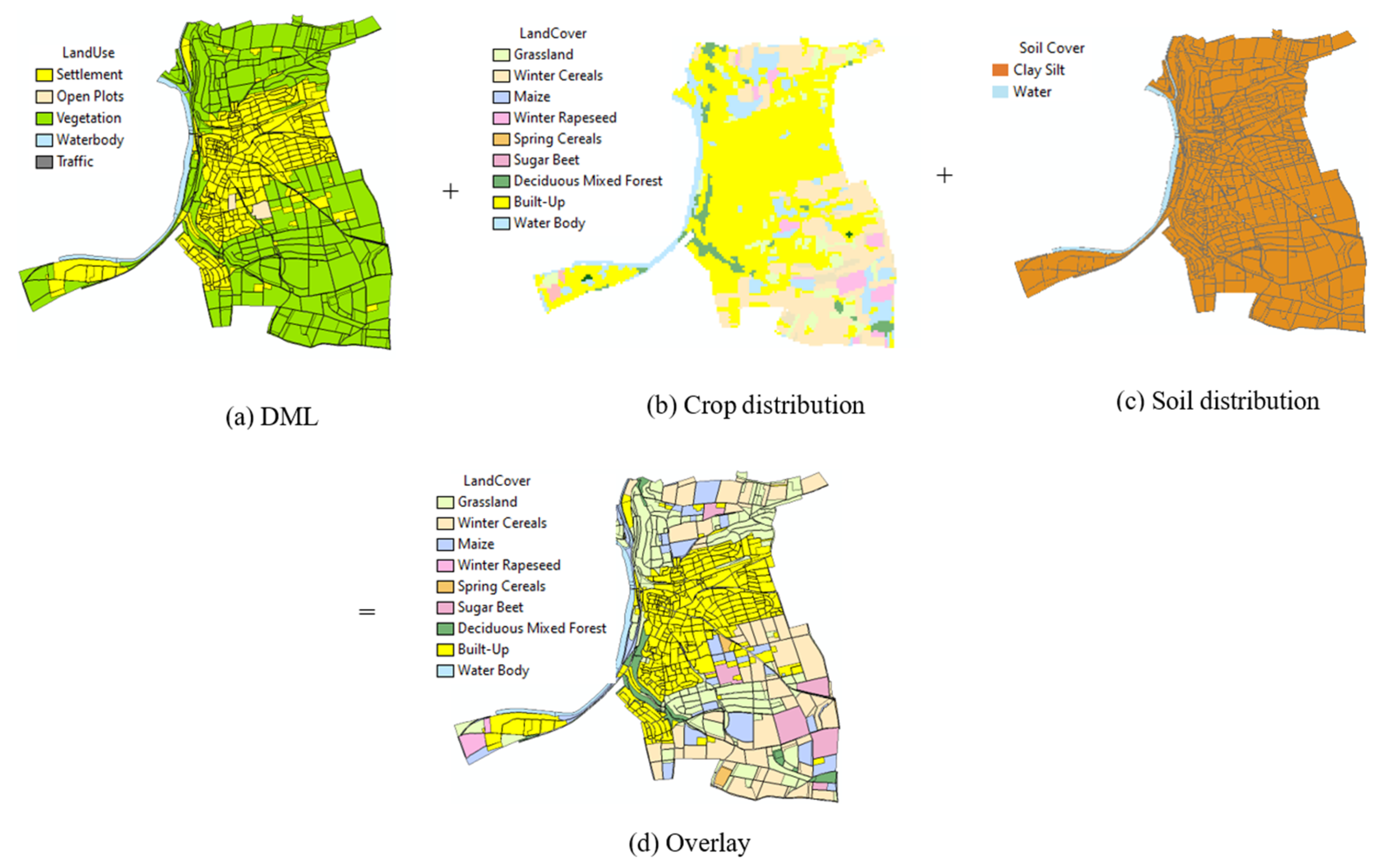
2.1. Input Data
2.2. Assessment Method for Local Biomass Potential
2.3. Dynamic Yield Model
2.4. Calculation of Bioenergy Potentials
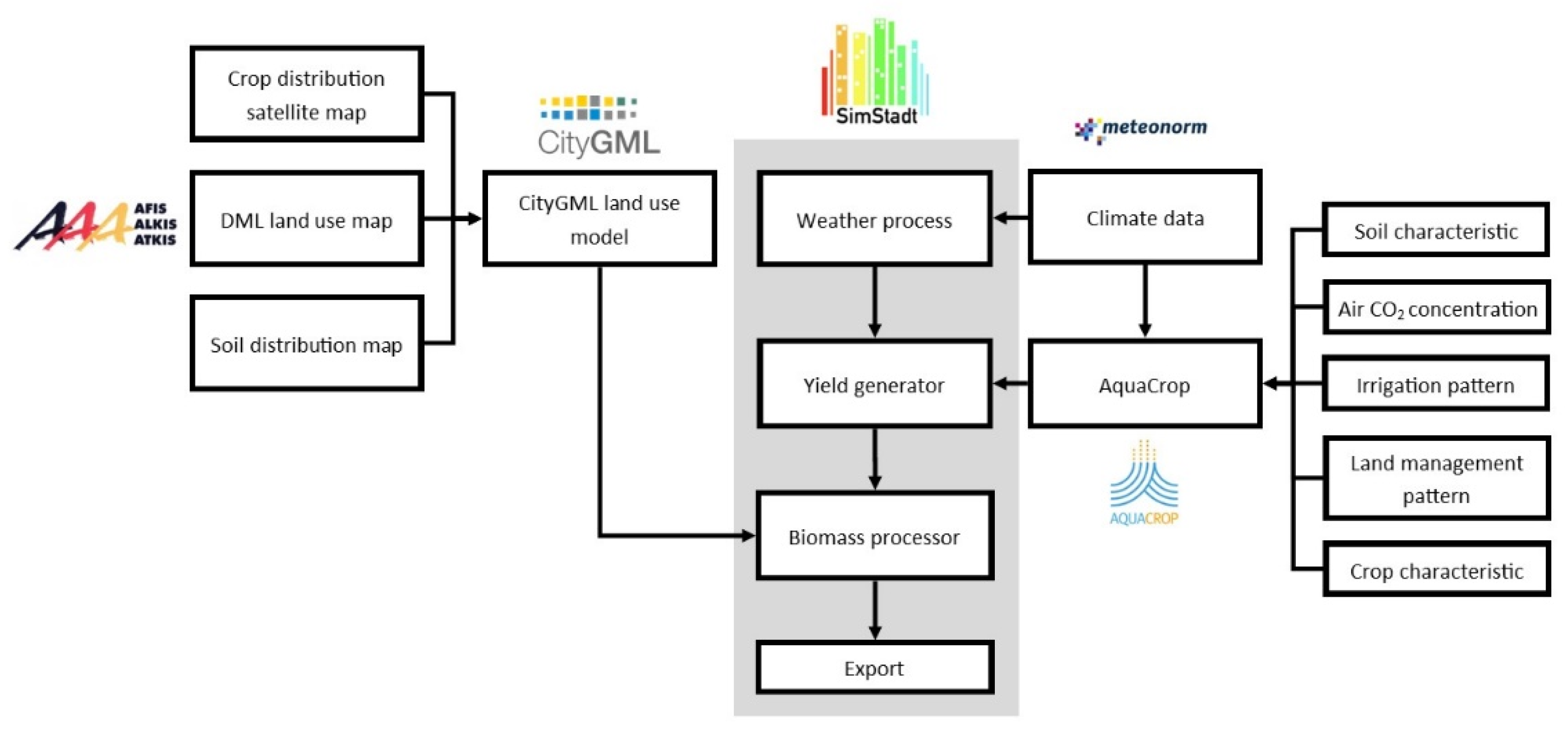
2.5. Simulation Environment and Interface
2.6. Approach to Data Validation
2.7. Scenarios Setting
2.8. Ludwigsburg and Dithmarschen Test Cases
3. Results
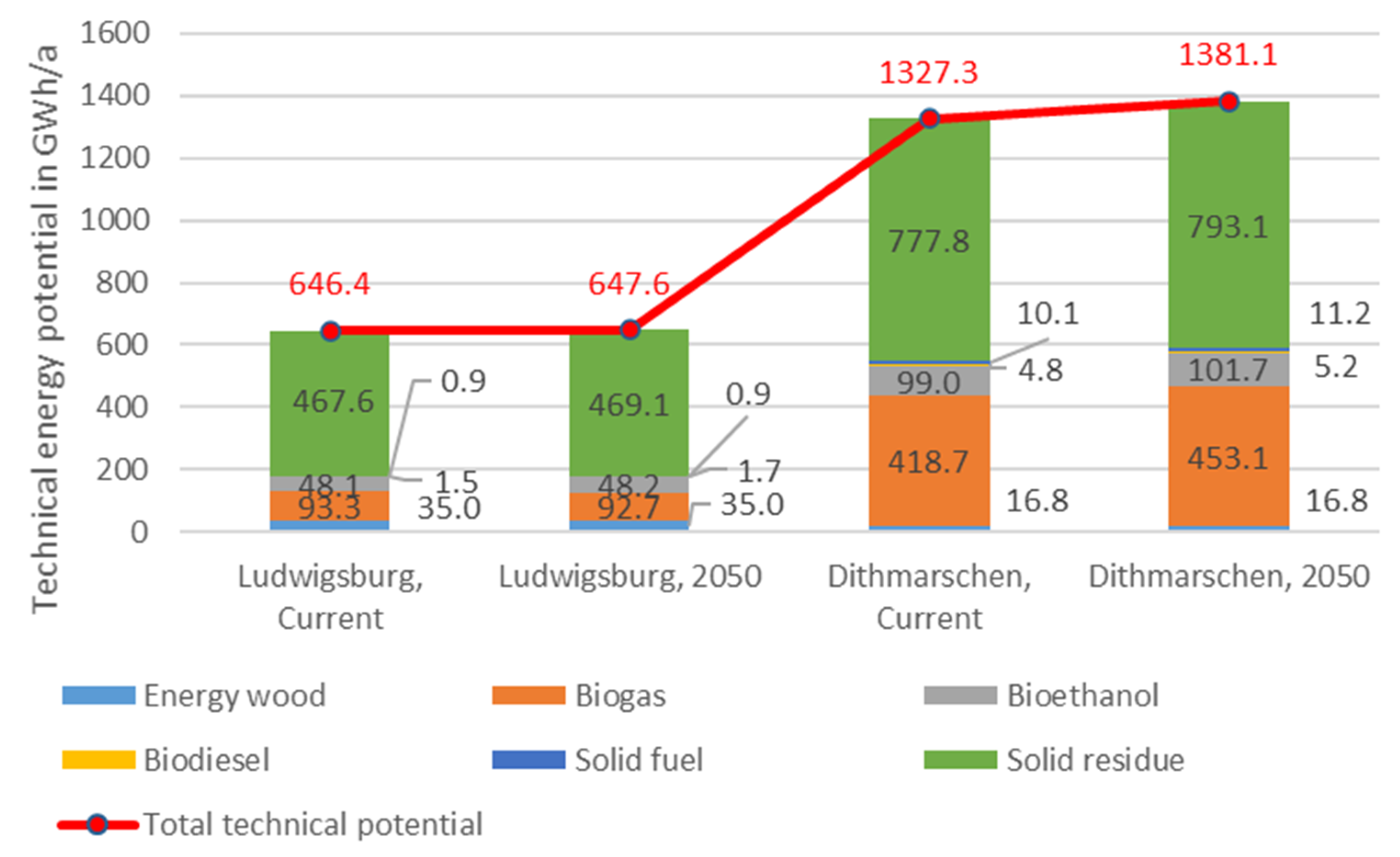
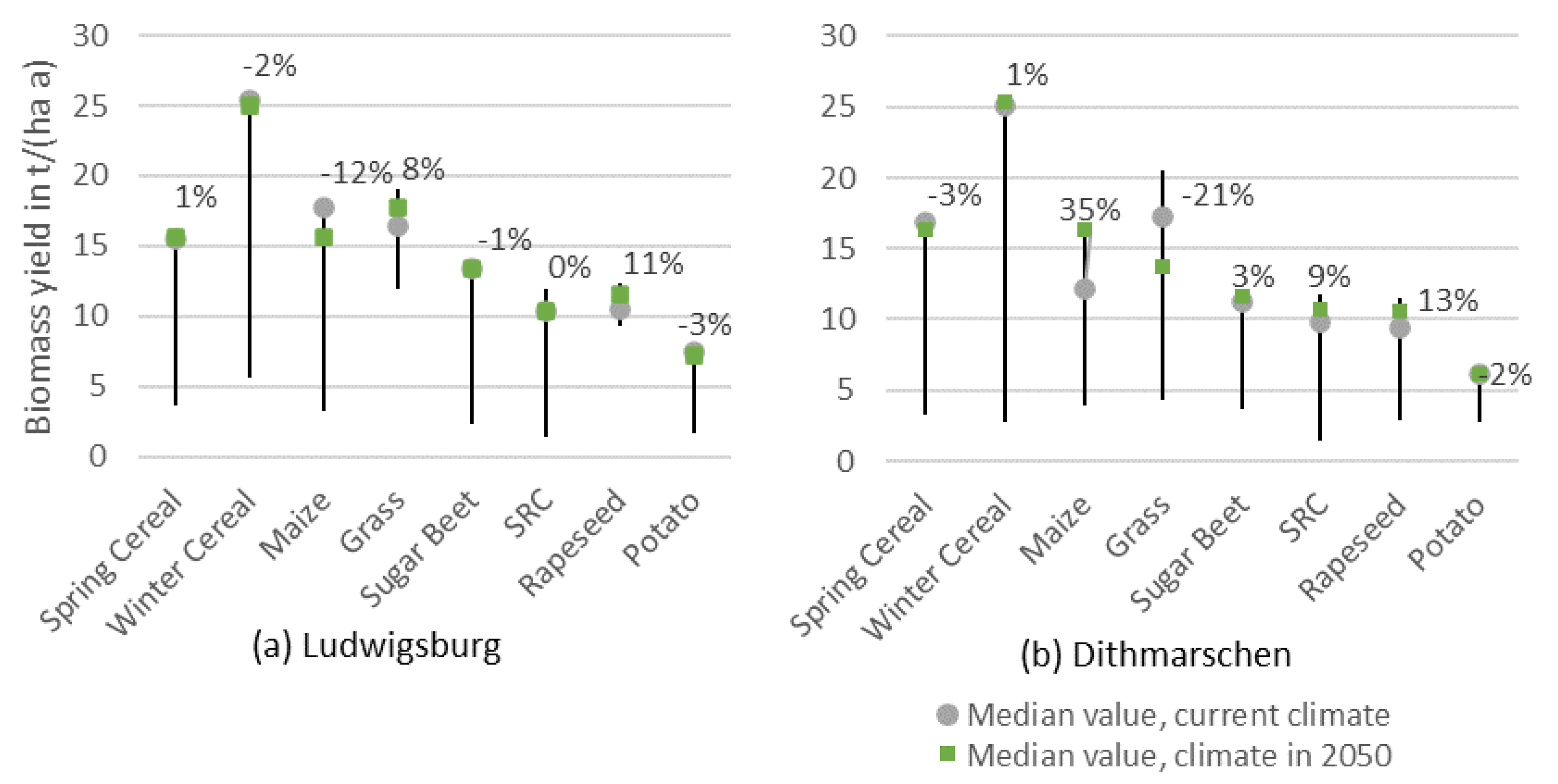
3.1. The Impact of Climate Change
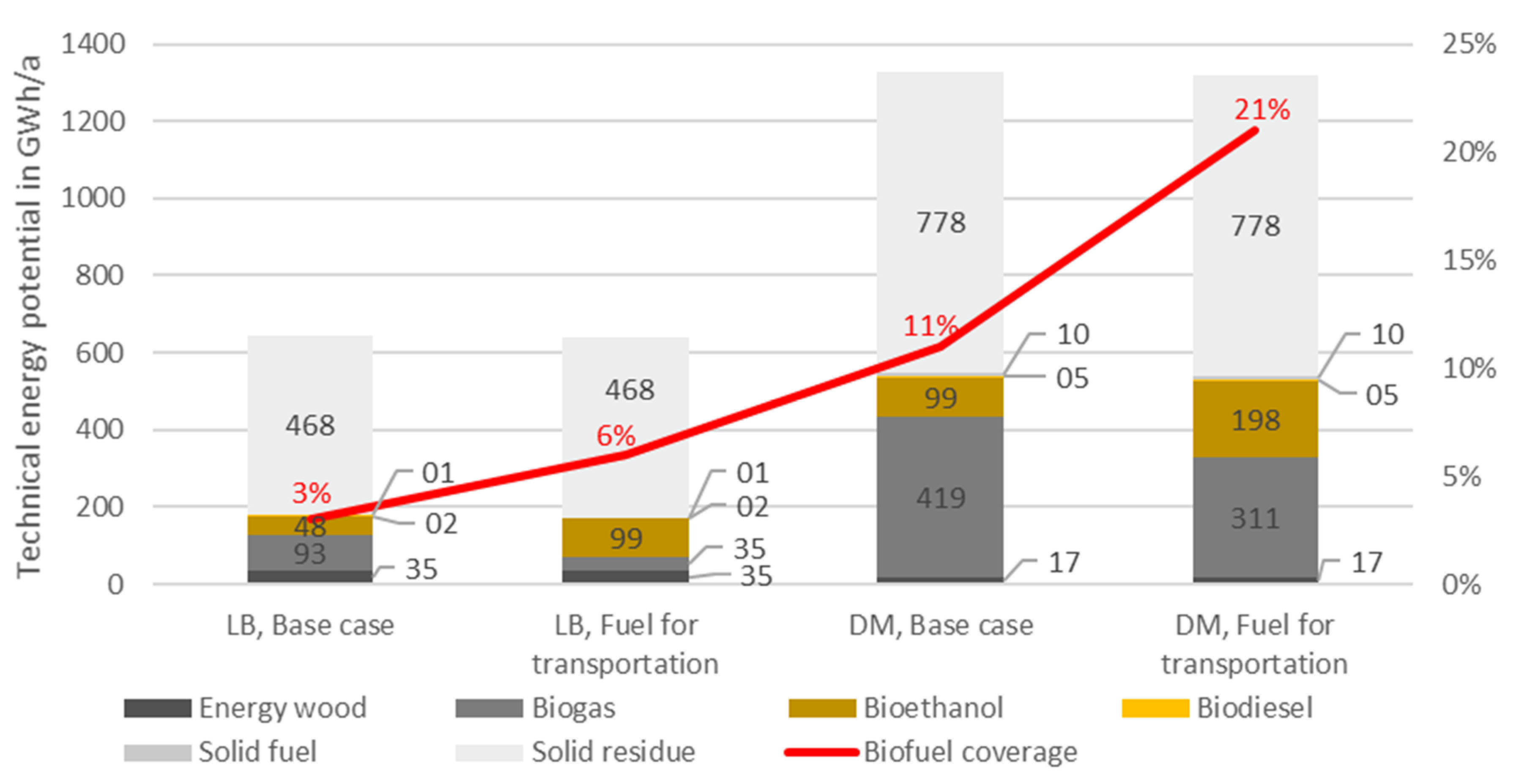
3.2. Optimizing Biofuel for Tranportation Sector
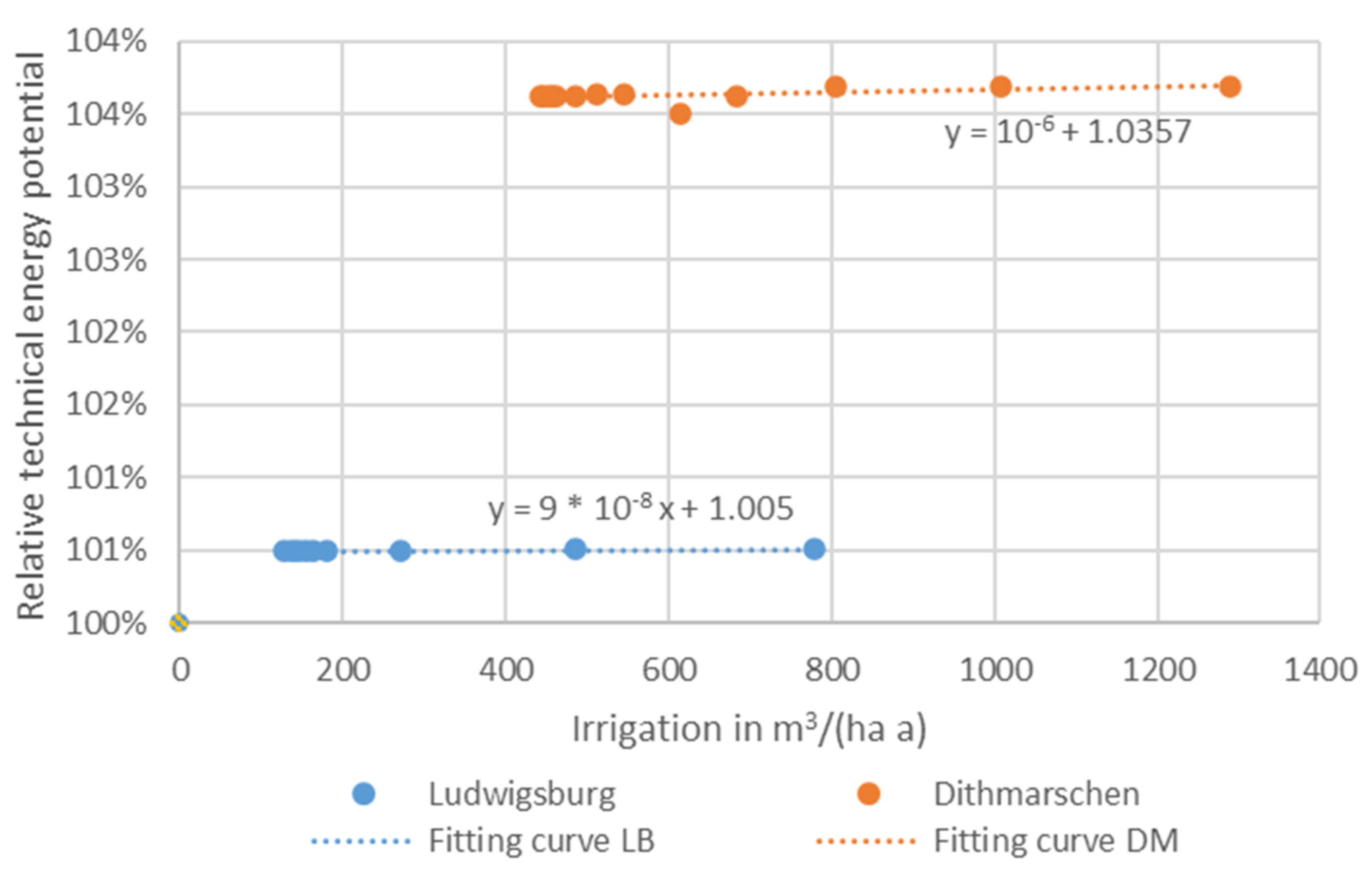
3.3. The Impact of Irrigation
4. Discussion
5. Conclusions
Author Contributions
Funding
Acknowledgments
Conflicts of Interest
Abbreviations
| Abbreviations | Explanation |
| GIS | Geographic information system |
| RES | Renewable energy sources |
| FWE | Food-Water-Energy |
| DLM | Digital Landscape Model |
| ALKIS | Germany’s Official Real Property Cadastre Information System |
| AdV | Working Group of the Surveying Authorities of the sixteen states of Germany |
| KA5 | German soil classification system |
| SRC | Short Rotation Coppice |
| ΣTr | Crop transpiration |
| WP | Water productivity |
| WP* | Normalized water productivity |
| CO2 | Carbon dioxide |
| RAW | Readily Available Water |
| CityGML | City Geography Markup Language |
| FAO | Food and Agriculture Organization of the United Nations |
| ETo | Crop reference evapotranspiration |
| XML | Extensible Markup Language |
| GYGA | Global Yield Gap Atlas |
| DM | Dry mass |
| RED II | Renewable Energy Directive 2018/2001 |
| LB | County Ludwigsburg |
| DM | County Dithmarschen |
| PV | Photovoltaic |
Appendix A

| Soil Surface not Sealed | Soil Surface Sealed |
|---|---|
| Pure sands | City center areas (surface > 70 % sealed) |
| Silty sands | |
| Normal clays | Anthropogenically embossed surfaces (surface 30–70% sealed) |
| Loamy silt | |
| Silt clays | Technogenic ally designed areas, including mining areas |
| Loamy sands | |
| Sand Loams | |
| Clay Loams | |
| Clay silt | |
| Moors | |
| Tidal flats |
Appendix B
| Potential | Parameter | Unit | Winter Cereal | Spring Cereal | Maize | Grass |
| Theoretical potential | Wet mass range 6 | t/ha a | 9.5–20 | 8.0–17 | 10.0–22.0 | 9.0–18.8 |
| Water content 6 | % | 15 | 15 | 67 | 15 | |
| Heating value 4,5,8 | MJ/kg | 17.1 | 17.1 | 17.1 | 16.5 | |
| Primary biomass yield factor | GJ/(ha t ha) | 14.5 | 14.5 | 5.6 | 14.0 | |
| Biogas | oTS Organic dry mass of dry mass 7 | % | 94 | 95 | 95 | 88 |
| Biogas yield 7 | l_N/kg oTS | 520 | 520 | 600 | 560 | |
| Methan content 7,8 | % | 52.0 | 52.0 | 52.0 | 54.0 | |
| biogas coefficient per fresh mass yield | GJ/(t FM ha a) | 7.8 | 7.9 | 3.5 | 8.1 | |
| Bioethanol | Conversion efficiency 3 | GJ/GJ_Primary | 0.5 | 0.5 | 0.4 | - |
| Biodiesel | Conversion efficiency 3 | GJ/GJ_Primary | ||||
| Residue | Yield range 1,2 | t FM/(ha a) | 3.5–9.4 | 3.5–9.4 | 4.2–10 | 4.2–26 |
| Residue yield factor | t_residue FM/ t_biomass FM | 0.4 | 0.4 | 0.4 | 1.0 | |
| Water content | % | 14 | 14 | 14 | 50 | |
| Heat value | GJ/kg | 0.0143 | 0.0143 | 0.0143 | 0.0143 | |
| Residue factor | GJ/t FM biomass | 5.2 | 5.5 | 5.0 | 7.2 | |
| Potential | Parameter | Unit | Sugar Beet | SRC | Rapeseed | Potato |
| Theoretical potential | Wet mass range 6 | t/ha a | 40–85 | 4–18 | 8.5–13.5 | 33–50 |
| Water content 6 | % | 76 | 29 | 12 | 76 | |
| Heating value 4,5,8 | MJ/kg | 17.4 | 18.5 | 18.0 | 18.0 | |
| Primary biomass yield factor | GJ/(ha t ha) | 4.2 | 13.1 | 15.8 | 4.3 | |
| Biogas | oTS Organic dry mass of dry mass 7 | % | 92 | 91 | 85 | 90 |
| Biogas yield 7 | l_N/kg oTS | 700 | 516 | 630 | 640 | |
| Methan content 7,8 | % | 51 | 52.2 | 55.3 | 50 | |
| biogas coefficient per fresh mass yield | GJ/(t FM ha a) | 2.8 | 6.3 | 9.4 | 2.5 | |
| Bioethanol | Conversion efficiency 3 | GJ/GJ_Primary | 0.8 | 0.4 | - | 0.6 |
| Biodiesel | Conversion efficiency 3 | GJ/GJ_Primary | - | - | 0.3 | - |
| Residue | Yield range 1,2 | t FM/(ha a) | 10.0–32.0 | 2.5–4 | 4.2–10 | 10–32 |
| Residue yield factor | t_residue FM/ t_biomass FM | 0.3 | 0.3 | 0.6 | 0.5 | |
| Water content | % | 66 | 66 | 14 | 66 | |
| Heat value | GJ/kg | 0.0143 | 0.0143 | 0.0143 | 0.0143 | |
| Residue factor | GJ/t FM biomass | 1.5 | 1.6 | 7.3 | 2.3 |
Appendix C
| Parameter | Winter Cereal | Spring Cereal | Maize | Sugar Beet | Potato | SRC |
|---|---|---|---|---|---|---|
| Base temperature °C | 5 | 0 | 8 | 5 | 2 | 0 |
| Upper temperature °C | 35 | 26 | 30 | 30 | 26 | 25 |
| Plant density (Plants per ha) | 2,000,000 | 4,500,000 | 75,000 | 100,000 | 40,000 | 266,667 |
| Plant to emergence (GDD) | 88 | 150 | 80 | 23 | 200 | 0 |
| Planting to maximum rooting depth (GDD) | 720 | 864 | 1409 | 408 | 1079 | 3080 |
| Planting to start senescence (GDD) | 819 | 1700 | 1400 | 1704 | 984 | 2410 |
| Planting to maturity (GDD) | 2162 | 2400 | 1700 | 2203 | 1276 | 3080 |
| Planting to flowering (GDD) | 754 | 1250 | 880 | 865 | 550 | 0 |
| Maximum rooting depth (m) | 1.2 | 1.5 | 2.3 | 1 | 1.5 | 0.8 |
| Maximum canopy cover in fraction soil cover | 0.91 | 0.96 | 0.96 | 0.98 | 0.92 | 0.96 |
| Water productivity normalized for ET0 and CO2 (g/m2) | 15 | 15 | 33.7 | 17 | 18 | 10.4 |
| Canopy growth coefficient (CGC) (fraction soil cover per day) (GDD) | 0.02833 | 0.005001 | 0.012494 | 0.010541 | 0.01615 | 0.003543 |
| Canopy decline coefficient (CDC): decrease in canopy cover (in fraction per day) (GDD) | 0.0668 | 0.004 | 0.01 | 0.003857 | 0.002 | 0.00383 |
| Soil water depletion factor for canopy expansion, upper limit | 0.25 | 0.2 | 0.14 | 0.2 | 0.2 | 0.25 |
| Soil water depletion factor for canopy expansion, lower limit | 0.55 | 0.65 | 0.72 | 0.6 | 0.6 | 0.55 |
| Shape factor for water stress coefficient for canopy expansion | 4 | 5 | 2.9 | 3 | 3 | 0 |
| Soil water depletion factor for pollination (p-pol), upper threshold | 0.9 | 0.85 | 0.8 | 0.8 | 0.8 | 0.9 |
| Shape factor for water stress coefficient for stomatal closure | 3 | 2.5 | 6 | 3 | 3 | 0 |
| Shape factor for water stress coefficient for canopy senescence | 3 | 2.5 | 2.7 | 3 | 3 | 0 |
| Parameter | Winter Cereal | Spring Cereal |
|---|---|---|
| Base temperature °C | 5 | 0 |
| Upper temperature °C | 30 | 30 |
| Plant density (Plants per ha) | 60,000 | 440,000 |
| Plant to emergence (Calendar Days) | 11 | 7 |
| Planting to maximum rooting depth (Calendar Days) | 124 | 70 |
| Planting to start senescence (Calendar Days) | 209 | 120 |
| Planting to maturity (Calendar Days) | 244 | 206 |
| Planting to flowering (Calendar Days) | 0 | 87 |
| Maximum rooting depth (m) | 0.7 | 0.3 |
| Maximum canopy cover in fraction soil cover | 0.75 | 0.8 |
| Water productivity normalized for ET0 and CO2 (g/m2) | 14 | 18.6 |
| Canopy growth coefficient (CGC) (fraction soil cover per day) (Calendar Days) | 0.04626 | 0.09713 |
| Canopy decline coefficient (CDC): decrease in canopy cover (in fraction per day) (Calendar Days) | 0.17 | 0.052 |
| Soil water depletion factor for canopy expansion, upper limit | 0 | 0.2 |
| Soil water depletion factor for canopy expansion, lower limit | 0.35 | 0.55 |
| Shape factor for water stress coefficient for canopy expansion | 2.5 | 3.5 |
| Soil water depletion factor for pollination (p-pol), upper threshold | 0.9 | 0.9 |
| Shape factor for water stress coefficient for stomatal closure | 2 | 5 |
| Shape factor for water stress coefficient for canopy senescence | 2 | 3 |
Appendix D
| Parameter | Default Value | Explanation |
|---|---|---|
| Conifer trees harvest rate | 4.5% [23] | The percentage in volume of conifer trees harvested annually out of all conifer trees |
| Deciduous trees harvest rate | 3.0% [23] | The percentage in volume of deciduous trees harvested annually out of all deciduous trees |
| Forest energy usage rate | 25.6% [25] | The percentage in volume of solid forest wood with diameters > 7 cm that is used for energy purposes |
| Energy crop rate | 14.0% [29] | The percentage of farmland area used for energy crop cultivation (e.g., rapeseed, maize). Energy crops are used exclusively for energetic purposes. Since no data source gives information on the end product of a crop (energy or food) per field, we assume, in line with statistical data, that 14% of each field’s area is used for energetic purposes. |
| Residue energy usage rate | 62.0% [30] | The percentage of residue by-products which are used for energetic purposes. |
| Rate of maize residue for Biogas production | 39.4% [29,31] | The percentage of maize residue (silage) for biogas production. The rest of maize residue of maize is used as solid fuel. |
| Crop | Biogas | Bioethanol | Vegetable Oil | Solid Fuel |
|---|---|---|---|---|
| Cereal | 57% | 43% | – | – |
| Maize | – | 100% | – | – |
| Short-rotation coppice (SRC) | – | – | – | 100% |
| Sugar beet | 42% | 58% | – | – |
| Rapeseed | – | – | 100% | – |
| Grass | 98% | – | 0% | 2% |
Appendix E
References
- Scarlat, N.; Dallemand, J.F.; Taylor, N.; Banja, M.; Sanchez Lopez, J.; Avraamides, M. Brief on Biomass for Energy in the European Union; Publications Office of the European Union: Luxembourg, 2019; ISBN 927977235X. [Google Scholar]
- German National Academy of Sciences Leopoldina; acatech—National Academy of Science and Engineering; Union of the German Academies of Sciences and Humanities. Biomass: Striking a Balance between Energy and Climate Policies. Strategies for Sustainable Bioenergy Use; acatech—National Academy of Science and Engineering: Munich, Germany; German National Academy of Sciences Leopoldina: Schweinfurt, Germany; Union of the German Academies of Sciences and Humanities: Munich, Germany, 2019; ISBN 978-3-8047-3929-1. [Google Scholar]
- Berndes, G.; Hoogwijk, M.; van den Broek, R. The contribution of biomass in the future global energy supply: A review of 17 studies. Biomass Bioenergy 2003, 25, 1–28. [Google Scholar] [CrossRef]
- Mittelstädt, A.; Köhler, S.; Sihombing, R.; Duminil, E.; Coors, V.; Eicker, U.; Schröter, B. (Eds.) A Multi-Scale, Web-Based Interface for Strategic Planning of Low-Carbon City Quarters, Proceedings of the Second International Conference on Urban Informatics, Hong Kong, China, 24–26 June 2019; The Hong Kong Polytechnic University: Hong Kong, China, 2019. [Google Scholar]
- Braun, R.; Weiler, V.; Zirak, M.; Dobisch, L.; Coors, V.; Eicker, U. Using 3D CityGML Models for Building Simulation Applications at District Level. In Proceedings of the 2018 IEEE International Conference on Engineering, Technology and Innovation (ICE/ITMC), Stuttgart, Germany, 17–20 June 2018; pp. 1–8. [Google Scholar]
- Bouchard, S.; Landry, M.; Gagnon, Y. Methodology for the large scale assessment of the technical power potential of forest biomass: Application to the province of New Brunswick, Canada. Biomass Bioenergy 2013, 54, 1–17. [Google Scholar] [CrossRef]
- Ericsson, K.; Nilsson, L.J. Assessment of the potential biomass supply in Europe using a resource-focused approach. Biomass Bioenergy 2006, 30, 1–15. [Google Scholar] [CrossRef] [Green Version]
- Lauka, D.; Barisa, A.; Blumberga, D. Assessment of the availability and utilization potential of low-quality biomass in Latvia. Energy Procedia 2018, 147, 518–524. [Google Scholar] [CrossRef]
- Haase, M.; Rösch, C.; Ketzer, D. GIS-based assessment of sustainable crop residue potentials in European regions. Biomass Bioenergy 2016, 86, 156–171. [Google Scholar] [CrossRef]
- Lozano-García, D.F.; Santibañez-Aguilar, J.E.; Lozano, F.J.; Flores-Tlacuahuac, A. GIS-based modeling of residual biomass availability for energy and production in Mexico. Renew. Sustain. Energy Rev. 2020, 120, 109610. [Google Scholar] [CrossRef]
- Quinta-Nova, L.; Fernandez, P.; Pedro, N. GIS-Based Suitability Model for Assessment of Forest Biomass Energy Potential in a Region of Portugal. IOP Conf. Ser. Earth Environ. Sci. 2017, 95, 42059. [Google Scholar] [CrossRef]
- Voivontas, D.; Assimacopoulos, D.; Koukios, E.G. Assessment of biomass potential for power production: A GIS based method. Biomass Bioenergy 2001, 20, 101–112. [Google Scholar] [CrossRef]
- Padsala, R.; Coors, V. Conceptualizing, Managing and Developing: A Web Based 3D City Information Model for Urban Energy Demand Simulation. 2307-8251. 2015. [Google Scholar] [CrossRef]
- Rodríguez, L.R.; Duminil, E.; Ramos, J.S.; Eicker, U. Assessment of the photovoltaic potential at urban level based on 3D city models: A case study and new methodological approach. Solar Energy 2017, 146, 264–275. [Google Scholar] [CrossRef]
- Arbeitsgemeinschaft der Vermessungsverwaltungen der Länder der Bundesrepublik Deutschland. Digitales Basis-Landschaftsmodell (Basis-DLM). Available online: http://www.adv-online.de/AdV-Produkte/Geotopographie/Digitale-Landschaftsmodelle/Basis-DLM/ (accessed on 10 November 2020).
- Griffiths, P.; Nendel, C.; Hostert, P. Intra-annual reflectance composites from Sentinel-2 and Landsat for national-scale crop and land cover mapping. Remote Sens. Environ. 2019, 220, 135–151. [Google Scholar] [CrossRef]
- Wyland, L.J.; Jackson, L.E.; Chaney, W.E.; Klonsky, K.; Koike, S.T.; Kimple, B. Winter cover crops in a vegetable cropping system: Impacts on nitrate leaching, soil water, crop yield, pests and management costs. Agric. Ecosyst. Environ. 1996, 59, 1–17. [Google Scholar] [CrossRef]
- Searle, S.Y.; Malins, C.J. Will energy crop yields meet expectations? Biomass Bioenergy 2014, 65, 3–12. [Google Scholar] [CrossRef]
- Bundesanstalt für Geowissenschaften und Rohstoffe. Karte der Bodenarten in Oberböden 1:1.000.000 (BOART1000OB). Available online: https://www.bgr.bund.de/DE/Themen/Boden/Informationsgrundlagen/Bodenkundliche_Karten_Datenbanken/Themenkarten/BOART1000OB/boart1000ob_node.html (accessed on 24 September 2020).
- Kolbe, T.H.; Gröger, G.; Plümer, L. CityGML: Interoperable Access to 3D City Models. In Geo-Information for Disaster Management; Fendel, E.M., van Oosterom, P., Zlatanova, S., Eds.; Springer: Berlin/Heidelberg, Germany, 2005; pp. 883–899. ISBN 978-3-540-27468-1. [Google Scholar]
- Nouvel, R.; Brassel, K.-H.; Bruse, M.; Duminil, E.; Coors, V.; Eicker, U. SimStadt, a New Workflow-Driven Urban Energy Simulation Platform for CityGML City Models. In Proceedings of the International Conference CISBAT 2015 Future Buildings and Districts Sustainability from Nano to Urban Scale. No. CONF. LESO-PB, EPFL, Lausanne, Switzerland, 9–11 September 2015. [Google Scholar]
- Statistisches Landesamt Baden-Württemberg. Flächenerhebung nach Art der tatsächlichen Nutzung 2015. Available online: https://www.statistischebibliothek.de/mir/servlets/MCRFileNodeServlet/BWHeft_derivate_00008321/3336_15001.pdf (accessed on 2 December 2020).
- Martin, K.; Hans, H.; Hermann, H. Energie aus Biomasse: Grundlagen, Techniken und Verfahren; Springer: Berlin/Heidelberg, Germany, 2001. [Google Scholar]
- Food and Agriculture Organization of the United Nations. Introductin AquaCrop. Available online: http://www.fao.org/aquacrop/en (accessed on 26 October 2020).
- Mantau, U.; Döring, P.; Weimar, H.; Glasenapp, S.; Jochem, D.; Zimmermann, K. Rohstoffmonitoring Holz: Erwartungen und Möglichkeite; Fachagentur Nachwachsende Rohstoffe e. V. (FNR): Gülzow-Prüzen, Germany, 2018. [Google Scholar]
- Kath, J.; Reardon-Smith, K.; Le Brocque, A.F.; Dyer, F.J.; Dafny, E.; Fritz, L.; Batterham, M. Groundwater decline and tree change in floodplain landscapes: Identifying non-linear threshold responses in canopy condition. Glob. Ecol. Conserv. 2014, 2, 148–160. [Google Scholar] [CrossRef] [Green Version]
- Weiler, V.; Stave, J.; Eicker, U. Renewable Energy Generation Scenarios Using 3D Urban Modeling Tools—Methodology for Heat Pump and Co-Generation Systems with Case Study Application. Energies 2019, 12, 403. [Google Scholar] [CrossRef] [Green Version]
- Allen, R.G. Crop Evapotranspiration–Guidelines for Computing Crop Water Requirements; FAO: Rome, Italy, 1998; ISBN 9251042195. [Google Scholar]
- Rohstoffe, F.N. Anbau und Verwendung nachwachsender Rohstoffe in Deutschland 2019. Available online: https://www.weltagrarbericht.de/fileadmin/files/weltagrarbericht/Weltagrarbericht/16AgrarspritBioenergie/FNR2019.pdf (accessed on 26 October 2020).
- Nitsch, J.; Pregger, T.; Naegler, T.; Heide, D.; Luca de Tena, D.; Trieb, F.; Scholz, Y.; Nienhaus, K.; Gerhardt, N.; Sterner, M.; et al. Langfristszenarien und Strategien für den Ausbau der Erneuerbaren Energien in Deutschland bei Berücksichtigung der Entwicklung in Europa und Global; Federal Ministry for the Environment, Nature Conservation and Nuclear Safety: Berlin, Germany, 2012.
- Statistisches Bundesamt. Anbauflächen, Hektarerträge und Erntemengen ausgewählter Anbaukulturen im Zeitvergleich. Available online: https://www.destatis.de/DE/Themen/Branchen-Unternehmen/Landwirtschaft-Forstwirtschaft-Fischerei/Feldfruechte-Gruenland/Tabellen/liste-feldfruechte-zeitreihe.html (accessed on 1 October 2020).
- Döhler, H. (Ed.) Faustzahlen für die Landwirtschaft; völlig neu bearb; Kuratorium für Technik und Bauwesen in der Landwirtschaft e.V.(KTBL): Darmstadt, Germany, 2005; ISBN 3784321941. [Google Scholar]
- Statistisches Landesamt Baden-Württemberg. Flächen für Landwirtschaft in den Kreisen Baden-Württembergs. Statistisches Monatsheft Baden-Württemberg 9/2018 2018, 55–59. [Google Scholar]
- Ulich, E.; Geruhn, A.; Demmer, H.; Frank, K. Regionalprofil 2006 des Kreises Dithmarschen. Einschließlich Stäken- und Schwächen-Analyse. Available online: https://www.dithmarschen.de/media/custom/647_2783_1.PDF (accessed on 26 May 2020).
- Thüringer Landesamt für Statistik. Available online: https://statistik.thueringen.de/startseite.asp (accessed on 20 August 2020).
- Global Yield Gap Atlas. Available online: http://www.yieldgap.org/home (accessed on 5 October 2020).
- Actual Yield Determination—Global Yield Gap Atlas. Available online: http://www.yieldgap.org/web/guest/methods-actual-yield (accessed on 5 October 2020).
- Xiying, Z.; Suying, C.; Hongyong, S.; Dong, P.; Yanmei, W. Dry matter, harvest index, grain yield and water use efficiency as affected by water supply in winter wheat. Irrig. Sci. 2008, 27, 1–10. [Google Scholar] [CrossRef]
- Echarte, L.; Andrade, F.H. Harvest index stability of Argentinean maize hybrids released between 1965 and 1993. Field Crops Res. 2003, 82, 1–12. [Google Scholar] [CrossRef]
- Öko-Institut. Modell Deutschland. Klimaschutz bis 2050: Vom Ziel her Denken. Available online: https://www.wwf.de/fileadmin/fm-wwf/Publikationen-PDF/WWF_Modell_Deutschland_Endbericht.pdf (accessed on 2 December 2020).
- Nitsch, J.; Krewitt, W.; Nast, M.; Viebahn, P.; Gärtner, S.; Pehnt, M.; Reinhardt, G.; Schmidt, R.; Uihlein, A.; Barthel, C.; et al. Ökologisch Optimierter Ausbau der Nutzung Erneurbarer Energie in Deutschland. 2004. Available online: https://www.ise.fraunhofer.de/content/dam/ise/en/documents/publications/studies/recent-facts-about-photovoltaics-in-germany.pdf (accessed on 2 December 2020).
- Meteonorm. Available online: https://meteonorm.com/en/ (accessed on 12 August 2020).
- Landratsamt Ludwigsburg. Klimaschutzkonzept Ludwigsburg Kurzbericht. 2015. Available online: https://www.landkreis-ludwigsburg.de/fileadmin/user_upload/seiteninhalte/natur-umwelt/umwelt/klimaschutz/20151007_endbericht_band1_klimaschutzkonzept.pdf (accessed on 5 October 2020).
- Statistisches Landesamt Baden-Württemberg. Struktur und Entwicklung des Energieverbrauchs nach Verbrauchsart und Verbrauchergruppen. Available online: https://www.statistik-bw.de/Energie/Energiebilanz/LRt1002.jsp (accessed on 24 June 2020).
- Kreis Dithmarschen. Integriertes Klimaschutzkonzept für den Kreis Dithmarschen. Available online: https://www.dithmarschen.de/media/custom/647_8081_1.PDF (accessed on 20 October 2020).
- Statistisches Amt für Hamburg und Schleswig-Holstein. Energie- und CO2-Bilanzen für Schleswig-Holstein—Statistikamt Nord. Available online: https://www.statistik-nord.de/zahlen-fakten/umwelt-energie/energie/dokumentenansicht/product/6207/energie-und-co2-bilanzen-fuer-schleswig-holstein-360?cHash=653b32db13abf009ce4a187a9911a9fa (accessed on 20 October 2020).
- Directive (EU) 2018/2001 on the Promotion of the Use of Energy from Renewable Sources. European PARLIAMENT and of the Council. 2018. Available online: https://eur-lex.europa.eu/legal-content/EN/LSU/?uri=uriserv:OJ.L_.2018.328.01.0082.01.ENG (accessed on 2 December 2020).
- Meisel, K.; Millinger, M.; Naumann, K.; Müller-Langer, F.; Majer, S.; Thrän, D. Future Renewable Fuel Mixes in Transport in Germany under RED II and Climate Protection Targets. Energies 2020, 13, 1712. [Google Scholar] [CrossRef] [Green Version]
- Biofuel Chain Development in Germany: Organisation, Opportunities, and Challenges. Available online: https://www.sciencedirect.com/science/article/pii/S0301421507003436 (accessed on 8 October 2020).
- Bao, K.; Padsala, R.; Coors, V.; Thrän, D.; Schröter, B. GIS-Based Assessment of Regional Biomass Potentials at the Example of Two Counties in Germany. Eur. Biomass Conf. Exhib. Proc. 2020, 77–85. [Google Scholar] [CrossRef]
- Verón, S.R.; De Abelleyra, D.; Lobell, D.B. Impacts of precipitation and temperature on crop yields in the Pampas. Clim. Chang. 2015, 130, 235–245. [Google Scholar] [CrossRef] [Green Version]
- Millinger, M.; Meisel, K.; Thrän, D. Greenhouse gas abatement optimal deployment of biofuels from crops in Germany. Transp. Res. Part D: Transp. Environ. 2019, 69, 265–275. [Google Scholar] [CrossRef]
- Bao, K.; Padsala, R.; Thrän, D.; Schröter, B. Urban Water Demand Simulation in Residential and Non-Residential Buildings Based on a CityGML Data Model. ISPRS Int. J. Geo-Inf. 2020, 9, 642. [Google Scholar] [CrossRef]
- Robledo, C.B.; Oldenbroek, V.; Abbruzzese, F.; van Wijk, A.J.M. Integrating a hydrogen fuel cell electric vehicle with vehicle-to-grid technology, photovoltaic power and a residential building. Appl. Energy 2018, 215, 615–629. [Google Scholar] [CrossRef]
- Pradhan, P.; Kriewald, S.; Costa, L.; Rybski, D.; Benton, T.G.; Fischer, G.; Kropp, J.P. Urban Food Systems: How Regionalization Can Contribute to Climate Change Mitigation. Environ. Sci. Technol. 2020, 54, 10551–10560. [Google Scholar] [CrossRef]


| Crop Type Only Specified in Satellite Map | Crop Type Specified in Both DLM and Satellite Map | Crop Type Only Specified DLM Map |
|---|---|---|
| Winter cereals | Grassland | Short Rotation Coppice |
| Spring cereals | Grapevine | Fruit orchard |
| Maize | Deciduous mix forest | Fruit orchard in grassland |
| Winter rapeseed | Coniferous forest | Fruit orchard in farming land |
| Sugar beet | Built-up | Grove |
| Potato | Water |
| Area, Land Use Report [22] | Area, GML Map | Difference | ||
|---|---|---|---|---|
| (ha) | (ha) | (%) | ||
| Agriculture | 37,704 | 36,493 | 3.2 | |
| Of which | Farming | 26,990 | 25,150 | 6.8 |
| Grass | 7967 | 3417 | 57.1 | |
| Orchard meadow | - | 4793 | - | |
| Sum of grass and orchard meadow | 7967 | 8210 | 3.1 | |
| Garden | 549 | 234 | 57.4 | |
| Tree nursery | - | 137 | - | |
| Fruit plantation | - | 467 | - | |
| Vineyard | 2198 | 2292 | 4.3 | |
| Brown land | 0 | 0 | 0.0 | |
| Forest | 12,362 | 11,997 | 3.0 | |
| Land Cover Type | Calculable Potentials | Method Used | ||
|---|---|---|---|---|
| Theoretical | Technical, Excluding Residues | Technical Only, Including Residues | ||
| Winter cereals | x | x | x | AquaCrop |
| Spring cereals | x | x | x | AquaCrop |
| Maize | x | x | x | AquaCrop |
| Winter rapeseed | x | x | x | AquaCrop |
| Sugar beet | x | x | x | AquaCrop |
| Potato | x | x | x | AquaCrop |
| Short Rotation Coppice (SRC) | x | x | x | AquaCrop |
| Grassland | x | x | x | AquaCrop |
| Grapevine | x | Static | ||
| Bushes and hedges | x | Static | ||
| Deciduous and mix forest | x | Static | ||
| Coniferous forest | x | Static | ||
| Built-up | ||||
| Water | ||||
| Fruit orchard | x | Static | ||
| Fruit orchard in grassland | x | Static | ||
| Fruit orchard in farming land | x | Static | ||
| Crop Type | Minimal Yield | Maximal Yield | Actual Yield | Simulated Yield | Average Simulated Yield | Deviation | ||
|---|---|---|---|---|---|---|---|---|
| Silty Clay | Loamy Silt | Clayish Silt | ||||||
| County Ludwigsburg | ||||||||
| Spring Cereal | 6.3 | 20.4 | 15.3 | 15.5 | 15.5 | 15.5 | 15.5 | 1.3% |
| Winter Cereal | 8.4 | 22.8 | 15.3 | 23.2 | 25.4 | 25.3 | 25.3 | 65.4% |
| Maize | 3.3 | 26.4 | 17.0 | 17.2 | 17.7 | 17.6 | 17.5 | 2.9% |
| County Dithmarschen | ||||||||
| Spring Cereal | 6.3 | 20.4 | 18.9 | 16.8 | 16.3 | 16.8 | 16.6 | −12.2% |
| Winter Cereal | 8.4 | 22.8 | 18.9 | 20.1 | 25.1 | 23.4 | 20.2 | 6.9% |
| Maize | 3.3 | 26.4 | - | 11.2 | 12.1 | 12.0 | 11.8 | - |
| County Ilm-Kreis | ||||||||
| Spring Cereal | 6.3 | 20.4 | 16.0 | 16.1 | 16.1 | 16.1 | 16.1 | 0.6% |
| Winter Cereal | 8.4 | 22.8 | 16.0 | 24.4 | 25.2 | 25.2 | 25.2 | 57.5% |
| Maize | 3.3 | 26.4 | 21.0 | 13.6 | 13.7 | 13.7 | 13.7 | 34.8% |
| Parameter | Unit | Ludwigsburg | Dithmarschen | Ilm-Kreis |
|---|---|---|---|---|
| Total area | (ha) | 50,302 | 124,108 | 74,451 |
| Total bioenergy potential | (GWh) | 647 | 1346 | 796 |
| Bioenergy energy yield | (GWh/ha) | 12.0 | 10.8 | 10.7 |
| Scenario Name | Explanation |
|---|---|
| Base case | Values of Table A5 and Table A6 in Appendix D applied [23] |
| Climate 2050 | Climate forecast data in 2050 including temperature, precipitation, and CO2 concentration change. The key parameters of climate situation in both counties are listed in Table 7. |
| Optimization for fuel consumption | If an energy crop can be a source for biodiesel and bioethanol, all of its yield will be used to this end. If the crop cannot be used for the production of this biofuel carrier, it would follow the same distribution as given in Table A6 |
| Water-energy nexus | The impact of different irrigation levels on bioenergy potential. Water stress is set at different levels in percentage to simulate water demand under different irrigation conditions. The irrigation water demand is the minimum amount of water that has to remain in the root zone throughout the growing cycle, and as such the water stress that is allowed in the season. |
| Unit | Ludwigsburg | Dithmarschen | |||
|---|---|---|---|---|---|
| Climate | - | 2000–2010 | 2050 | 2000–2010 | 2050 |
| Yearly average temperature [42] | (°C) | 10.1 | 10.8 | 9.5 | 10.1 |
| Precipitation [42] | (mm/a) | 729 | 716 | 794 | 839 |
| CO2 concentration [24] | (ppm) | 409 | 469 | Same as Ludwigsburg | |
| Crop | Conversion Efficiency to Biogas 1,2 | Conversion Efficiency to Bioethanol 3 |
|---|---|---|
| Cereal | 54% | 46% |
| Maize | 62% | 44% |
| Sugar Beet | 68% | 75% |
| Short Rotation Coppice | 48% | 44% |
| Potato | 58% | 60% |
| Crop | Relative Biomass | |||||
|---|---|---|---|---|---|---|
| Silty Clay | Loamy Silt | Clayish Silt | ||||
| LB | DM | LB | DM | LB | DM | |
| Spring Cereal | 99% | 99% | 99% | 99% | 99% | 99% |
| Winter Cereal | 92% | 80% | 100% | 100% | 100% | 93% |
| Maize | 100% | 91% | 100% | 100% | 100% | 98% |
| Grass | 83% | 85% | 91% | 94% | 93% | 94% |
| Sugar Beet | 98% | 100% | 100% | 100% | 100% | 100% |
| SRC | 48% | 57% | 99% | 97% | 73% | 96% |
| Rapeseed | 89% | 85% | 93% | 94% | 93% | 91% |
| Potato | 100% | 100% | 100% | 100% | 100% | 100% |
Publisher’s Note: MDPI stays neutral with regard to jurisdictional claims in published maps and institutional affiliations. |
© 2020 by the authors. Licensee MDPI, Basel, Switzerland. This article is an open access article distributed under the terms and conditions of the Creative Commons Attribution (CC BY) license (http://creativecommons.org/licenses/by/4.0/).
Share and Cite
Bao, K.; Padsala, R.; Coors, V.; Thrän, D.; Schröter, B. A Method for Assessing Regional Bioenergy Potentials Based on GIS Data and a Dynamic Yield Simulation Model. Energies 2020, 13, 6488. https://doi.org/10.3390/en13246488
Bao K, Padsala R, Coors V, Thrän D, Schröter B. A Method for Assessing Regional Bioenergy Potentials Based on GIS Data and a Dynamic Yield Simulation Model. Energies. 2020; 13(24):6488. https://doi.org/10.3390/en13246488
Chicago/Turabian StyleBao, Keyu, Rushikesh Padsala, Volker Coors, Daniela Thrän, and Bastian Schröter. 2020. "A Method for Assessing Regional Bioenergy Potentials Based on GIS Data and a Dynamic Yield Simulation Model" Energies 13, no. 24: 6488. https://doi.org/10.3390/en13246488
APA StyleBao, K., Padsala, R., Coors, V., Thrän, D., & Schröter, B. (2020). A Method for Assessing Regional Bioenergy Potentials Based on GIS Data and a Dynamic Yield Simulation Model. Energies, 13(24), 6488. https://doi.org/10.3390/en13246488