Article

Multi-Temporal Land Surface Temperature and Vegetation Greenness in Urban Green Spaces of Puebla, Mexico

by
Filoteo Gomez-Martinez
1,
Kirsten M. de Beurs
1,*,
Jennifer Koch
1,2 and
Jeffrey Widener
1
1
Department of Geography and Environmental Sustainability, University of Oklahoma, Norman, OK 73019, USA
2
Data Institute for Societal Challenges, University of Oklahoma, Norman, OK 73019, USA
*
Author to whom correspondence should be addressed.
Land 2021, 10(2), 155; https://doi.org/10.3390/land10020155
Submission received: 30 December 2020 / Revised: 30 January 2021 / Accepted: 31 January 2021 / Published: 3 February 2021
(This article belongs to the Section Urban Contexts and Urban-Rural Interactions)

Abstract

:
The urban heat island (UHI) effect is a global problem that is likely to grow as a result of urban population expansion. Multiple studies conclude that green spaces and waterbodies can reduce urban heat islands. However, previous studies often treat urban green spaces (UGSs) as static or limit the number of green spaces investigated within a city. Cognizant of these shortcomings, Landsat derived vegetation and land surface temperature (LST) metrics for 80 urban green spaces in Puebla, Mexico, over a 34-year (1986–2019) and a 20-year (2000–2019) period were studied. To create a photo library, 73 of these green spaces were visited and the available land cover types were recorded. Green spaces with Indian laurel were found to be much greener and vegetation index values remained relatively stable compared to green spaces with mixed vegetation cover. Similarly, green spaces with large waterbodies were cooler than those without water. These results show that larger green spaces were significantly cooler (p < 0.01) and that size can explain almost 30% of temperature variability. Furthermore, green spaces with higher vegetation index values were significantly cooler (p < 0.01), and the relationship between greenness and temperature strengthened over time.

1. Introduction

Cities are home to 55% of the world’s population, a percentage projected to increase to 68% by 2050 [1]. As city populations grow, so does the rate of urbanization, resulting in environmental transformations such as replacing vegetated land covers with impervious surface (IS). IS includes buildings, roads, parking lots, sidewalks, etc. Primarily constituted of concrete and asphalt, these structures provide shelter and mobility. However, they also disrupt ecosystems and negatively impact biodiversity [2]. IS impedes rainwater infiltration and groundwater regeneration because the built environment changes the natural flow of water. This creates water quality, flooding, and water scarcity issues, in addition to socioeconomic impacts, in cities located across diverse climatic zones [3,4]. Additionally, most IS materials are gray or black, which absorb and retain more solar energy than vegetated land surfaces; during summer seasons, IS increases heat storage [5,6]. This stored heat can make cities, especially those located closer to the Equator between the Tropics of Capricorn and Cancer, warmer than rural areas [6]. Cities in these latitudinal zones receive more shortwave radiation or insolation from the sun, and when urban temperatures rise, increased energy use related to cooling and transportation systems can also further warm these places [7].
The term urban heat island (UHI) refers to the condition where there are higher temperatures in cities compared to surrounding rural areas not impacted by urbanization [8,9,10,11]. These temperature differences can range from small increases of 0.6 °C to extremes of 12 °C [12,13,14]. The high variability of UHI stems from each city’s unique characteristics of urbanization, climate zone, land cover types, latitude, elevation, prevailing wind directions, and the surrounding land cover context [15]. Regardless of the unique characteristics each city presents, Li et al. [16] argued that the processes of urbanization can explain up to 87% of UHIs, especially in cities surrounded by homogeneous vegetation cover.
Urban heat was first examined in the city of London using atmospheric temperature data from weather stations [17]. Much later, other researchers used remotely sensed data to investigate the land surface temperature [18]. Oke [19] investigated both shortwave and longwave radiation fluxes in cities in comparison with surrounding rural areas. UHIs have since been examined across the seasons, with most of the literature concluding this phenomenon reaches its peak during summer months [12,20,21,22]. Studies demonstrate that the substitution of vegetation in any climate with manufactured structures is the primary driver of UHIs because floras generally provide evapotranspiration [23] and higher albedo, except for cacti and other succulent plants [24].
UHI studies illustrate a negative correlation [10,20] between urbanization and urban green spaces (UGSs). UGSs generate “cooling islands” that can potentially reduce or mitigate UHI [25], especially in the case of large parks with healthy canopies [26]. The cooling capacity of UGSs directly relates to the size, shape, and intensity of the green space itself [15]. While green strips or small parks do not have the same cooling capacity as large parks, it remains critical to examine their impacts because they still provide recreational activities, shade, and serve as meeting points [27]. UGSs provide ample economic and social benefits as well as other ecosystem services [28].
In this study, we examine the vegetation changes of UGSs and their relationship to land surface temperature (LST) over time in the Mexican city of Puebla. We begin with a brief overview of the literature examining UHI in Mexico, an understudied region. Next, we analyze NDVI to determine the transient nature of UGSs in Puebla over the course of 34-years. Finally, we document the unique characteristics of 80 UGSs in the city with in-depth field observations.

1.1. Geographic Biases of UHI Studies

Starting in 2005, the number of peer-reviewed publications focused on UHI increased exponentially; while there has been a burst of scholarship on UHI, there are geographic asymmetries regarding cities being studied [29]. A literature review by Zhou et al. [29] indicated that UHI studies and the use of remotely sensed data have largely focused on five large Chinese cities (213), a small selection of cities in the USA (106), two cities in India (38), and a few other cities—Berlin (11), Paris (11), São Paulo (5), and Lagos and Sydney (4 each). It is important to study a wider range of cities to understand UHI impacts because each city has unique challenges and capacities to mitigate UHI impacts. This type of analysis is particularly important for cities where informal settlements occur, as is the case in Latin America, where urban green infrastructure is often sparse [30,31,32]. Limited investment in education and technology in less developed cities [33,34], in tandem with global disruptions such as climate change and pandemics, further exacerbates social and environmental vulnerabilities, as is the case in the cities of Mexico.
Along with Mexico City (with over 8 million people), 10 other cities in Mexico had populations of 1 to 2 million people in 2010 [35]. The few UHI studies undertaken in Mexico have primarily focused on Mexico City, with one study exploring how urban morphology influences solar and radiative exchanges [36], and others examining the role of canopy cover on UHI mitigation [37,38]. Rivera et al. [39] reported that soil wetness weakens UHI effects and wind-flow affects the spatial distribution of UHI in the metropolitan area of Toluca. Jauregui et al. [40] illustrated how urbanization positively correlates with rising temperatures in Guadalajara City and Mexicali City [40,41]. The only study of UHI in Puebla uses atmospheric temperature data to document temperature differences in the city’s historic center and strategic areas with heavy traffic concentration [42]. Our study uses optical and thermal remote sensing to identify UHI effects and their relationship with UGSs, and it treats UGSs as dynamic.

1.2. Temporal Dynamics of UGSs

Many UHI studies treat UGSs as static. Few studies address the dynamic nature of vegetation cover resulting from aging and climate or human-induced transformations. One exception is the study by Mackey et al. [43], examining vegetation and reflective surface changes from 1995–2009 in Chicago (IL). The authors examined normalized difference vegetation index (NDVI), albedo, and temperature changes of UGSs and their positive/negative correlations with land surface temperature (LST). In addition, Glenn et al. [44] highlighted how UGSs experience physiological stages differently within the same city and that vegetation cover types differ within a park and from park to park. Attentive to this variability across time and space, our study examines 34 years of data for 80 UGSs, examining their spectral signatures and the relationship between green vegetation and land surface temperature.

1.3. Importance of Field Observations

Remotely sensed data undoubtedly enable the examination of human impacts on land cover change from a distance. Studies exclusively relying on remotely sensed data, however, can have shortcomings. For instance, passive remotely sensed data, such as those from Landsat sensors, depend on solar radiation and cloud-free skies in order to detect urban land cover signatures. Satellite data are also limited by temporal and spatial resolutions [45]. For example, optical data from Landsat 5, 7, and 8 used in this study have a spatial resolution of 30 m, while thermal bands for L5 and L7 (band 6) have a 60-m resolution and for L8 (bands 10 and 11) have a 100-m spatial resolution. While land cover heterogeneities exist in a 900-m2 area (30 m × 30 m pixel), it is difficult to account for land cover variability in mixed pixels. Even if a certain pixel consists of the same type of vegetation, other areas of the park might have different vegetation types. Therefore, it is important to use ground-truth observations by performing field inspections of the study area.
While some studies featuring in-situ observations have focused on the potential health and economic benefits that UGSs provide, they have not explored vegetation cover differences from one park to another park. A survey by Duan et al. [46] in the Chinese city of Guangzhou revealed that many park users believe that UGSs mitigate poor air quality and contribute to the well-being of visitors and that higher educated people generally perceived parks favorably compared to other residents. Similarly, Gibson [47] indicated that older adults experience autonomy and fulfillment when visiting city parks. UGSs enable positive health outcomes [48], add recreational value [27], and contribute to the overall well-being of park users [49]. Choumert [50] noted that UGSs increase property values and attract both businesses and tourists. In addition to the use of satellite-derived data, we visually evaluated 73 out of the 80 UGS sites in our study in order to determine land cover characteristics and dominant vegetation species, and the level of maintenance a park received and services found within it.

2. Materials and Methods

Puebla is the capital and largest city in the Mexican state of Puebla (Figure 1). During the colonial period of Mexico, this city was known as “Puebla de Los Ángeles,” and after independence, it became “Heroica Puebla de Zaragoza”; here we simply refer to the city as Puebla. In 2010, Puebla was the fourth largest city in Mexico. The most recent demographic data from the Mexican National Institute of Statistics and Geography (INEGI), indicates it was home to 1,579,259 people in 2015 [35]. Puebla’s population grew by 82% between 1980 and 2010 (Figure 2). The population growth has been accompanied by considerable urban expansion visible on Landsat imagery from 1986 and 2019 (Figure 3). Puebla covers 534 km2 in area, with an elevation of 2135 m.
Puebla’s climate is characterized broadly as subtropical highland, but locally the climate conditions vary due to Puebla’s topography. Its spring weather is warm and dry, while the summers are hot and wet. The autumn weather is mildly cool and dry, while the winters are cold and dry [42]. May is the warmest month with an average temperature of 28 °C (82.4 °F) and the highest recorded temperature of 35.5 °C (97.7 °F). According to Mexico’s National Meteorological Service, Puebla’s yearly precipitation average is 970 mm.
This study uses data from the Landsat 5 Thematic Mapper (L5 TM), Landsat 7 Enhanced Thematic Mapper (L7 ETM+), and Landsat 8 Operational Land Imager (OLI) and Thermal Infrared Sensor (TIRS) all acquired from the Land Processes Distributed Active Archive Center (LP DAAC), located at USGS/EROS, Sioux Falls, SD, USA. These sensors provide comparable data with a slight variation in band designations. L5 and L7 have a total of eight bands, including a panchromatic and a thermal band. L8 features 11 bands, the same as L5 and L7 plus coastal aerosol, cirrus, and two thermal bands (10 and 11). We selected two Landsat tiles (path 25, row 47, and path 26, row 47) and processed all data with Google Earth Engine. Because May is the warmest month in Puebla, we chose this month to acquire consistent data from 1986 to 2019. We selected data using a filter of <20% cloud cover, applied a cloud mask, and then visually inspected each image to ensure the study area was free of clouds (Table 1). We did not calculate land surface temperature (LST) for the first four images from 03 May 1986 to 04 May 1998 because the data necessary for the atmospheric correction are only available since 19 January 2000 [51]. We acquired the shapefile of Puebla’s city limit from the Municipal Planning Institute of Puebla [52] and the state and county shapefiles from INEGI [35].

2.1. UGSs Identification and Their Digitized Boundaries

To determine Puebla’s urban green spaces (UGSs), we consulted an inventory of green areas prepared by the city’s municipal government [52]. This inventory lists a street address and coordinate for each green space but does not provide names or spatial vector data.
The UGSs on the list ranged from 743 m2 (Plazuela Sor Juana Ines de la Cruz) to 13,404,500 m2 (state park Flor del Bosque). We omitted the smaller parks as they did not have significant vegetation cover (note that one 30 m by 30 m Landsat pixel covers 900 m2 and one 60 m by 60 m thermal Landsat pixel covers 3600 m2). The final selection includes all large parks and consists of 80 UGSs, representing almost 95% of the green infrastructure within the municipality.
All 80 UGSs were manually digitized using Google Earth by zooming in to an area of 200 m on each side of the UGS. After completing the digitization of the UGSs, they were saved as a Keyhole Markup Language Zipped (KMZ) file and then converted into a shapefile using ArcMap 10.8.1.
During the months of March, April, and early May of 2018, we visited 73 of the 80 selected UGSs to confirm their names and visually inspect land cover types and other characteristics.
Our selection of 80 UGSs consists of 68 parks, five cemeteries, three “neighborhood cases,” and four other green areas. The parks ranged from 743 m2 to 1,563,180 m2 in size. Some were lacking amenities, while five were recently completed, carefully landscaped tracts of land featuring high-end restaurants, museums, and other attractions, in addition to recreational equipment. The five cemeteries stood out from their surroundings due to significant greenery. Two of the three neighborhood cases—Case-1 (496,869 m2), developed in the late 1970s, and Case-2 (1,563,180 m2), developed in the early 2000s—include neighborhood golf courses. The third, Case-3 (17,619 m2), is a block-sized private compound with a large swimming pool and dense Indian laurel trees (Ficus microcarpa). The four other UGSs include an untended strip of land covered with vegetation, a university campus, a private golf course, and a state park called Flor del Bosque (13,404,500 m2). We selected these diverse UGSs because they exhibit significant vegetation cover compared to their immediate surroundings. This sharp juxtaposition allowed us to examine whether these locations influence the city’s microclimate. Close examination of the characteristics of the 73 UGSs visited also included the collection of about 450 photographs to capture the unique attributes of each UGS (e.g., Figure 4).
The dominant vegetation cover in the UGSs includes trees (Indian laurel, Jacaranda, Eucalyptus, Bougainvillea, Pirul or Peruvian peppertree, pine trees, date palm), grass, and other ornamental shrubs. Indian laurel trees are the most distinctive angiosperm or seed-producing, with oblanceolate leaves and light-gray bark. They grow as tall as 33.5 m (110 feet) and stand out as the greenest trees, with dense canopy cover year-round. Other land covers in the selected UGSs include impervious surfaces (e.g., concrete parking lots, sidewalks, buildings) and waterbodies (Lake of Saint Baltazar and El Centenario/Chapulco Lake). Photographs taken at 73 of the 80 selected UGSs are available at https://arcg.is/1nqnnL. Throughout the Results Section, we will refer to specific parks (indicated by #).

2.2. Normalized Difference Vegetation Index Analysis

To investigate vegetation change over time, we calculated the normalized difference vegetation index (NDVI) for each of the 16 Landsat images. NDVI is the most common and widely used index in environmental studies, agricultural monitoring, and examinations of vegetation vitality changes [53,54]. The NDVI quantifies vegetation health indicating a strong correlation with areas covered with green biomass. Its calculation requires two bands, the red band (0.64–0.67 µm) and the near-infrared (NIR) band (0.85–88 µm). The NDVI is calculated using the following equation:
NDVI = (NIR − RED)/(NIR + RED)
The red band measures the absorption of chlorophyll pigments signaling low reflectance, and the NIR band senses the maximum reflection of the cell structures in leaves [55]. NDVI values for land surfaces typically range from 0 to 1. Values closer to 0 indicate absent or sparse vegetation, stress, or drought. As vegetation health, canopy layers, and canopy density increase, NDVI values increase [56].
To evaluate the change of each park over the 34 years of the study period, and to avoid outlier issues as a result of weather events, we normalized the data using the standard z score as follows:
z = x μ σ ,
where x means the NDVI value of each park for each date, µ means the NDVI value of all parks for each date, and σ is the standard deviation of all parks by each corresponding date.
The z-score indicates the standard deviation or change of each UGS from the mean of NDVI of all data across all UGSs. As a result, we can evaluate for each UGS whether it is greener or browner than all other parks observed for a particular image without worrying about NDVI fluctuations affecting all parks as a result of the weather. We applied a linear regression of the z-scores against time and calculated the slope, adjusted R2, and P-value. With the slope, we calculated and mapped the yearly changes of each UGS. Moreover, we examined the 34-year z-score changes for each UGS, by comparing the z-score of 3 May 1986 against the z-score of 21 May 2019.
To examine how the land cover impacted UGS vegetation changes further, we grouped the UGSs into categories by dominant land cover type, size, and level of maintenance or human intervention. We formulated the following hypothesis:
“Hypothesis-1”: The null hypothesis (H0) states that the NDVI change rate in UGSs with Indian laurel tree cover resembles the NDVI change rate at all other UGSs. The alternative hypothesis (Ha) states that UGSs with Indian laurel trees exhibit an NDVI change rate that is different from all other UGSs. We selected seven UGSs with Indian laurel trees as their dominant vegetation cover; five are parks (Paseo Bravo, Benito Juarez, Los Enamorados, Zocalo, and Paseo de San Francisco), one is a University campus, and one is Neighborhood Case-3. The selection of these seven UGSs is based on visual examination during fieldwork. To address Hypothesis-1, a t-test was performed comparing the rate of change of NDVI of these seven UGSs against the rate of change of the remaining 73 UGSs with mixed vegetation cover.
To examine if large UGSs changed in NDVI more significantly than small UGSs, we formulated “Hypothesis-2,” in which the null hypothesis (H0) states that the size of the UGS does not significantly influence the rate of change. The alternative hypothesis (Ha) states that the size of the UGS does influence how the vegetation greenness changed over the 34-year period. To analyze Hypothesis-2, we applied a log-linear regression of the rate of NDVI change against the size of the UGSs.
Finally, to examine whether the maintenance level a UGS receives influences the rate of vegetation change in greenness as measured with NDVI, we formulated “Hypothesis-3,” in which the null hypothesis (H0) states that maintenance of a UGS does not influence significant change in NDVI, while the alternative (Ha) states that the maintenance level a UGS receives does influence change. To examine Hypothesis-3, we identified 11 UGSs as highly maintained. Again, this selection is based on multiple visits to those parks. Of the 11 UGSs, 10 are parks (El Tamborcito, Los Fuertes, Cerro Amalucan, El Centenario/Chapulco Lake, Paseo de Los Gigantes, La Ninez, Jardin del Arte, Paseo de San Francisco, Ecopark Mexican Revolution, and Ecopark Metropolitano of Puebla) and one is a golf course. In this analysis, we used a two-sample t-test assuming unequal variances.

2.3. Land Surface Temperature Retrieval

Three methods are commonly used in the retrieval of land surface temperature (LST) from thermal bands—the mono window algorithm [57], the single-channel method [58], and the radiative transfer equation (RTE) method [59]. We decided to use the RTE method because it estimates specific surface emissivity, atmospheric transmittance, upwelling radiance, and downwelling radiance of a given band [60]. Furthermore, Windahl and de Beurs [61] concluded that the RTE method provides the lowest errors of LST calculation compared to the other two methods over an urban landscape. We excluded four images, all before the year 2000 (see Table 1), from the atmospheric correction process, as there are no atmospheric profiles available before 2000 [51]. The exclusion of these dates yields 12 data sets from 2000 to 2019.
Land surface emissivity (LSE) measures the ability of the land surface to emit thermal radiation. LSE is a crucial component in the study of climatic, ecological, and biochemical processes and in many other applications [62]. LSE reveals characteristics of the surface top layer such as soil or vegetation as well as unevenness of the surface [60,63]. Three methods exist that are commonly used to calculate LSE—classification-based emissivity [64], day/night temperature-independent spectral-indices [65,66], and the NDVI method [67]. In this study, we first derived emissivity from the Advanced Spaceborne Thermal Emission and Reflection Radiometer Global Emissivity Dataset (ASTER-GED) at 100m spatial resolution [68]. We then applied a monthly adjustment to adapt the emissivity to correct for bare ground and vegetation based on the NDVI layer delivered with the dataset, which is
B * ( T s ) =   L * ( 1 ε 6 ) τ * L * L * ε * τ * ,
where * is the Landsat band number, e.g., 6 as in Band 6 for Landsat 5 and 7, and ε * is calculated based on the ASTER Global Emissivity Dataset. L * is the top-of-atmosphere radiance ( W   m 2 s r 1 μ m 1 ) of the Landsat (5, 7, 8) thermal bands.   τ * is the atmospheric transmittance retrieved from the atmospheric correction parameter calculator.   L *   is the upwelling radiance ( W   m 2 s r 1 μ m 1 ) retrieved from the atmospheric correction parameter calculator.   L *   is the downwelling radiance ( W   m 2 s r 1 μ m 1 ) retrieved from the atmospheric correction parameter calculator. The inverse of the Planck function was used to calculate LST (K) from the surface blackbody radiance [69],
T s =   K 2 l n ( K 1 B * ( T s + 1 ) ,
where the constants K1 and K2 are derived from the Landsat metadata, and B * is derived from Equation (3).

2.4. Statistical Analysis of LST Data

After retrieving LST from the thermal bands of the 12 satellite images, we extracted the mean values of LST for each of the UGSs and then calculated the z-score to standardize the LST values across all datasets for each of the UGSs using Equation (2). We applied ordinary least-squares regression to the z-scores against the year to calculate the slope, p-value, and adjusted R2 for each of the 80 UGSs.
In Hypothesis-1, (H0) states that the size of the UGS does not significantly influence the LST mean z-score, while (Ha) states that the size of the UGS does influence LST mean z-score. To carry out Hypothesis-1, we applied a log-linear regression of the LST mean z-score of LST against the size of the UGS. In Hypothesis-2, (H0) states that the size of the UGS does not significantly influence the rate of change of LST, while (Ha) states that the size of the UGS does influence the change of LST over the 20-year period. To evaluate Hypothesis-2, we applied a log-linear regression of the rate of LST change against the size of the UGS. Finally, we plotted the LST z-scores against the z-scores from NDVI to examine the relationship between park greenness and park temperature over time using the data for the following three dates—1 May 2000, 24 May 2011, and 21 May 2019.

3. Results

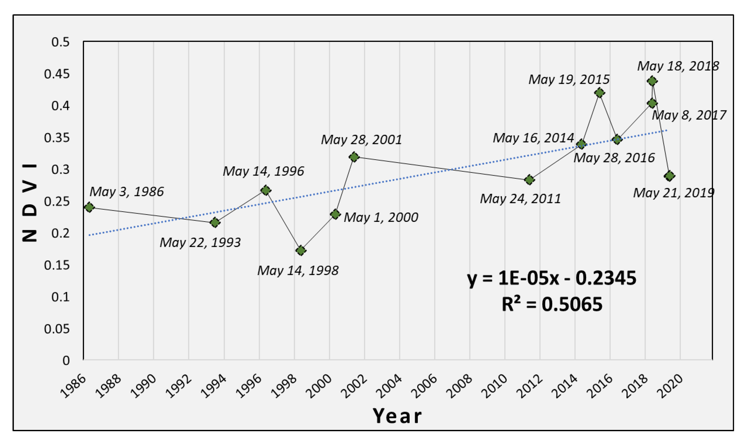
3.1. Results of the NDVI Analysis

After calculating the mean NDVI for each of the 80 UGSs across the 16 Landsat images, we combined all the NDVI values from all the parks by year to examine the yearly trend (Figure 5). The NDVI for all the parks increased slightly over time (p < 0.02), with significant variation from year to year. Similarly, we plotted the standard deviation of the 80 UGSs for each year (Figure 6). The standard deviation also increased slightly over time (p < 0.04).

Change over Time

To understand how each of the 80 UGSs changed over time, we compared the z-score of the 37 UGSs that had a positive z-score in 1986, meaning they were greener than average, against their z-score in 2019 (Figure 7). UGS de Santa Cruz (#67) had the highest z-score in 1986. This park was almost three standard deviations greener than the average park in 1986. During the 34-year period, the z-score of UGS de Santa Cruz declined to ~1.8, which is still much greener than the average UGS. Based on the fieldwork, we determined that the declining z-score of this UGS might be attributed to the reduction of canopy density, because this UGS is dominated by eucalyptus trees, with many of the trees going through senescence.
The golf club (#68) showed the second-highest z-score in 1986, which remained relatively stable when compared with its z-score in 2019. The relative consistency of this z-score is likely the result of heavy maintenance and irrigation. Three parks—Villa ATL (500,736 m2, #24), Cerro Amalucan (1,350,060 m2, #27), and state park Flor del Bosque (13,404,500 m2, #26)—also remained consistently green during the 34-year study period, despite minimal maintenance. This might be due to their vegetation and location; the vegetation cover of these three UGSs is mainly dominated by trees and other vegetation types that thrive in Puebla’s climate. In addition, they are relatively removed from the city core, which reduces human impact. However, as Puebla’s population increases, more human disruption is starting to occur. For example, in Flor del Bosque camping, hiking, and other recreational activities are now common. Similarly, in El Cerro Amalucan a large public swimming pool and dozens of studio rooms were inaugurated in 2020.
Of the three parks with the smallest positive z-scores in 1986, El Cri Cri (3009 m2, #69) experienced vegetation loss, Amanda (4273 m2, #10) remained relatively stable, and Strip-3 (5243 m2, #62) experienced vegetation loss as well. Of the three parks, Amanda has the most tree canopy and other types of vegetation cover, while the other two have some shrubs but also significant concrete surfaces. Of these 37 UGSs, La Luna park (#70) experienced the greatest loss in greenness, going from much greener than average in 1986 to much browner than average in 2019. La Luna is relatively new; before becoming a park, it was an empty lot covered with vegetation. When the lot became a park, its native vegetation was replaced with gravel, date palm trees, and shrubs. Similarly, the soccer field (#71) was an empty lot in 1986, which was converted to a soccer field by the Universidad Popular Autonoma del Estado de Puebla (UPAEP). During the conversion, grass was planted, and an irrigation system was installed. As a result, it experienced the strongest increase in greenness between 1986 and 2019. Los Enamorados park (#52) is covered mostly with Indian laurel trees, which have increased significantly in canopy area and density over the study period, and also shows a significant increase in greenness.
We also investigated the 43 UGSs that had a negative z-score in 1986 (Figure 8). There are only six UGSs–all parks–that converted from being browner than average in 1986, to becoming greener than average in 2019—Paseo San Francisco (#45), Ecopark Metropolitano of Puebla (#2), 2 de Octubre (#21), Jardin del Arte (#7), Jardines Paseo de San Francisco (58), and Las Ninjas (#40). Out of the six, Paseo San Francisco increased the most from −0.05 in 1986 to 1.9 in 2019. In addition, it is important to mention that three of these parks (Ecopark Metropolitano de Puebla, Paseo San Francisco, and Jardin del Arte) experienced major renovation during the study period. Vegetation cover was expanded as more trees were planted between 2011 and 2017. of the UGSs that were already browner than average in 1986, 20 experienced further loss in vegetation cover.

3.2. Hypothesis Testing

3.2.1. Hypothesis-1

Hypothesis-1: 
Indian Laurel Vegetation Effect.
To test whether UGS dominated by Indian laurel vegetation changed more significantly than UGS with other mixed vegetation types, we compared the slope of the regression line of the z-scores against years. The t-test results indicate that there is no significant difference (p = 0.30) between the rate of change of UGSs with mixed vegetation cover and the UGSs with Indian laurel tree vegetation cover. We also evaluated whether the UGSs with Indian laurel trees were greener on average. We found that there is a significant difference in the z-scores (p < 0.01) for the UGSs with mixed vegetation versus the UGSs with Indian laurel trees. It appears that even though the UGSs with Indian laurel trees did not reveal a significantly different rate of change, the UGSs with laurel trees are significantly greener overall than those with other vegetation types.

3.2.2. Hypothesis-2

Hypothesis-2: 
UGS Size Effect.
To understand whether the size of the UGSs impacts their greenness, we created a log-linear model linking the UGS size and the mean z-score over the 34-year period. The logistic regression model results (Figure 9) indicate that there is a significant relationship between the mean z-score and UGS size (p < 0.01). The majority of small UGSs have a negative mean z-score and the z-score increases for larger UGSs. About 31% of the variability in greenness is explained by the size of UGSs, with larger UGSs being significantly greener.
To understand if the size of the UGSs impacts how the greenness of the UGSs changed over time, we created a log-linear model linking UGS size and the rate of change of the z-score over the 34-year period. The logistic regression model results (Figure 10) indicate no significant relationship between UGS size and UGS change (p > 0.95). Thus, while larger UGSs are on average greener than smaller UGSs, we did not find that larger UGSs changed at a different rate than smaller UGSs.

3.2.3. Hypothesis-3

Hypothesis-3: 
UGS Maintenance Effect.
We also tested whether highly maintained and recently renovated UGSs showed a change in greenness significantly different from less maintained UGSs. We carried out a t-test to compare the change rate between 11 highly maintained or recently renovated UGSs (according to our field observations) and the other 69 UGSs. We did not find a significant difference (p < 0.54) between the two groups of UGSs. Figure 11 is an example of three selected parks that are highly maintained and their respective changes in NDVI, along with example images from Google Earth.

3.2.4. Paseo of San Francisco and El Centenario/Chapulco Lake

While we did not find a statistically significant difference between the rate of change for highly maintained parks and the level of maintenance, some of the highly maintained parks stood out. Among the 11 highly maintained or recently renovated parks, Paseo de San Francisco (#45) experienced the largest increase in greenness, while El Centenario/Chapulco Lake (#3) decreased the most in greenness (Figure 12). These parks followed a vastly different trajectory; as a result of renovations in Paseo de San Francisco, Indian laurel trees and other vegetation were planted; meanwhile, in El Centenario/Chapulco Lake more concrete was added, and the overgrown marshy waterbody was cleaned and aeration systems were installed, resulting in a drop in greenness.

3.3. Results from LST

In the following section, we present the results of the LST mean z-score and UGS size analysis, and LST change analysis. We also present the relationship of the LST mean z-score with the NDVI mean z-score formulated for 1 May 2000, 24 May 2011, and 21 May 2019.

3.3.1. LST Change and UGS Size

Figure 13 indicates a significant relationship (p < 0.01) between the size of the UGS and the average land surface temperature. Smaller UGSs were significantly warmer than larger UGSs (p < 0.01). Almost 50% of the variability in LST can be explained by the size of the UGS. Other biophysical and human-induced variables, such as location (distance to the city core), UGS greenness, vegetation cover, and maintenance, might explain the remaining variability in LST.

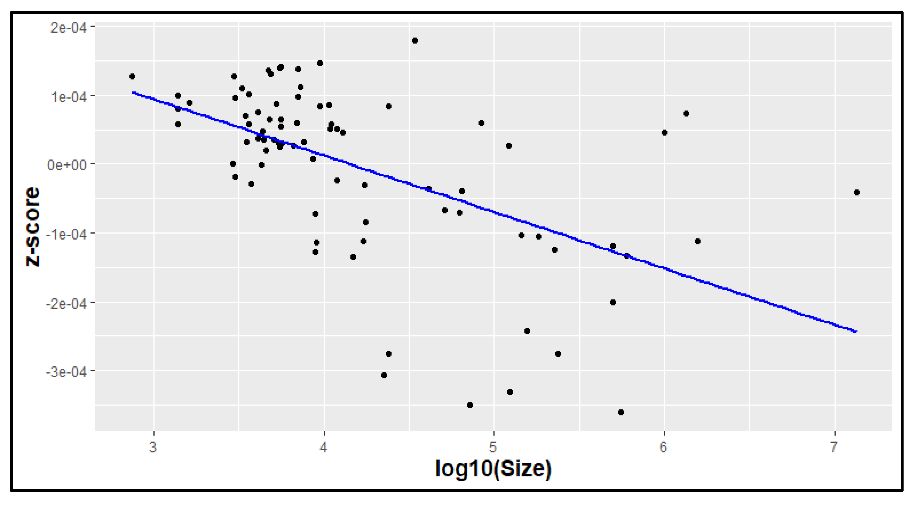
3.3.2. LST Z-Score Change and UGS Size

We also evaluated how the LST rate of change over the period of 20 years (2000–2019) varied with the size of the UGS (Figure 14). We found a significant relationship (p < 0.01) with larger UGSs revealing cooling over time (negative slopes), while smaller UGSs revealed slight warming or no change (rate of change was close to 0). Almost 30% of the change in the z-score can be explained by the size of UGS. Other biophysical and human-induced variables such as location (distance to the city core), UGS greenness, vegetation cover, and maintenance might explain the remaining changes in LST.

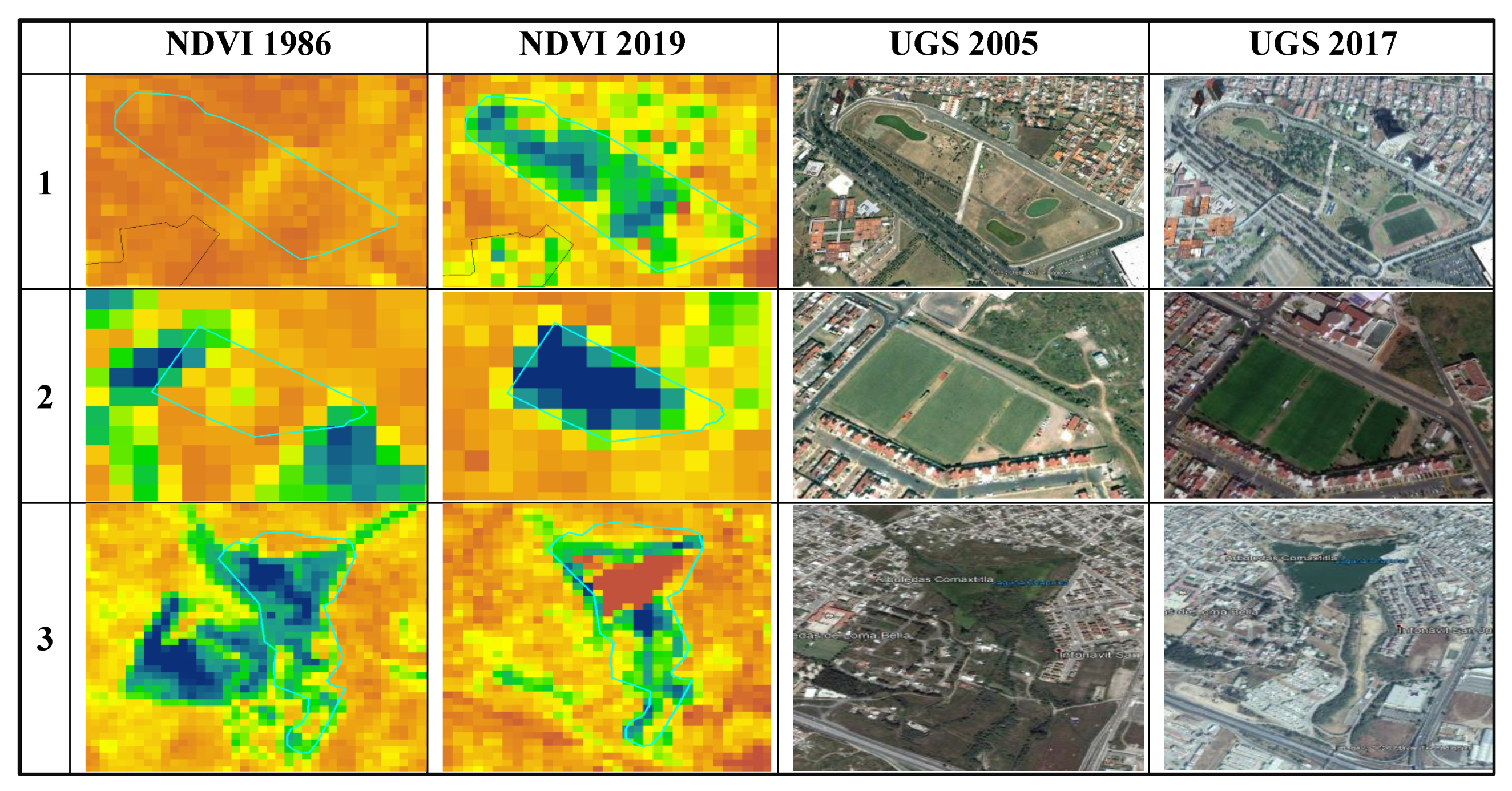
3.3.3. Detailed NDVI and LST Z-Score Analysis

To investigate the relationship between NDVI and LST, we selected observations from three different years—2000, 2011, and 2019—to see whether changes occurred over time. Figure 15 visualizes the data from 1 May 2000 and reveals a negative relationship between the NDVI and LST values (p < 0.01). About 16.5% of the variability in the LST z-score of the UGS can be explained by the z-score of the NDVI. The weak relationship shows that in the year 2000, greener parks were slightly cooler than browner parks and that those differences depended on vegetation cover types. For example, parks covered with trees (cooler-browner quadrant) were cooler than parks with grass cover (warmer-browner quadrant) of similar size.
UGSs in the upper left quadrant (warmer-browner quadrant) and the lower right quadrant (cooler-greener quadrant) generally show lower temperatures for areas with high vegetation cover. UGSs in the lower left quadrant (cooler-browner quadrant) show a different trend. At least one of those UGSs (Lake of Saint Baltazar) has a large waterbody, which could explain its relative coolness. UGSs in the upper right quadrant (warmer-greener), such as La Constancia/Paseo de Los Gigantes (#39), El Ameyal (#20), and Neighborhood Case-1 (#60) and Case-2 (#5), are relatively warm compared to their above-average greenness.
The relationship between NDVI and LST appears to strengthen over time, with R2adj values increasing from 0.17 in 2000, to 0.37 in 2011 (Figure 16), and 0.42 in 2019 (Figure 17). This might be a result of the UGS digitization based on modern high-resolution satellite imagery.
Most UGSs in 2011 match the general theory that greener areas are cooler. Exceptions are parks with large waterbodies (e.g., Lake of Saint Baltazar (#4)) where a browner than average UGS resulted in a cooler than average observation. This is not surprising considering that water is generally cooler than other land cover classes, and the NDVI values for water are generally low. Other UGSs, such as the soccer field, also divert from the general trend. While the soccer field is relatively green, it provides no shading resulting in slightly warmer than average temperatures.
Figure 17 shows El Centenario/Chapulco Lake and Lake of Saint Baltazar in close proximity in the cooler-browner quadrant. Both UGSs have extensive waterbodies. Not all UGSs were fully established in 2000. El Centenario/Chapulco Lake is a relatively new park that used to be an overgrown marshy area. The establishment of this park resulted in a reduction of the vegetation cover in the park’s area. Marshy water was cleaned, which resulted in lower LST (Figure 17). Overall, we found that highly maintained UGSs generally increased in greenness (Paseo de San Francisco, Jardin del Arte, Ecopark Metropolitano de Puebla (includes a Baroque Museum), and Ecopark Mexican Revolution).
The soccer field (#71) and El Ameyal (#20) also appear as outliers, with high NDVI values and high land surface temperatures. These areas are covered with grass, which does not produce shade, resulting in higher LST as well. The opposite trend is observed with UGSs in the cooler-greener quadrant (Paseo de San Francisco (#45), Paseo Bravo (#46), Benito Juarez (#19), and University (#75). Those parks are mostly covered with Indian laurel trees, and over the study period the trees increased in height and in vegetation density, resulting in a decrease in LST. These results lead us to conclude that shade and canopy density are vital variables for the remediation of UHI. Furthermore, an interesting relationship is observed for the golf club, which consistently has high NDVI and low LST. While the golf club is mostly covered with grass, it also has more than 40% tree cover. This private golf club is also highly irrigated to keep the grass pristine, leading us to conclude that soil moisture and potential evaporation from irrigation causes lower LST.

4. Discussion

In this study, we examined the NDVI from 80 urban green spaces (UGSs) over a 34-year period and its relationship with UGS size and Indian laurel tree cover. We also analyzed the trajectories of LST during a 20-year period in relation to UGS size. Finally, we investigated the relationship between the NDVI z-score and the LST z-score during the 2000–2019 period. We visually inspected 73 of the 80 UGSs to better understand their land cover types and other characteristics. Our study reveals that each UGS displayed different drivers of change in NDVI, including biophysical processes, human-induced changes, and local climate impacts. We found significant variability in the results, with some UGSs revealing significant greening while other UGSs revealed greenness declines. Similar variability was found for the land surface temperature (LST) trajectories, although in general, large UGSs were cooler compared to small ones. We also found that shaded UGSs and those with large waterbodies were generally cooler.
The results of this study are consistent with a previous study that reported contrasting NDVI changes by comparing specific neighborhoods in Chicago in 1998 and 2010 [43]. We also found contrasting NDVI changes, and we observed that the standard deviation widened over time.
We were able to examine vegetation cover differences at a local scale, and we found that UGSs with Indian laurel were significantly greener than UGSs with mixed vegetation cover, although the change rate was not different for UGSs with Indian laurel. We also found that the type of vegetation cover mattered for the LST relationship. UGSs with grass covers, such as the soccer field (in 2019), Neighborhood Case-1, and Neighborhood Case-2 (2010), were relatively warm compared to other UGSs because these grassy UGSs lacked shade. Other studies also linked lower surface temperatures with increased shading, high evapotranspiration [70], vegetation types, canopy density [71], and tree cover [72]. Soil temperature differences beneath trees and shrubs are lower compared to herbaceous and grass cover in the summer months [73]. Similarly, the surface temperature of grass is generally lower than asphalt or concrete [74].
In accordance with other studies, we found that UGSs with large waterbodies (>128,889 m2) are generally cooler [75,76]. El Centenario/Chapulco Lake (227,050 m2) and Lake Saint Baltazar (143,629 m2) had lower LST compared to similar size UGSs without waterbodies. Waterbodies and dense urban green infrastructure were also found to lower LST in two Indian cities [77]. Water has a higher heat capacity than vegetation, and most of the solar radiation is absorbed [78,79] and subsequently released at a later time. As a result, while water might be cooler in daytime images, it would be warmer during the night. We demonstrated that large UGSs are generally greener compared to smaller UGSs, which is consistent with what other studies have concluded. By examining 39 parks, Lin et al. [25] concluded that larger parks provide higher NDVI values, resulting in a cooling effect [25]. Other studies also conclude that vegetation, water, and impervious surface cover determine LST [80,81,82].
Multiple studies have investigated the relationship between urbanization and UHI. One study found a positive relationship between the urban area and LST across 419 global big cities [83]. This study also found that the size of the urban area explains up to 87% of the variance in UHI. As urban expansion continues worldwide it is important to preserve and build a network of UGSs to reduce surface and air temperatures. Urban green infrastructure can reduce the energy demand and consumption for cooling [84,85] and alleviate the UHI impact [86].
Previous studies that have examined the relationship between UGSs and UHI on a city scale have predominantly used data for one year, a summer season, or in some cases a single date [26,87,88], except for Mackey et al. [43], who examined UGSs in Chicago for a 12-year period (1998–2010). Similarly, many studies treat UGSs as static [89,90,91,92]. Cognizant of this limitation, our study used more than 30 years of data and treated the UGSs as transient entities. Using z-scores to investigate changes within UGSs and across UGSs, allowed us to understand the variability in greenness. Field observations for 73 of the 80 UGSs allowed us to learn differences in land cover, vegetation types, vegetation changes (as is the case with Jacaranda flowering), maintenance, and infrastructure characteristics for each UGS. We highlight Park Federico Escobedo (#32), which was mostly covered by Jacaranda trees (Figure 6) and was found “greener” and warmer than average on 21 May 2019 (Figure 17). The month of May is the blooming season of the Jacaranda trees, resulting in higher NDVI but also higher LST because the flowers are mainly in the upper layer of the canopy, resulting in limited shade and warmer-than-average temperatures. Canopy layers in vegetation result in strong shading and robust shade results in lower LST.
While we visited the UGSs, we often talked to park users to learn about the story of the park and gather the information that was not available through online databases. In these discussions, we learned that the renovation of Park El Centenario/Chapulco Lake, counter-intuitively, resulted in a reduction of vegetation cover as impervious surfaces were added. During the renovation, the lake was also cleaned up, and several aeration systems were installed to keep the water circulating. As a result, we found that the LST values, which are typically already lower for water bodies, dropped significantly. However, not all renovations resulted in a decrease in LST. For example, in Los Fuertes (#29, which displays monuments and statues of the battle of Cinco de Mayo, a museum, and coffee shops), and in La Constancia/Paseo de Los Gigantes (#39, which is a model park showcasing iconic buildings from around world, a museum, and a coffee shop), aesthetic and cultural displays were prioritized over environmental benefits. Field observations also improved our understanding of vegetation cover differences. We learned that Eucalyptus trees dominate the Cerro Amalucan park (#27, Figure 6). Eucalyptus has a single main stem and is a fast-growing tree, ranging from 10 m to 60 m in height. However, with low canopy density and with long, slender, downward pointing leaves (7–10 cm), these trees generate limited shade. Cerro Amalucan park is one of the largest UGSs in our study. Los Fuertes park also has Eucalyptus trees and other vegetation and about 45% of the park is covered with impervious surfaces that include roads, parking lots, museums, and a statue with personages commemorating the Cinco de Mayo, Battle of Puebla. [29]

5. Conclusions

As urban populations continue to increase, urbanization encroachment in the vegetated landscapes is more likely to continue, resulting in the increase of UHI. For the cities located in the lower latitudes, the UHI increase is more acute than for cities in higher latitudes [47], because they receive more solar radiation year-round, which in the summer months is exacerbated further. Monitoring the health of UGSs and their relationship with LST is important to better understand how cities can implement and maintain urban green infrastructure. Our study intends to bridge the geographic asymmetries in the cities studied for UHI [29]. Most studies of UHI and urban green spaces predominantly look at parks that are concentrated in just a handful of countries and their respective cities. While some UHI studies have been conducted in Puebla (Mexico), to our knowledge, this is the first study where optical and thermal remotely sensed data are used to examine greenness and LST in urban green spaces. This study intends to reduce the gaps in scholarship identified in the literature review of UHI [29]. We found that small UGSs are not as effective at reducing UHI compared to larger UGSs. Similarly, the cooling intensity directly depends on land cover characteristics, because large UGSs with portions of impervious surfaces or bare land might not be as effective in temperature reduction as UGSs with more vegetated areas. Equivalently sized UGSs with similar NDVI results presented different LST values, and this difference was largely dependent on shadow effects. Unfortunately, our dataset does not have enough statistical power to quantitatively distinguish between parks with shadow effects and those without. Nevertheless, UGSs mostly covered with trees had lower LST than UGSs primarily covered with grasses. Likewise, UGSs with large water bodies were more effective at reducing daytime LST, although we did not investigate nighttime data.
UGSs vegetated with Indian laurel trees were greener than UGSs with mixed cover and were more stable. Moreover, Indian laurel trees have dense canopy layers with an oblate shape, which provide more shade resulting in more cooling compared to Eucalyptus, grass cover, etc. While newly planted Indian laurel trees require intense watering to grow their roots, once the trees are established, watering can be eliminated because they are drought-resistant compared to grass, flowers, and other ornamental shrubs. Planting Indian laurel trees in UGSs in Puebla can be a good xeriscaping practice and may yield the most ecosystem services compared to other succulent plants, grasses, or other ornamental shrubs.

Author Contributions

Conceptualization, F.G.-M. and K.M.d.B.; methodology, F.G.-M.; software, K.M.d.B.; field validation, F.G.-M.; formal analysis, F.G.-M.; writing—original draft preparation, F.G.-M.; writing—review and editing, F.G.-M., K.M.d.B., J.K., and J.W.; visualization, F.G.-M.; supervision, K.M.d.B.; All authors have read and agreed to the published version of the manuscript.

Funding

This research received not external funding.

Data Availability Statement

The park photographs of this study are available at: https://arcg.is/1nqnnL.

Acknowledgments

Authors would like to acknowledge work by Paul de Beurs to enable to development of the land surface temperature data. In Puebla, we would like to thank Estefania Martinez Tavera (UPAEP) for providing contact of INEGI, and IMPLAN personnel, Hugo Vasquez Cabrera (INEGI), Norman Campos Velasquez and Diana Hernandez Navarro (IMPLAN), Claudia Magallanes Blanco (Ibero-Puebla), Leandro Rodriguez Medina (UDLAP), and Oscar Tamayo Vivas and family for driving around Puebla. We would like to thank Laurel Smith for her suggestions on the writing of the beginnings of this manuscript. We thank Braden Owsley for his assistance with English language editing. We would also like to thank three anonymous reviewers for their valuable and insightful comments on an earlier version of this manuscript.

Conflicts of Interest

The authors declare no conflict of interest.

References

  1. UN DESA. 68% of the World Population Projected to Live in Urban Areas by 2050, Says UN|UN DESA|United Nations Department of Economic and Social Affairs. Available online: https://www.un.org/development/desa/en/news/population/2018-revision-of-world-urbanization-prospects.html (accessed on 27 December 2020).
  2. McKinney, M.L. Urbanization, Biodiversity, and Conservation. BioScience 2002, 52, 883. [Google Scholar] [CrossRef]
  3. Shuster, W.D.; Bonta, J.; Thurston, H.; Warnemuende, E.; Smith, D.R. Impacts of Impervious Surface on Watershed Hydrology: A Review. Urban Water 2005, 2, 263–275. [Google Scholar] [CrossRef]
  4. Hammond, M.J.; Chen, A.S.; Djordjević, S.; Butler, D.; Mark, O. Urban Flood Impact Assessment: A State-of-the-Art Review. Urban Water 2015, 12, 14–29. [Google Scholar] [CrossRef] [Green Version]
  5. Santamouris, M.; Cartalis, C.; Synnefa, A.; Kolokotsa, D. On the Impact of Urban Heat Island and Global Warming on the Power Demand and Electricity Consumption of Buildings—A Review. Energy Build. 2015, 98, 119–124. [Google Scholar] [CrossRef]
  6. Santamouris, M.; Kolokotsa, D. On the Impact of Urban Overheating and Extreme Climatic Conditions on Housing, Energy, Comfort and Environmental Quality of Vulnerable Population in Europe. Energy Build. 2015, 98, 125–133. [Google Scholar] [CrossRef]
  7. Polydoros, A.; Cartalis, C. Use of Earth Observation Based Indices for the Monitoring of Built-up Area Features and Dynamics in Support of Urban Energy Studies. Energy Build. 2015, 98, 92–99. [Google Scholar] [CrossRef]
  8. Zhao, J.; Wang, J.; Jin, Y.; Fan, L.; Xu, C.; Liang, D.; Huang, L. Land Cover Based Landscape Pattern Dynamics of Anhui Province Using GlobCover and MCD12Q1 Global Land Cover Products. Sustainability 2018, 10, 1285. [Google Scholar] [CrossRef] [Green Version]
  9. Liu, Y.; Peng, J.; Wang, Y. Efficiency of Landscape Metrics Characterizing Urban Land Surface Temperature. Landsc. Urban Plan. 2018, 180, 36–53. [Google Scholar] [CrossRef]
  10. Maimaitiyiming, M.; Ghulam, A.; Tiyip, T.; Pla, F.; Latorre-Carmona, P.; Halik, Ü.; Sawut, M.; Caetano, M. Effects of Green Space Spatial Pattern on Land Surface Temperature: Implications for Sustainable Urban Planning and Climate Change Adaptation. ISPRS J. Photogramm. Remote Sens. 2014, 89, 59–66. [Google Scholar] [CrossRef] [Green Version]
  11. Voogt, J.A.; Oke, T.R. Thermal Remote Sensing of Urban Climates. Remote Sens. Environ. 2003, 86, 370–384. [Google Scholar] [CrossRef]
  12. Yagüe, C.; Zurita, E.; Martinez, A. Statistical Analysis of the Madrid Urban Heat Island. Atmos. Environ. Part B Urban Atmos. 1991, 25, 327–332. [Google Scholar] [CrossRef]
  13. Rosenzweig, C.; Solecki, W.D.; Parshall, L.; Chopping, M.; Pope, G.; Goldberg, R. Characterizing the Urban Heat Island in Current and Future Climates in New Jersey. Environ. Hazards 2005, 6, 51–62. [Google Scholar] [CrossRef]
  14. Vidrih, B.; Medved, S. Multiparametric Model of Urban Park Cooling Island. Urban For. Urban Green. 2013, 12, 220–229. [Google Scholar] [CrossRef]
  15. Zhang, Y.; Zhan, Y.; Yu, T.; Ren, X. Urban Green Effects on Land Surface Temperature Caused by Surface Characteristics: A Case Study of Summer Beijing Metropolitan Region. Infrared Phys. Technol. 2017, 86, 35–43. [Google Scholar] [CrossRef]
  16. Li, H.; Zhou, Y.; Li, X.; Meng, L.; Wang, X.; Wu, S.; Sodoudi, S. A New Method to Quantify Surface Urban Heat Island Intensity. Sci. Total Environ. 2018, 624, 262–272. [Google Scholar] [CrossRef] [PubMed]
  17. Mills, G. and Luke Howard. The Climate of London. Weather 2008, 63, 153–157. [Google Scholar] [CrossRef]
  18. Carlson, T.N.; Augustine, J.A.; Boland, F.E. Potential Application of Satellite Temperature Measurements in the Analysis of Land Use over Urban Areas. Bull. Am. Meteorol. Soc. 1977, 58, 1301–1303. Available online: https://www.jstor.org/stable/26218022 (accessed on 21 April 2020).
  19. Oke, T.R. The Energetic Basis of the Urban Heat Island. Q. J. R. Meteorol. Soc. 1982, 108, 1–24. [Google Scholar] [CrossRef]
  20. Ren, Z.; He, X.; Zheng, H.; Zhang, D.; Yu, X.; Shen, G.; Guo, R. Estimation of the Relationship between Urban Park Characteristics and Park Cool Island Intensity by Remote Sensing Data and Field Measurement. Forests 2013, 4, 868–886. [Google Scholar] [CrossRef] [Green Version]
  21. Yuan, F.; Bauer, M.E. Comparison of Impervious Surface Area and Normalized Difference Vegetation Index as Indicators of Surface Urban Heat Island Effects in Landsat Imagery. Remote Sens. Environ. 2007, 106, 375–386. [Google Scholar] [CrossRef]
  22. Hamada, S.; Ohta, T. Seasonal Variations in the Cooling Effect of Urban Green Areas on Surrounding Urban Areas. Urban For. Urban Green. 2010, 9, 15–24. [Google Scholar] [CrossRef]
  23. Hamilton, S.K.; Hussain, M.Z.; Lowrie, C.; Basso, B.; Robertson, G.P. Evapotranspiration Is Resilient in the Face of Land Cover and Climate Change in a Humid Temperate Catchment. Hydrol. Process. 2018, 32, 655–663. [Google Scholar] [CrossRef] [Green Version]
  24. Trlica, A.; Hutyra, L.R.; Schaaf, C.L.; Erb, A.; Wang, J.A. Albedo, Land Cover, and Daytime Surface Temperature Variation Across an Urbanized Landscape: Albedo of urban landscape. Earth Future 2017, 5, 1084–1101. [Google Scholar] [CrossRef] [Green Version]
  25. Lin, W.; Yu, T.; Chang, X.; Wu, W.; Zhang, Y. Calculating Cooling Extents of Green Parks Using Remote Sensing: Method and Test. Landsc. Urban Plan. 2015, 134, 66–75. [Google Scholar] [CrossRef]
  26. Chang, C.-R.; Li, M.-H. Effects of Urban Parks on the Local Urban Thermal Environment. Urban For. Urban Green. 2014, 13, 672–681. [Google Scholar] [CrossRef]
  27. Zhang, S.; Zhou, W. Recreational Visits to Urban Parks and Factors Affecting Park Visits: Evidence from Geotagged Social Media Data. Landsc. Urban Plan. 2018, 180, 27–35. [Google Scholar] [CrossRef]
  28. von Döhren, P.; Haase, D. Ecosystem Disservices Research: A Review of the State of the Art with a Focus on Cities. Ecol. Indic. 2015, 52, 490–497. [Google Scholar] [CrossRef]
  29. Zhou, D.; Xiao, J.; Bonafoni, S.; Berger, C.; Deilami, K.; Zhou, Y.; Frolking, S.; Yao, R.; Qiao, Z.; Sobrino, J. Satellite Remote Sensing of Surface Urban Heat Islands: Progress, Challenges, and Perspectives. Remote Sens. 2018, 11, 48. [Google Scholar] [CrossRef] [Green Version]
  30. Dobbs, C.; Escobedo, F.J.; Clerici, N.; de la Barrera, F.; Eleuterio, A.A.; MacGregor-Fors, I.; Reyes-Paecke, S.; Vásquez, A.; Zea Camaño, J.D.; Hernández, H.J. Urban Ecosystem Services in Latin America: Mismatch between Global Concepts and Regional Realities? Urban Ecosyst. 2019, 22, 173–187. [Google Scholar] [CrossRef]
  31. Arocena, R.; Senker, P. Technology, Inequality, and Underdevelopment: The Case of Latin America. Sci. Technol. Hum. Values 2003, 28, 15–33. [Google Scholar] [CrossRef]
  32. Alcorta, L.; Peres, W. Innovation Systems and Technological Specialization in Latin America and the Caribbean. Res. Policy 1998, 26, 857–881. [Google Scholar] [CrossRef] [Green Version]
  33. Eakin, H.; Lemos, M.C. Adaptation and the State: Latin America and the Challenge of Capacity-Building under Globalization. Glob. Environ. Chang. 2006, 16, 7–18. [Google Scholar] [CrossRef]
  34. Devlin, R.; Moguillansky, G. What’s New in the New Industrial Policy in Latin America? In The Industrial Policy Revolution I: The Role of Government beyond Ideology; Stiglitz, J.E., Lin, J.Y., Eds.; Palgrave Macmillan: London, UK, 2013; pp. 276–317. ISBN 978-1-137-33517-3. [Google Scholar]
  35. INEGI México En Cifras. Available online: https://www.inegi.org.mx/app/areasgeograficas/?ag=21 (accessed on 3 December 2020).
  36. Jauregui, E. Mexico City’s Urban Heat Island Revisited. Erdkunde 1993, 47, 185–195. [Google Scholar] [CrossRef]
  37. Ballinas, M.; Barradas, V.L. The Urban Tree as a Tool to Mitigate the Urban Heat Island in Mexico City: A Simple Phenomenological Model. J. Environ. Qual. 2016, 45, 157–166. [Google Scholar] [CrossRef]
  38. Cui, Y.Y.; de Foy, B. Seasonal Variations of the Urban Heat Island at the Surface and the Near-Surface and Reductions Due to Urban Vegetation in Mexico City. J. Appl. Meteorol. Climatol. 2012, 51, 855–868. [Google Scholar] [CrossRef]
  39. Rivera, E.; Antonio-Némiga, X.; Origel-Gutiérrez, G.; Sarricolea, P.; Adame-Martínez, S. Spatiotemporal Analysis of the Atmospheric and Surface Urban Heat Islands of the Metropolitan Area of Toluca, Mexico. Environ. Earth Sci. 2017, 76, 225. [Google Scholar] [CrossRef]
  40. Jauregui, E.; Godinez, L.; Cruz, F. Aspects of Heat-Island Development in Guadalajara, Mexico. Atmos. Environ. Part B Urban Atmos. 1992, 26, 391–396. [Google Scholar] [CrossRef]
  41. Villanueva-Solis, J. Urban Heat Island Mitigation and Urban Planning: The Case of the Mexicali, B.C. Mexico. Am. J. Clim. Chang. 2017, 6, 22–39. [Google Scholar] [CrossRef] [Green Version]
  42. Abarca, K.M.N.; De Lara, C.F.; Hernandez, A.S.; Leon, M.T. Evaluation of urban heat island for Puebla City, Mexico. Sustain. Dev. Plan. 2018, 867–879. [Google Scholar] [CrossRef] [Green Version]
  43. Mackey, C.W.; Lee, X.; Smith, R.B. Remotely Sensing the Cooling Effects of City Scale Efforts to Reduce Urban Heat Island. Build. Environ. 2012, 49, 348–358. [Google Scholar] [CrossRef]
  44. Glenn, E.; Huete, A.; Nagler, P.; Nelson, S. Relationship Between Remotely-Sensed Vegetation Indices, Canopy Attributes and Plant Physiological Processes: What Vegetation Indices Can and Cannot Tell Us About the Landscape. Sensors 2008, 8, 2136–2160. [Google Scholar] [CrossRef] [Green Version]
  45. Zhu, Z.; Zhou, Y.; Seto, K.C.; Stokes, E.C.; Deng, C.; Pickett, S.T.A.; Taubenböck, H. Understanding an Urbanizing Planet: Strategic Directions for Remote Sensing. Remote Sens. Environ. 2019, 228, 164–182. [Google Scholar] [CrossRef]
  46. Duan, J.; Wang, Y.; Fan, C.; Xia, B.; de Groot, R. Perception of Urban Environmental Risks and the Effects of Urban Green Infrastructures (UGIs) on Human Well-Being in Four Public Green Spaces of Guangzhou, China. Environ. Manag. 2018, 62, 500–517. [Google Scholar] [CrossRef] [PubMed]
  47. Gibson, S.C. “Let’s Go to the Park.” An Investigation of Older Adults in Australia and Their Motivations for Park Visitation. Landsc. Urban Plan. 2018, 180, 234–246. [Google Scholar] [CrossRef]
  48. Kondo, M.; Fluehr, J.; McKeon, T.; Branas, C. Urban Green Space and Its Impact on Human Health. Int. J. Environ. Res. Public Health 2018, 15, 445. [Google Scholar] [CrossRef] [Green Version]
  49. Kothencz, G.; Kolcsár, R.; Cabrera-Barona, P.; Szilassi, P. Urban Green Space Perception and Its Contribution to Well-Being. Int. J. Environ. Res. Public Health 2017, 14, 766. [Google Scholar] [CrossRef] [Green Version]
  50. Choumert, J.; Salanié, J. Provision of Urban Green Spaces: Some Insights from Economics. Landsc. Res. 2008, 33, 331–345. [Google Scholar] [CrossRef]
  51. AtmosCor Atmospheric Correction Parameter Calculator. Available online: https://atmcorr.gsfc.nasa.gov/ (accessed on 3 December 2020).
  52. IMPLAN Inicio. Available online: http://implan.pueblacapital.gob.mx/ (accessed on 3 December 2020).
  53. Elvidge, C.D.; Chen, Z. Comparison of Broad-Band and Narrow-Band Red and near-Infrared Vegetation Indices. Remote Sens. Environ. 1995, 54, 38–48. [Google Scholar] [CrossRef]
  54. Tucker, C.J. Red and Photographic Infrared Linear Combinations for Monitoring Vegetation. Remote Sens. Environ. 1979, 8, 127–150. [Google Scholar] [CrossRef] [Green Version]
  55. Baret, F.; Guyot, G. Potentials and Limits of Vegetation Indices for LAI and APAR Assessment. Remote Sens. Environ. 1991, 35, 161–173. [Google Scholar] [CrossRef]
  56. Huete, A.R.; Jackson, R.D.; Post, D.F. Spectral Response of a Plant Canopy with Different Soil Backgrounds. Remote Sens. Environ. 1985, 17, 37–53. [Google Scholar] [CrossRef]
  57. Qin, Z.; Karnieli, A.; Berliner, P. A Mono-Window Algorithm for Retrieving Land Surface Temperature from Landsat TM Data and Its Application to the Israel-Egypt Border Region. Int. J. Remote Sens. 2001, 22, 3719–3746. [Google Scholar] [CrossRef]
  58. Jiménez-Muñoz, J.C.; Sobrino, J.A. A Generalized Single-channel Method for Retrieving Land Surface Temperature from Remote Sensing Data. J. Geophys. Res. 2003, 108. [Google Scholar] [CrossRef] [Green Version]
  59. Halthore, R.N. Intercomparison of Shortwave Radiative Transfer Codes and Measurements. J. Geophys. Res. 2005, 110, D11206. [Google Scholar] [CrossRef] [Green Version]
  60. Li, Z.-L.; Wu, H.; Wang, N.; Qiu, S.; Sobrino, J.A.; Wan, Z.; Tang, B.-H.; Yan, G. Land Surface Emissivity Retrieval from Satellite Data. Int. J. Remote Sens. 2013, 34, 3084–3127. [Google Scholar] [CrossRef]
  61. Windahl, E.; de Beurs, K.M. An Intercomparison of Landsat Land Surface Temperature Retrieval Methods under Variable Atmospheric Conditions Using in Situ Skin Temperature. Int. J. Appl. Earth Obs. Geoinf. 2016, 51, 11–27. [Google Scholar] [CrossRef] [Green Version]
  62. Tang, H.; Li, Z.-L. Quantitative Remote Sensing in Thermal Infrared; Springer Remote Sensing/Photogrammetry; Springer: Berlin/Heidelberg, Germany, 2014; ISBN 978-3-642-42026-9. [Google Scholar]
  63. Sobrino, J.A.; Jiménez-Muñoz, J.C.; Paolini, L. Land Surface Temperature Retrieval from LANDSAT TM 5. Remote Sens. Environ. 2004, 90, 434–440. [Google Scholar] [CrossRef]
  64. Peres, L.F.; DaCamara, C.C. Emissivity Maps to Retrieve Land-Surface Temperature from MSG/SEVIRI. IEEE Trans. Geosci. Remote Sens. 2005, 43, 1834–1844. [Google Scholar] [CrossRef]
  65. Wang, X.; OuYang, X.; Tang, B.; Li, Z.-L.; Zhang, R. A New Method for Temperature/Emissivity Separation from Hyperspectral Thermal Infrared Data. In Proceedings of the IGARSS 2008—2008 IEEE International Geoscience and Remote Sensing Symposium, Boston, MA, USA, 7–11 July 2008; pp. III-286–III-289. [Google Scholar]
  66. Li, Z.; Petitcolin, F.; Zhang, R. A Physically Based Algorithm for Land Surface Emissivity Retrieval from Combined Mid-Infrared and Thermal Infrared Data. Sci. China Ser. E Technol. Sci. 2000, 43, 23–33. [Google Scholar] [CrossRef]
  67. Van de Griend, A.A.; Owe, M.E. On the Relationship between Thermal Emissivity and the Normalized Difference Vegetation Index for Natural Surfaces. Int. J. Remote Sens. 1993, 14, 1119–1131. [Google Scholar] [CrossRef]
  68. Hulley, G.C.; Hook, S.J. The North American ASTER Land Surface Emissivity Database (NAALSED) Version 2.0. Remote Sens. Environ. 2009, 113, 1967–1975. [Google Scholar] [CrossRef]
  69. Chander, G.; Markham, B.L.; Helder, D.L. Summary of Current Radiometric Calibration Coefficients for Landsat MSS, TM, ETM+, and EO-1 ALI Sensors. Remote Sens. Environ. 2009, 113, 893–903. [Google Scholar] [CrossRef]
  70. Alexander, C. Normalised Difference Spectral Indices and Urban Land Cover as Indicators of Land Surface Temperature (LST). Int. J. Appl. Earth Obs. Geoinf. 2020, 86, 102013. [Google Scholar] [CrossRef]
  71. Feyisa, G.L.; Dons, K.; Meilby, H. Efficiency of Parks in Mitigating Urban Heat Island Effect: An Example from Addis Ababa. Landsc. Urban Plan. 2014, 123, 87–95. [Google Scholar] [CrossRef]
  72. Dugord, P.-A.; Lauf, S.; Schuster, C.; Kleinschmit, B. Land Use Patterns, Temperature Distribution, and Potential Heat Stress Risk—The Case Study Berlin, Germany. Comput. Environ. Urban Syst. 2014, 48, 86–98. [Google Scholar] [CrossRef]
  73. Edmondson, J.L.; Stott, I.; Davies, Z.G.; Gaston, K.J.; Leake, J.R. Soil Surface Temperatures Reveal Moderation of the Urban Heat Island Effect by Trees and Shrubs. Sci. Rep. 2016, 6, 33708. [Google Scholar] [CrossRef] [PubMed] [Green Version]
  74. Ziter, C.D.; Pedersen, E.J.; Kucharik, C.J.; Turner, M.G. Scale-Dependent Interactions between Tree Canopy Cover and Impervious Surfaces Reduce Daytime Urban Heat during Summer. Proc. Natl. Acad. Sci. USA 2019, 116, 7575. [Google Scholar] [CrossRef] [PubMed] [Green Version]
  75. Kong, F.; Yin, H.; Wang, C.; Cavan, G.; James, P. A Satellite Image-Based Analysis of Factors Contributing to the Green-Space Cool Island Intensity on a City Scale. Urban For. Urban Green. 2014, 13, 846–853. [Google Scholar] [CrossRef] [Green Version]
  76. Chen, X.; Su, Y.; Li, D.; Huang, G.; Chen, W.; Chen, S. Study on the Cooling Effects of Urban Parks on Surrounding Environments Using Landsat TM Data: A Case Study in Guangzhou, Southern China. Int. J. Remote Sens. 2012, 33, 5889–5914. [Google Scholar] [CrossRef]
  77. Ramaiah, M.; Avtar, R.; Rahman, M.M. Land Cover Influences on LST in Two Proposed Smart Cities of India: Comparative Analysis Using Spectral Indices. Land 2020, 9, 292. [Google Scholar] [CrossRef]
  78. Gunawardena, K.R.; Wells, M.J.; Kershaw, T. Utilising Green and Bluespace to Mitigate Urban Heat Island Intensity. Sci. Total Environ. 2017, 584–585, 1040–1055. [Google Scholar] [CrossRef]
  79. Cheng, X.; Wei, B.; Chen, G.; Li, J.; Song, C. Influence of Park Size and Its Surrounding Urban Landscape Patterns on the Park Cooling Effect. J. Urban Plan. Dev. 2015, 141, A4014002. [Google Scholar] [CrossRef]
  80. Cheng, L.; Guan, D.; Zhou, L.; Zhao, Z.; Zhou, J. Urban Cooling Island Effect of Main River on a Landscape Scale in Chongqing, China. Sustain. Cities Soc. 2019, 47, 101501. [Google Scholar] [CrossRef]
  81. Ezimand, K.; Kakroodi, A.A.; Kiavarz, M. The Development of Spectral Indices for Detecting Built-up Land Areas and Their Relationship with Land-Surface Temperature. Int. J. Remote Sens. 2018, 39, 8428–8449. [Google Scholar] [CrossRef]
  82. Zhang, X.; Zhong, T.; Wang, K.; Cheng, Z. Scaling of Impervious Surface Area and Vegetation as Indicators to Urban Land Surface Temperature Using Satellite Data. Int. J. Remote Sens. 2009, 30, 841–859. [Google Scholar] [CrossRef]
  83. Peng, S.; Piao, S.; Ciais, P.; Friedlingstein, P.; Ottle, C. Surface Urban Heat Island Across 419 Global Big Cities. Environ. Sci. Technol. 2012, 46, 696–703. [Google Scholar] [CrossRef]
  84. Pandit, R.; Laband, D.N. Energy Savings from Tree Shade. Ecol. Econ. 2010, 69, 1324–1329. [Google Scholar] [CrossRef]
  85. Akbari, H.; Kolokotsa, D. Three Decades of Urban Heat Islands and Mitigation Technologies Research. Energy Build. 2016, 133, 834–842. [Google Scholar] [CrossRef]
  86. Chen, J.; Jin, S.; Du, P. Roles of Horizontal and Vertical Tree Canopy Structure in Mitigating Daytime and Nighttime Urban Heat Island Effects. Int. J. Appl. Earth Obs. Geoinf. 2020, 89, 102060. [Google Scholar] [CrossRef]
  87. Bokaie, M.; Zarkesh, M.K.; Arasteh, P.D.; Hosseini, A. Assessment of Urban Heat Island Based on the Relationship between Land Surface Temperature and Land Use/Land Cover in Tehran. Sustain. Cities Soc. 2016, 23, 94–104. [Google Scholar] [CrossRef]
  88. Cao, X.; Onishi, A.; Chen, J.; Imura, H. Quantifying the Cool Island Intensity of Urban Parks Using ASTER and IKONOS Data. Landsc. Urban Plan. 2010, 96, 224–231. [Google Scholar] [CrossRef]
  89. Rotem-Mindali, O. The Role of Local Land-Use on the Urban Heat Island Effect of Tel Aviv as Assessed from Satellite Remote Sensing. Appl. Geogr. 2015, 56, 145–153. [Google Scholar] [CrossRef]
  90. Saaroni, H.; Amorim, J.H.; Hiemstra, J.A.; Pearlmutter, D. Urban Green Infrastructure as a Tool for Urban Heat Mitigation: Survey of Research Methodologies and Findings across Different Climatic Regions. Urban Clim. 2018, 24, 94–110. [Google Scholar] [CrossRef]
  91. Schwarz, N.; Schlink, U.; Franck, U.; Großmann, K. Relationship of Land Surface and Air Temperatures and Its Implications for Quantifying Urban Heat Island Indicators—An Application for the City of Leipzig (Germany). Ecol. Indic. 2012, 18, 693–704. [Google Scholar] [CrossRef]
  92. Zhou, W.; Huang, G.; Cadenasso, M.L. Does Spatial Configuration Matter? Understanding the Effects of Land Cover Pattern on Land Surface Temperature in Urban Landscapes. Landsc. Urban Plan. 2011, 102, 54–63. [Google Scholar] [CrossRef]
Figure 1. Location of Puebla, its 2010 urban extent, and 80 urban green spaces (UGSs). These UGSs are mostly public parks but also include five cemeteries, one golf course, three neighborhood green spaces, and a state park (Flor del Bosque with the size of 13,404,500 m2). A map with numbered parks and corresponding photographs can be found here: https://arcg.is/1nqnnL.
Land 10 00155 g001
Figure 2. Population of Puebla between 1980 and 2010.
Land 10 00155 g002
Figure 3. A comparison of urban extent from 3 May 1986 in (a) using Landsat 5 data, RGB band combination (5,4,3), and in (b) for 14 May 2019 data using Landsat 8, band combination (6,5,4).
Land 10 00155 g003
Figure 4. Date palm and Indian laurel trees in the Zocalo park of Puebla (a), Eucalyptus trees in Amalucan Hill park (b), grass in La Constancia/Paseo de Los Gigantes or “model park” (c), and blossoming Jacaranda trees in the Federico Escobedo park (d).
Land 10 00155 g004
Figure 5. Yearly normalized difference vegetation index (NDVI) means across the 80 UGSs.
Land 10 00155 g005
Figure 6. Yearly standard deviation from the 80 UGSs.
Land 10 00155 g006
Figure 7. The results of 37 Urban green spaces (UGS) with positive z-scores on 3 May 1986 compared with their z-scores on 21 May 2019. UGS size in m2 is provided in [ ] behind the name of the UGS.
Land 10 00155 g007
Figure 8. The results of 43 Urban green spaces (UGSs) with negative z-scores on 3 May 1986 compared with their z-scores on 21 May 2019. UGS size in m2 is provided in [ ] behind the name of the UGS.
Land 10 00155 g008
Figure 9. Log-linear regression of UGS size and mean z-score of the 34-year period.
Land 10 00155 g009
Figure 10. Log-linear regression of UGS size and change in greenness over the 34-year period.
Land 10 00155 g010
Figure 11. A visual comparison of NDVI in 1986 with 2019 and Google high-resolution images of 2005 and 2017 in which (1) is Jardin del Arte Park (#7), (2) is the soccer field (#71), and (3) is El Centenario/Chapulco Lake Park (#3). All figures face north.
Land 10 00155 g011
Figure 12. The graph (a) shows the change in the greenness of Paseo de San Francisco over the 34-year period and (b) is a photo of the park in April 2018. While (c) shows the change in greenness of El Centenario/Chapulco Lake Park over the 34-year period and in (d) shows a photo of the park in April 2018. The two pictures show that these two parks look very differently, Paseo de San Francisco is a very green city park with lush vegetation, while El Centenario/Chapulco Lake is dominated by impervious surfaces with limited shading and vegetation, and a large lake.
Land 10 00155 g012aLand 10 00155 g012b
Figure 13. Log-linear regression of size of 80 UGSs and land surface temperature (LST).
Land 10 00155 g013
Figure 14. Log-linear regression of LST mean z-score change of Land Surface Temperature.
Land 10 00155 g014
Figure 15. Relationship of NDVI z-score against the LST z-score for all 80 urban green spaces (1 May 2000). The colored circles represent the relative size of the UGS, with blue circles representing UGSs with waterbodies greater than 1 km2.
Land 10 00155 g015
Figure 16. Relationship between NDVI z-score and LST z-score for all 80 urban green spaces (24 May 2011). The colored circles represent the relative size of the UGS, with blue circles representing UGSs with waterbodies greater than 1 km2.
Land 10 00155 g016
Figure 17. Relationship between NDVI z-score and the LST z-score for all 80 urban green spaces (21 May 2019). The colored circles represent the relative size of the UGS, with blue circles representing UGSs with waterbodies greater than 1 km2.
Land 10 00155 g017
Table 1. Selected Landsat sensors and dates.
SensorDateSensorDateSensorDateSensorDate
L503 May 1986L701 May 2000L816 May 2014L818 May 2018
L522 May 1993L509 May 2000L819 May 2015L827 May 2018
L514 May 1996L528 May 2001L828 May 2016L814 May 2019
L504 May 1998L524 May 2011L808 May 2017L821 May 2019
Publisher’s Note: MDPI stays neutral with regard to jurisdictional claims in published maps and institutional affiliations.

