Article

Forecast of Hourly Airport Visibility Based on Artificial Intelligence Methods

Public Meteorological Service Center, China Meteorological Administration, Beijing 100081, China
*
Author to whom correspondence should be addressed.
Atmosphere 2022, 13(1), 75; https://doi.org/10.3390/atmos13010075
Submission received: 24 November 2021 / Revised: 12 December 2021 / Accepted: 21 December 2021 / Published: 1 January 2022
(This article belongs to the Section Atmospheric Techniques, Instruments, and Modeling)

Abstract

:
Based on the hourly visibility data, visibility and its changes during 2010–2020 at monthly and annual time scales over 47 international airports in China are investigated, and nine artificial-intelligence-based hourly visibility prediction models are trained (hourly data in 2018–2019) and tested (hourly data in 2020) at these airports. The analyses show that the visibility of airports in eastern and central China is at a poor level all year round, and LXA (in Lhasa) has good visibility all year round. Airports in south and the northwest China have better visibility from May to October and poorer visibility from November to April. In all months, the increasing visibility mainly occurs in the central, northeast and coastal areas of China, while decreasing visibility mainly appears in the western and northern parts of China. In spring, summer and autumn, the changes difference between east and west is particularly obvious. This East–West distribution of trends is obviously different from the North–South distribution shown by the mean. For all airports, good visibility mainly occurs from 14:00–18:00 p.m. Beijing Time, while poor visibility mainly concentrates from 22:00 p.m. to 12:00 p.m. the next day, especially between 3:00–9:00 a.m. Our proposed artificial intelligence algorithm models can be reasonably used in airport visibility prediction. In particular, most algorithm models have the best results in the visibility prediction over HFE (in Hefei) and SJW (in Shijiazhuang). On the contrary, the worst forecast results appear at LXA and LHW (in Lanzhou) airports. The prediction results of airport visibility in the cold season (October–December) are better than those in the warm season (May–September). Among the algorithm models, the prediction performance of the RF-based model is the best.

1. Introduction

With the deepening of globalization, the construction of international aviation hub plays an irreplaceable role in improving transportation network, communicating industrial network, increasing efficiency logistics network, facilitating personnel flow, and supplementing information flow. As the most important part of the international aviation hub, the cruciality of the international airport is self-evident. Meanwhile, how to ensure and maintain the safety of aircraft operation is also an important topic. The operating conditions of civil aviation airports are generally based on cloud bottom height and visibility. Visibility has a far-reaching impact on civil aviation transportation safety, operation efficiency, and economic efficiency [1]. Therefore, accurate prediction of visibility and its change trend is of great significance to the development of aviation industry and people’s travel safety.
Since the 1950s, visibility prediction methods have been used across the world [2]. In terms of the input variables required for prediction, two kinds of data are widely selected: one is the fine particulate matter (PM) and the atmospheric aerosol [3,4,5,6,7], and the other is a variety of meteorological elements that may affect visibility [1,2,8,9]. In terms of prediction methods, artificial intelligence methods have been mainstream in the research of airport visibility in recent years. Although there has been a breakthrough in the method, there are few studies on airport visibility prediction because it is difficult to obtain a large number and long series of meteorological data and visibility observation around the airports. Debashree et al. [10] selected NO2, wind speed, relative humidity, CO and temperature as parameters and used the artificial neural network (ANN) model to predict the visibility of Calcutta airport in the next three hours during winter fog. Zhu et al. [11] used hourly observation of Urumqi international airport during 2007–2016 and deep neural network (DNNs) to build an airport visibility regression prediction model, and found that when the visibility was ≤1 km, the absolute error was 325 m, and this method can also predict the trend of visibility. Kneringer et al. [1] pointed out the airport visibility nowcasting system based on an ordered logistic regression (OLR) model which was computationally fast and can be updated instantaneously when new data become available was a strong contender at the shortest lead times at Vienna International Airport. Based on ANN, Ouz and Pekin [12] used temperature, dew point temperature, pressure, wind speed and relative humidity to build a fog visibility prediction model for Esenboğa Airport, but found that the results for the years 2016 and 2017 were found below expectations. Based on training data from 2000–2010, after comparing fuzzy membership, ANN and adaptive neuro-fuzzy inference system (ANFIS), Goswami et al. [13] pointed out that ANFIS can provides minimum forecast errors (9.09%) for visibility during fog over Delhi airport. In the study of Bueno et al. [14], two machine learning classification algorithms were considered to predict low-visibility events at Valladolid airport: support vector machines (SVMs) and extreme learning machines (ELMs) and that provided better results. Study of Liu et al. [2] found that based on four input variables (air pressure, temperature, relative humidity and average wind speed in two minutes) and combined with the radial basis function (RBF), the SVM model (SVM-RBF) had better generalization ability and fitting degree for runway visual range and meteorological optical visual range. Considering airport fog prediction as a regression approach, visibility at 39 airports of the northwest USA by using ANNs can be forecast with a time-horizon up to 12 h [15]. Up to 18 h fog events can be predicted by an ANN-based model at Canberra International Airport in Australia [16]. Although previous studies have made some contributions to airport visibility prediction, they mainly focus on a single airport and lack universality. At the same time, they also lack the comparison and optimal selection of different methods. On the other hand, although the effect of airport visibility prediction has been greatly improved from the initial linear review, nonlinear regression and extensive use of neural network model, this work still needs to be further explored due to the high incidence of low visibility weather and complex influence system.
In the above context, this study seeks to: (1) examine the means and changes of visibility over the international airports in China at different time scales, and (2) build an airport visibility prediction model based on artificial intelligence algorithms comparison and multiple meteorological elements, and then validate the obtained results, so as to fill the following gaps: (1) to clarify the temporal and spatial characteristics of visibility over the international airports in China, and (2) to give the best hourly visibility prediction model for every international airport in China.

2. Methodology

2.1. Data

The 47 airports selected are distributed in 26 provinces of China (Figure 1 and Table 1).
At the same time, these international airports also locate in all climate zones in China, e.g., the temperate continental climate area, the temperate monsoon climate area, the plateau mountain climate area, the subtropical monsoon climate area, and the tropical monsoon climate area. Diwobu airport (URC) at Urumqi in Xinjiang Uygur Autonomous Region, Fenghuang airport (SYX) at Sanyang in Hainan Province, Chaoyangchuan airport (YNJ) at Yanji in Jilin Province and Xijiao airport (NZH) at Manzhouli in the Inner Mongolia Autonomous Region is the westernmost, southernmost, easternmost, and northernmost airport of China, respectively.
In this study, the meteorological data required to estimate hourly visibility were obtained from the website of National Meteorological Data Science Center of China (CMA; data.cma.cn, accessed on 12 November 2021). Based on the location and the length of valid record, five meteorological stations closest to each airport were found from more than 92,000 meteorological stations. To ensure the data quality, the missing and abnormal mutation points of the hourly data were tested, and then the outliers and missing values were removed and interpolated according to the results. After quality control, the mean value of each meteorological element of the five stations was calculated as the hourly meteorological element observation of the airport during 2010–2020. From the meteorological elements closely related to visibility, 27 meteorological elements with complete hourly data in 2010–2020 were selected, including visibility and 26 other meteorological elements used to predict visibility. The selected meteorological elements and their abbreviations are shown in Table 2.

2.2. Methods

2.2.1. Trend Test

The Mann–Kendall (MK) trend test is a rank-based significance test, which judges the significance of trends by testing whether S of the target time series falls in the confidence interval of the null hypothesis of the preassigned significance level [17,18]. The non-parametric Sen’s slope [19] is used to quantify the monotonic trends. The MK trend test is extensively used in meteorology [20,21,22,23,24,25,26,27,28,29,30], especially the change of visibility [31,32,33]. In this study, the MK test is used to test the change of airports visibility. The details of the trend test are described in author’s previous study [34] and will not be repeated in this study.

2.2.2. Artificial Intelligence Algorithms

Due to their high quasi certainty and universality, partial least squares regression (PLS), classification and regression tree (CART), K-nearest neighbor (KNN), least angle regression (LAR), multi-layer perceptron (MLP), random forest (RF), ridge regressor (RR), stochastic gradient descent regression (SGD) and linear support vector regression (SVR) have become very classic artificial intelligence algorithms. In terms of visibility prediction, PLS [35], CART [36], KNN [37], MLP [38], RF [39], SGD [40] and SVR [2] have been used by scholars. LAR and RR have not been applied in this field. This study attempts to apply LAR and RR to airport visibility and compares the prediction results of all nine algorithms.

Partial Least Squares Regression (PLS)

PLS is a mathematical optimization technique, which finds the best function matching of a set of data by minimizing the sum of squares of errors. The simplest method is used to obtain some absolutely unknown true values and minimize the sum of squares of errors. In order to model single predictor y and m variables ( x 1 ,   x 2 ,   ,   x m ) , PLS is as follows:
E 0 = [ x 11 * x 1 m * x n 1 * x n m * ] ,   F 0 = [ y 1 * y n * ]
where, x i j * = x i j x ¯ j s j ,   i = 1 ,   2 ,   n ,   j = 1 ,   2 ,   m , represents the standardized value of the ith observation of the jth prediction factor; y i * = y i y ¯ s y ,   i = 1 ,   2 ,   n , represents the standardized value of the forecast corresponding to the ith observation; x j ¯   a n d   y ¯ represent the average value of the jth prediction factor and prediction quantity, respectively; and sj and sy represent the standard deviation of the j-th prediction factor and prediction quantity, respectively.
Extracting the first component t1 from E0, t 1 = E 0 ω 1 ,   ω 1 = E 0 T F 0 | | E 0 T F 0 | | ,   | | ω 1 | | = 1 , and the regression of E0 and F0 implement on t1.
{ E 0 = t 1 p 1 T + E 1 F 0 = t 1 r 1 T + F 1
where, E1 and F1 are the residual matrices of E0 and F0, respectively; and p1T and r1T are regression coefficients. Check the convergence of y to t1 regression equation by cross validity test. If the accuracy meets the requirements, proceed to the next step; otherwise, instead of E0 and F0, the residual matrices E1 and F1 are used to extract the component t2 and cycle until h components th are extracted and the accuracy meets the requirements.
After the equation meets the accuracy requirements, h components can be obtained, and the regression of F0 on t1, t2,..., th is implemented to obtain:
F 0 = r 1 t 1 + r 2 t 2 + + r h t h
As t1, t2,..., th is a linear combination of E0, F 0 = r 1 E 0 ω 1 * + r 2 E 0 ω 2 * + + r h E 0 ω h * can be obtained, where ω h * = j = 1 h 1 ( I ω j p T ) w h , I represents the identity matrix.
According to the standardized inverse process, the regression equation of F0 is reduced to the regression equation of y versus x1, x2,..., xm, i.e.,
y = α 0 + α 1 x 1 + + α m x m
where α1, α2,..., αm are coefficients.

Classification and Regression Tree (CART)

CART is a tree structure composed of internal nodes, branches and leaves. It starts with the root node and ends with the leaf node. CART is not only the simplest and understandable data mining method in data classification, but also a very effective prediction algorithm. When CRAT is used as a regression tree, its function is to predict the attributes of the object through the information of the object and express them in numerical values, and the sample variance is used to measure the node purity. The higher the purity of nodes, the better the effect of node classification or prediction.
( x 1 ,   x 2 ,   ,   x n ) represent n attributes contained in a sample of data, and use y to represent the category to which the attribute belongs. Each attribute Xn has a fixed output value CN, and the regression tree model can be expressed as:
( x ) = N = 1 N C N I ,   x X n
The jth attribute Xj and the value Z of attribute Xj in the datasets are selected as the segmentation points of the regression tree, from which the datasets can be divided into two regions: X 1 = ( j ,   z ) = { x |   x ( j ) z }   a n d   X 2 = ( j ,   z ) = { x |   x ( j ) z } identify the best segmentation point Xj, which is the point where the minimum square difference is calculated.
m i n s ,   j [ m i n c 1 x 1 R 1 ( j ,   s ) ( y 1 c 1 ) 2 + m i n c 2 x 1 R 2 ( j ,   s ) ( y 1 c 2 ) 2 ]

K-Nearest Neighbor (KNN)

The idea of KNN method is that in the feature space, if most of the K-nearest (i.e., the nearest) samples near a sample belong to a certain category, the sample also belongs to this category. The algorithm is described as follows:
The hypothesis is that there are training datasets T = { ( x 1 ,   y 1 ) ,   ( x 2 ,   y 2 ) ,   ,   ( x n ,   y n ) } ,   x i R n ,   y i { c 1 ,   c 2 ,   ,   c K } and test data x, the output.
y = argmax j x i N k ( x ) I { y j = c i } ,   i = 1 ,   2 ,   ,   n ;   j = 1 ,   2 ,   ,   K
where Nk(x) is the neighborhood covering K samples nearest to x.

Least Angle Regression (LAR)

The LAR determines that the coefficients of some variables are zero by constructing a first-order penalty function, so as to delete some invalid variables and obtain a model with strong explanatory power [41]. The linear regression model is as follows:
minS ( β ) = | | y μ | | 2 = i = 1 n ( y i μ i ) 2 = i = 1 n ( y i j = 1 p x ij β j ) 2
Equation (4) satisfies the following constraints:
s . t .   j = 1 p | β j | t
where, ( x i 1 ,   x i 1 ,   ,   x ip ) represent the independent variable corresponding to the ith sample; yi is the response of the sample; βj represents the regression coefficient of the jth independent variable, and t represents the constraint value. LAR algorithm is to minimize the sum S(β) of the square error between yi and regression variable µi by adjusting βj under constraint.

Multi-Layer Perceptron (MLP)

MLP is mostly a feed-forward neural network, just like a very complex function. In theory, it can complete any definite form of mapping task from input to output. MLP is an algorithm model based on neural network, which is composed of input layer, implicit layer and output layer. Each entry node is a chain with corresponding weights connected by the exit node. This weighted chain simulates the connection strength between neurons. In order to simulate MLP, it is necessary to constantly adjust the input–output relationship of training data until the relationship between input data and output data can be perfectly fitted.
MLP firstly sums the weight of the input data ( x 1 ,   x 2 ,   ,   x n ) , and then substitutes the result value of the feed-forward network as the independent variable value of this layer into the activation function φ ( v ) = tan hv of this layer. The output ŷ can be expressed as:
y ^ = t a n h ( d = 1 , n = 1 n w d x n )
MLP needs to continuously adjust the weight parameter w to complete the learning process until the output is consistent with the actual output of the training sample. The weight adjustment formula is:
w j k + 1 = w j k + β ( y i y i k ^ ) x i j
where, wk represents the weight after multiple inputs when passing the kth cycle; xij represents the jth attribute value of xi in the training set; and β represents learning efficiency. The parameter wk+1 on the left side of the equation is obtained from wk plus an error value of decision (yŷ). If the actual value obtained is the same as the judgment value, the existing method can be called to predict the weight; if the difference between the actual value and the judgment value is too large, it indicates that there is a problem, so redesign a method to calculate the weight, modify the parameters, etc. If the difference (yŷ) between the fixed value and the actual value is a number greater than 0, it is necessary to increase the size of all positive feedback chains and reduce the size of all negative feedback chains at the same time, so as to increase the estimated value; on the contrary, if the difference (y ŷ) between the judgment value and the actual value is a number less than 0, it is necessary to reduce the size of all positive feedback chains and increase the size of all negative feedback chains at the same time, so as to reduce the estimated value.

Random Forest (RF)

RF [42], having high prediction accuracy and avoiding over fitting, is both an efficient and intuitive machine learning algorithm based on classification and regression tree [43,44,45,46]. Through the self-help sampling method, RF can obtain the sampling set containing m training samples in a given m sample data set after M random sampling, and then train based on each sampling set to construct a decision tree. At the node of the decision tree, a subset containing K attributes will be randomly selected from the attribute set of the node. Then, select an optimal attribute from this subset to divide (Figure 2) [42].
When RF is constructed, the test samples will enter each decision tree for type output or regression output; if it is a classification problem, the final category is output by voting. If it is a regression problem, the average output of each decision tree is the final result. Compared with a neural network, a classified regression tree and linear regression, random forest is more stable and tolerant to noise and outliers.

Ridge Regressor (RR)

The commonly used method in regression problem is the least square method (LSM). LSM can be expressed in the following matrix form:
β = ( X T X ) 1 · X T Y
where, Y represents airport visibility; X represents the meteorological elements affecting visibility; and β is the regression coefficient to be solved.
When the independent variables have multicollinearity, the mean square error (MSE) will become large, resulting in the inability of LSM. The method to reduce the MSE is to replace LSM with RR [47]. RR solves the above problems by artificially adding a deviation to XTX to avoid the possibility that its inverse matrix is close to singularity. Generally, after adding a normal number matrix kI, the form of β becomes the following:
β = ( X T X + kI ) 1 · X T Y
RR model essentially improves Equation (14) (the following multiple linear regression model) by adding the constraints of Equation (13).
| | X β Y | | 2 + k | | β | | 2   min

Stochastic Gradient Descent Regression (SGD)

SGD originates from the stochastic approximation proposed by Robbins and Monro [48], and was initially applied to pattern recognition [49] and neural network [50]. In this method, the gradient of one or several samples is randomly selected to replace the overall gradient in the iterative process, which greatly reduces the computational complexity.

Linear Support Vector Regression (SVR)

Support vector machine (SVM) [51] is an algorithm for classification, and support vector can also be used for regression, which is called support vector regression (SVR) [52,53,54]. The hypothesis training datasets T = { ( x i ,   y i ) i = 1 n   |   x i R d ,   y i R ,   i = 1 ,   2 ,   ,   n } , where xi represents the input, yi represents the output, G represents the characteristic dimension of samples, and N represents the number of training samples. SVM can be expressed as:
f ( x ) = ω T · φ ( x ) + b
where, ω and b represents the normal vector and intercept of the hyperplane, respectively. As there may be estimation errors, not all points can fall in the ξ interval band, the relaxation variable (ξ, ξ*) is introduced, so the above problem is transformed into an optimization problem. At this time, the objective function and constraints can be expressed as:
min = 1 2 | | ω | | 2 + C i = 1 l ( ξ i + ξ * )
Equation (5) satisfies the following constraints:
s . t . { ( ω · x i ) + b y i ε + ξ ,   i = 1 ,   ,   l y i ( ω · x i ) b ε + ξ ,   i = 1 ,   ,   l ξ i ,   ξ * 0 ,   i = 1 ,   ,   l
where, c represents the penalty parameter; and ε represents insensitive loss parameter. After introducing the Lagrange multiplier, the objective function is transformed into Equation (18) by dual transformation and nonlinear transformation.
maxV ( α i ,   α i * ) = i = 1 l y i ( α i α i * ) 1 2 i , j = 1 l ( α i α i * ) ( α j α j * ) K ( x i · x i ) ε i = 1 l ( α i α i * )
Equation (9) satisfies the following constraints:
s . t . { i = 1 l ( α i * α i ) = 0 0 α i ,   α i * c ,   i = 1 ,   ,   l
where, αi and αi* represent the Lagrange multiplier. The introduction of kernel function K(xi, yi) can solve high-dimensional computing problems in SVM. In this paper, the kernel function is selected as the linear function:
K ( x i ,   y i ) = x i T · x j
So, the final regression fitting function is:
f ( X ) = i = 1 n ( α i α i * ) K ( x i ,   y i ) + b
The above machine learning algorithms used in this research all rely on Python programming and its algorithm libraries.

3. Results

3.1. Mean and Trends of Monthly and Annual Airport Visibility

Monthly mean visibility during 2010–2010 ranges from 6.2 km at CKG in Chongqing in January to 37.9 km at LXA in Lhasa in June (Figure 3).
The visibility of airports in eastern and central China is at a poor level all year round, and LXA has good visibility all year round. Airports in south and northwest China have better visibility from May to October and poorer visibility from November to April. In winter and spring, airports show poor visibility. On the contrary, good visibility appears in summer and autumn. URC at the northwest corner of China best show the above monthly visibility law. Annual mean visibility during 2010–2010 ranges from 9.8 km at HGH in Hangzhou to 37.7 km at LXA (Figure 3). The spatiotemporal distribution of annual visibility is quite similar to those of monthly visibility. The good visibilities appear in the north, south and west China, and the central and east China give poor visibility.
The trends of monthly visibility, ranging from –2.58 km/y at URC in Urumqi in February to 2.31 km/y at JNZ in Jinzhou in July, display different distribution from monthly means spatiotemporally (Figure 4).
In all months, the increasing visibility mainly occurs in the central, northeast and coastal areas of China, while decreasing visibility mainly appears in the western and northern parts of China. In spring, summer and autumn, the changes difference between east and west is particularly obvious. This East–West distribution of trends is obviously different from the North–South distribution shown by the mean (Figure 3 and Figure 4). This shows that the visibility is improving over the airports with poor visibility in the eastern and central China, but the visibility has deteriorated over the past ten years for the airports with good visibility in western and northern China. Although the visibility of airports in the northeast China increases greatly, it does not meet the statistical significance of 0.05. Significant positive trends concentrate in east and central China, and significant negative trends concentrate in central China. It is worth noting that, in winter and spring, the airports visibility in the west decreases greatly, while the visibility increases gently in the East. However, in summer and autumn, visibility increases greatly in the east and the visibility declines gently in the west. This means that airport visibility in western China is more sensitive in winter and spring, while visibility in east China is more sensitive in summer and autumn. The trends of annual visibility ranges from –1.59 km/y at LXA to 1.59 km/y at SHE in Shenyang (Figure 4). The spatiotemporal distribution of annual trends are also quite similar to those of monthly visibility trends. Significant decreasing trends occur in the central China and the distribution of significant increasing is relatively scattered.

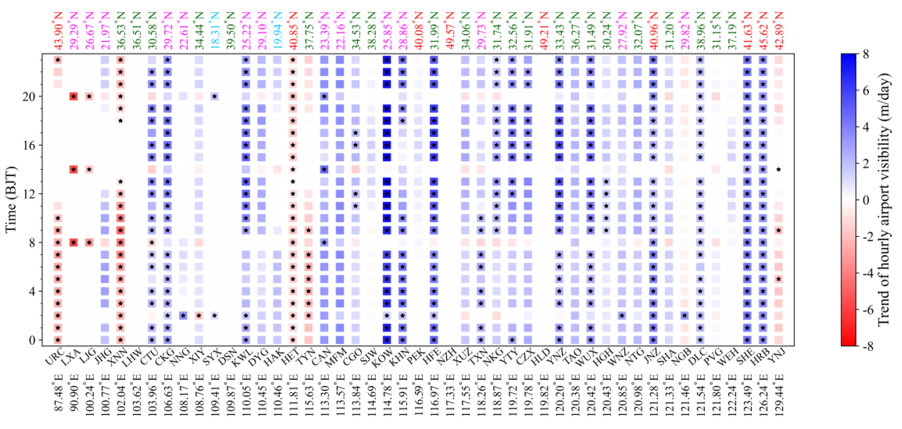
3.2. Diurnal Mean and Trends of Hourly Airport Visibility

Hourly mean visibility during 2010–2020 ranges from 6.5 km at 7:00 a.m. Beijing Time (The following times are all Beijing time) at XUZ in Xuzhou to 40.8 km at 14:00 p.m. at LXA (Figure 5).
For all airports, good visibility mainly occurs between 14:00–18:00 p.m., while poor visibility mainly concentrates from 22:00 p.m. to 12:00 p.m. the next day, especially between 3:00–9:00 a.m. It can be seen that the visibility of the airport is the poorest in the early morning and morning. In the early morning and morning, poorest visibility occurs at CTU (in Chengdu), XIY (in Xian), DYG (in Zhangjiajie), XUZ (in Xuzhou) and HGH (in Hangzhou), which concentrate between 29° N and 35° N. Within the same longitude range, airports with latitude more than 40° N have better visibility, such as HET, NZH and HLD located in 110° N–120° N, and JNZ, SHE and HRB located in 121° N–130° N.
The trends of hourly visibility during 2010–2020 range from –5.81 m/day at 20:00 p.m. at LXA to 7.81 m/day at 12:00 p.m. at KOW in Ganzhou (Figure 6).
The visibility at most airports shows a positive trend at most times. Similar to Figure 4, the increasing visibility mainly occurs in most international airports of China, while decreasing visibility mainly appears in the western and northern parts of China. KOW, KHN (in Nanchang), HFE (in Hefei), SHE (in Shenyang) and HRB (in Harbin) own the greatest and most significant positive trends during all day, while the greatest and most significant negative trends can be found at XNN (in Xining), URC, HET (in Hohhot), LXA and LJG (in Lijiang). In several airports showing a negative trend of visibility (e.g., URC, XNN, TYN and YNJ), the visibility during 14:00–17:00 p.m. has not changed, and the negative trend mainly appears in other times except this time period. Although LXA has the most significant visibility negative trend, unlike most other airports visibility with negative trend (e.g., XNN, URC and HET), LXA has a significant negative trend at only three times (8:00 a.m., 14:00 p.m. and 20:00 p.m.), and there is basically no change in other times. LJG also has the same visibility variation situation. The hours of 8:00 a.m., 14:00 p.m. and 20:00 p.m. are special for visibility at all airports. Compared with the visibility at different times at the same airport, the visibility at these above three times shows opposite or small changes in some airports. On the whole, the hourly visibility changes are the same in a day, showing the same increase and decrease.

3.3. Model Training and Testing

All hourly samples of 26 meteorological elements in 2018–2019 are used to train airport visibility estimation models proposed in this study. Except for LAR, most models are universal to all airports and perform well, and obtain mean Spearman correlation coefficient (CC) values of 0.75, 0.91, 0.96, 0.90, 0.97, 0.91, 0.88 and 0.90 for the PLS-, CART-, KNN-, MLP-, RF-, RR-, SGD- and SVR-based models, respectively (Figure 7).
Except that the standard deviation ratios between standard deviations of the predicted and observed of LAR and SVR methods is discrete around 1, the ratios of other models are concentrated around 1, which shows that most models are well trained and universal for all international airports. In general, RF show the better estimation results from the root mean square error (RMSE) and the mean absolute error (MAE) (Figure 8).
To validate and compare the ability of our proposed airport visibility estimation models in the training period (2018–2019), hourly airport visibility estimates in 2020 are benchmarked against in situ airport visibility measurements in 2020. Figure 9 and Figure 10 show the comparison results (the standard deviation ratio, CC, MAE and RMSE) of the hourly predicted and observed airports visibility in the testing period (2020) for RF-, RR-, LAR-, SVR-, KNN-, SGD-, PLS-, CART-, and MLP-based models. Compared with the results of algorithm-based models in the training period, though the CC values of validation results of these three models show slight reduction to some extent, the CC value at most airports for most algorithms can still be higher than 0.5, which shows that the prediction results are still satisfactory (Figure 7 and Figure 9). In the verification results, HFE (in Hefei), XIY (in Xian), SJW (in Shijiazhuang), TYN (in Taiyuan), NKG (in Nanjing) and YTY (in Yangzhou) have the highest average CC values in algorithm models, which indicates that various models can be well applied in the visibility prediction at these airports. Meanwhile, the average CC values of 29 airports (61.7% of all 47 airports) are more than 0.8, which shows that our proposed artificial intelligence algorithm models can be reasonably used in airport visibility prediction. In particular, HFE and SJW have the highest CC values and high standard deviation ratios in most algorithm models. On the contrary, the lowest CC values of the prediction models appear at LXA and LHW (in Lanzhou) airports.
The standard deviation ratios of most airports under CART, KNN, MLP, RF, RR and SGD are close to 1, indicating that under these algorithms, the dispersion degrees of predicted and observed visibility are close (Figure 9).
If the standard deviation ratios are dispersed around 1, it means that there is a great difference in the dispersion between the predicted and observed under these algorithms, e.g., LAR and SVR. Under the RF-based model, the CC values at most airport visibility are the highest, and there is the closest degree of dispersion between the predicted and observed. Therefore, the RF-based model has the best prediction effect among several algorithm models. The above description can also be seen from the RMSE and MAE values of each month; that is, RF has the best effect (the lowest RMSE and MAE in all months) (Figure 10). RMSE and MAE are higher in May–September and lower in October–December, indicating that the forecast results of visibility in May–September are worse and in October–December are better than those in other months.
In general, the prediction results of the nine algorithm-based models for airport visibility from October to December are better than those in other months, and the prediction results in May–September are poor. Among the algorithm models, the prediction performance of the RF-based model is the best.

4. Discussions

4.1. Distributions and Changes of Airport Visibility in Different Time Scales

Scholars pointed out that relative humidity, suspended particles, and wind speed are closely related to airport visibility [55,56,57,58]. Particles are composed of liquids or solids and are collectively referred to as particulate matter (PM). PM emissions at the airports mainly come from aircraft engines, especially under high thrust conditions such as take-off, climb and cruise. Although individual sources of PM seem to disappear when it diffuses in the atmosphere, it does not disappear, but is diluted. In this process, different plumes from different sources fuse into an uncharacteristic and uniform smoke, which affects the visibility of the airport [59]. On the other hand, as most inorganic salts are hygroscopic, the water vapor attached to the suspended particles in the air will form droplets. With the increase of relative humidity in the atmosphere, the suspended particles in the air will absorb more water vapor and then their particle size will grow by colliding and merging, so as to increase the extinction coefficient and cause the phenomenon of low visibility [55,56]. In addition, the stable near ground inversion or isothermal stratification makes it difficult for water vapor and condensate to diffuse to high altitude or transport to other areas through turbulence, which is conducive to the generation and maintenance of low visibility. The increase of airport water vapor in the lower troposphere caused by aircraft may also have a secondary impact on visibility and some microphysical processes [60]. The lower wind speed makes the turbulence mixing intensity over the airport smaller, which makes it easier to maintain and generate fog and smoke, and not easy to dissipate. In cold seasons, lower ground wind speed is required for low visibility, while in warm seasons with active warm moisture flow, windy weather with heavy precipitation may also cause low visibility [58]. However, after calculating the Spearman correlation coefficients between hourly visibility and 27 meteorological elements during 2018–2020, we found that the correlations between visibility and meteorological elements were not significant at all airports (results not shown). This shows that although some meteorological elements have more important contributions to airport visibility, the change of visibility is affected by the more complex comprehensive action of various factors, and a single factor cannot quantitatively characterize the visibility characteristics.
The probability of low visibility at airports is the highest in the early morning and is the lowest in the afternoon, which has been supported by scholars [58]. The visibility decreases rapidly from afternoon to dusk, which may be mainly due to the small specific heat capacity of the ground environment after the sun sets, resulting in the rapid reduction of temperature, the reduction of temperature dew point difference, and then the condensation of water vapor and the increase of relative humidity, resulting in the low visibility.
Similar to the studies [59,61], in terms of monthly distribution, all airports have low visibility in winter and spring and high visibility in summer and autumn. This is mainly due to the stable atmospheric stratification in winter, which is not conducive to the diffusion of pollutants, while there are many convective weather and rain in summer and autumn, which is conducive to the settlement and removal of pollutants. Due to the large dependence on fossil fuels in cold seasons, the air pollution in northern China is more serious than that in southern China, especially in Beijing, Tianjin and Hebei, central and Southern Hebei, Shandong and Shanxi [62]. This corresponds to our research results; that is, the visibility in the above areas is apparently poorer than in other northern regions, and the visibility in winter is poorer than in summer.
In our study, we found that the visibility at LXA (in Lhasa), XNN (in Xining) and URC (in Urumqi) located in the dry western China have decreased in recent decades, which may be related to the change of wind speed in these areas in recent decades. Mahowald et al. [63] pointed out that there is a high correlation between wind and visibility in China’s arid and semi-arid regions, because the wind drives the change of sand and dust in this region to a great extent. Combined with the study that wind speed on Lhasa and Xining showing positive trends in recent years [29], it can be concluded that the negative trend of visibility in Lhasa and Xining in recent decades is due to the increase of dust weather caused by the increase of wind speed.

4.2. Prediction Performances of Different Models

By comparing nine algorithm models for predicting hourly airport visibility, we find that the RF-based model performs best. The good prediction performance, the ability to deal with continuous variables and classified variables, the characteristics of not over fitting data and the ability to reduce deviation of the RF-based model should be the reasons for the best prediction results [42,54,55,56,57,58,59,60,61,62,63,64,65]. So, due to getting more accurate prediction results without special parameter setting, RF method has better generalization ability, and is a reliable method more suitable for practical application.
SVR is sensitive to the choice of parameters and kernel functions. The performance of SVR mainly depends on the selection of kernel function. Therefore, for the practical problems such as predicting visibility, selecting the appropriate kernel function according to the data models of different airports and constructing SVM algorithm may be an effective way to improve the prediction results. Thererfore, using the same kernel function at different airports may cause great differences in the prediction results of different airports. However, when selecting different forms of kernel functions and parameters in different airports, it is necessary to introduce more comprehensive knowledge of climate, atmospheric environment, and underlying surface characteristics, which is still a very difficult practical problem at present.
One of the advantages of KNN is that it can have good performance without too much adjustment. Before considering using more advanced technology, trying the KNN-based model is a good benchmark method. However, for algorithmic models such as KNN and CART, data preprocessing is very important. If the calculation speed is properly abandoned and preprocessing steps such as data normalization are increased, the prediction accuracy may be improved.

5. Conclusions

In this study, the hourly visibility data from weather stations during 2010–2020 are employed to investigate visibility and its changes at monthly and annual time scales at 47 international airports in China, and the hourly visibility data during 2018–2020 are used to train and test the visibility prediction model. The major findings are summarized as follows.
  • The visibility of airports in eastern and central China is at a poor level all year round, and LXA has good visibility all year round. Airports in south and northwest China have better visibility from May to October and poorer visibility from November to April.
  • In all months, the increasing visibility mainly occurs in the central, northeast and coastal areas of China, while decreasing visibility mainly appears in the western and northern parts of China. In spring, summer and autumn, the changes difference between east and west is particularly obvious. This East–West distribution of trends is obviously different from the North–South distribution shown by the mean.
  • For all airports, good visibility mainly occurs from 14:00–18:00 p.m., while poor visibility mainly concentrates from 22:00 p.m. to 12:00 p.m. the next day, especially between 3:00–9:00 a.m.
  • Our proposed artificial intelligence algorithm models can be reasonably used in airport visibility prediction. In particular, most algorithm models have the best results in the visibility prediction over HFE (in Hefei) and SJW (in Shijiazhuang). On the contrary, the worst forecast results appear at LXA and LHW (in Lanzhou) airports. The prediction results of airport visibility in cold seasons (October–December) are better than those in warm seasons (May–September). Among the algorithm models, the prediction performance of the RF-based model is the best.
There is little research on the temporal and spatial characteristics of airport visibility in China, which is an innovation of this study. Moreover, it is a great contribution to the industry to systematically predict the hourly visibility of an airport with a machine learning model. For the analysis and prediction of the influencing factors of airport visibility, there are still some contents that can be further studied. For example, airport visibility depends not only on meteorological conditions, but also on the light intensity and background light of the airport runway. In addition, in terms of methods, new artificial intelligence methods are developing rapidly, and algorithms such as the graph convolution network may be improved in the future. Therefore, future research work will focus on finding a more relevant relationship between visibility and its influencing factors, and developing new methods to further obtain more accurate prediction results. On the other hand, in our research, only meteorological elements are used as input data, which can quickly complete the data preprocessing and effectively improve the calculation speed of the algorithm, but this may also be a limitation. It is also worth considering adding multiple data such as mode output elements and satellites as inputs to try to obtain higher accuracy. Airports outside China have not been considered at present. Due to the limitations and the acquisition of meteorological data, it can be considered to try and promote this in the future.

Author Contributions

Writing—original draft, J.D.; Writing—review and editing, J.D.; Supervision, G.Z., J.Y. and X.Z.; Data curation, S.W., B.X., J.G., R.J. and K.W.; Methodology, G.Z.; Visualization, J.D. All authors have read and agreed to the published version of the manuscript.

Funding

This study is supported by the National Key Research and Development program of China (2020YFB1600103) and the National Natural Science Foundation of China (grants 41871020).

Acknowledgments

This study is supported by the National Key Research and Development program of China (2020YFB1600103) and the National Natural Science Foundation of China (grants 41871020). We also thank the reviewers and editors for their valuable suggestions for this study.

Conflicts of Interest

The authors declare no conflict of interest.

References

  1. Kneringer, P.; Dietz, S.J.; Mayr, G.J.; Zeileis, A. Probabilistic Nowcasting of Low-Visibility Procedure States at Vienna International Airport During Cold Season. Pure Appl. Geophys. 2018, 176, 2165–2177. [Google Scholar] [CrossRef] [Green Version]
  2. Liu, D.; Jiang, T.; Zhang, Y.; Wang, Y.; Pan, X.; Wu, J. Forecast model of airport haze visibility and meteorological factors based on SVR-RBF model. IOP Conf. Ser. Earth Environ. Sci. 2021, 657, 012029. [Google Scholar] [CrossRef]
  3. Abbey, D.E.; Ostro, B.E.; Fraser, G.; Vancuren, T.; Burchette, R.J. Estimating fine particulates less than 2.5 microns in aerodynamic diameter (pm2.5) from airport visibility data in california. J. Expo. Anal. Environ. Epidemiol. 1995, 5, 161–180. [Google Scholar] [CrossRef] [PubMed]
  4. Iwakura, S.; Okada, K. Dependence of Prevailing Visibility on Relative Humidity at Tokyo International Airport. Pap. Meteorol. Geophys. 1999, 50, 81–90. [Google Scholar] [CrossRef]
  5. Shu, Z.; Yang, S.; Xu, W. The System of the Calibration for Visibility Measurement Instrument Under the Atmospheric Aerosol Simulation Environment. EPJ Web Conf. 2016, 119, 23005. [Google Scholar] [CrossRef] [Green Version]
  6. Won, W.-S.; Oh, R.; Lee, W.; Kim, K.-Y.; Ku, S.; Su, P.-C.; Yoon, Y.-J. Impact of Fine Particulate Matter on Visibility at Incheon International Airport, South Korea. Aerosol Air Qual. Res. 2020, 20, 1048–1061. [Google Scholar] [CrossRef] [Green Version]
  7. Wei, G.; Zhang, Z.; Ouyang, X.; Shen, Y.; Jiang, S.; Liu, B.; He, B.-J. Delineating the spatial-temporal variation of air pollution with urbanization in the Belt and Road Initiative area. Environ. Impact Assess. Rev. 2021, 91, 106646. [Google Scholar] [CrossRef]
  8. França, G.B.; Carmo, L.F.R.D.; De Almeida, M.V.; Neto, F.L.A. Fog at the Guarulhos International Airport from 1951 to 2015. Pure Appl. Geophys. 2018, 176, 2191–2202. [Google Scholar] [CrossRef]
  9. Kutty, S.G.; Agnihotri, G.; Dimri, A.P.; Gultepe, I. Fog Occurrence and Associated Meteorological Factors Over Kempegowda International Airport, India. Pure Appl. Geophys. 2018, 176, 2179–2190. [Google Scholar] [CrossRef]
  10. Dutta, D.; Chaudhuri, S. Nowcasting visibility during wintertime fog over the airport of a metropolis of India: Decision tree algorithm and artificial neural network approach. Nat. Hazards 2015, 75, 1349–1368. [Google Scholar] [CrossRef]
  11. Zhu, L.; Zhu, G.; Han, L.; Wang, N. The Application of Deep Learning in Airport Visibility Forecast. Atmos. Clim. Sci. 2017, 7, 314–322. [Google Scholar] [CrossRef] [Green Version]
  12. Oğuz, K.; Pekin, M.A. Predictability of fog visibility with artificial neural network for esenboga airport. Eur. J. Sci. Technol. 2019, 15, 542–551. [Google Scholar] [CrossRef] [Green Version]
  13. Goswami, S.; Chaudhuri, S.; Das, D.; Sarkar, I.; Basu, D. Adaptive neuro-fuzzy inference system to estimate the predictability of visibility during fog over Delhi, India. Meteorol. Appl. 2020, 27, e1900. [Google Scholar] [CrossRef]
  14. Cornejo-Bueno, S.; Casillas-Pérez, D.; Cornejo-Bueno, L.; Chidean, M.I.; Caamaño, A.J.; Sanz-Justo, J.; Casanova-Mateo, C.; Salcedo-Sanz, S. Persistence Analysis and Prediction of Low-Visibility Events at Valladolid Airport, Spain. Symmetry 2020, 12, 1045. [Google Scholar] [CrossRef]
  15. Marzban, C.; Leyton, S.; Colman, B. Ceiling and Visibility Forecasts via Neural Networks. Weather. Forecast. 2007, 22, 466–479. [Google Scholar] [CrossRef] [Green Version]
  16. Fabbian, D.; de Dear, R.; Lellyett, S.C. Application of Artificial Neural Network Forecasts to Predict Fog at Canberra International Airport. Weather. Forecast. 2007, 22, 372–381. [Google Scholar] [CrossRef]
  17. Mann, H.B. Nonparametric tests against trend. Econometrica 1945, 13, 245–259. [Google Scholar] [CrossRef]
  18. Kendall, M.G. Rank Correlation Methods; Griffin: London, UK, 1975. [Google Scholar]
  19. Sen, P.K. Estimates of the regression coefficient based on Kendall’s Tau. J. Am. Stat. Assoc. 1968, 63, 1379–1389. [Google Scholar] [CrossRef]
  20. Ghalhari, G.F.; Dastjerdi, J.K.; Nokhandan, M.H. Using Mann Kendal and t-test methods in identifying trends of climatic elements: A case study of northern parts of Iran. Manag. Sci. Lett. 2012, 2, 911–920. [Google Scholar] [CrossRef]
  21. Rehman, S. Long-Term Wind Speed Analysis and Detection of its Trends Using Mann–Kendall Test and Linear Regression Method. Arab. J. Sci. Eng. 2012, 38, 421–437. [Google Scholar] [CrossRef]
  22. Tekleab, S.; Mohamed, Y.; Uhlenbrook, S. Hydro-climatic trends in the Abay/Upper Blue Nile basin, Ethiopia. Phys. Chem. Earth Parts A/B/C 2013, 61–62, 32–42. [Google Scholar] [CrossRef]
  23. Sa’Adi, Z.; Shahid, S.; Ismail, T.; Chung, E.-S.; Wang, X.-J. Trends analysis of rainfall and rainfall extremes in Sarawak, Malaysia using modified Mann–Kendall test. Theor. Appl. Clim. 2017, 131, 263–277. [Google Scholar] [CrossRef]
  24. Elnesr, M.N.; Alazba, A.A. Seasonal trends of air temperature and diurnal range in the Arabian Peninsula, the Levant, and Iraq: A spatiotemporal study and development of an online data visualization tool. Theor. Appl. Climatol. 2019, 137, 1271–1287. [Google Scholar] [CrossRef]
  25. Serencam, U. Innovative trend analysis of total annual rainfall and temperature variability case study: Yesilirmak region, Turkey. Arab. J. Geosci. 2019, 12, 704. [Google Scholar] [CrossRef]
  26. Dinpashoh, Y.; Babamiri, O. Trends in reference crop evapotranspiration in Urmia Lake basin. Arab. J. Geosci. 2020, 13, 372. [Google Scholar] [CrossRef]
  27. de Jesus, A.L.; Thompson, H.; Knibbs, L.D.; Hanigan, I.; De Torres, L.; Fisher, G.; Berko, H.; Morawska, L. Two decades of trends in urban particulate matter concentrations across Australia. Environ. Res. 2020, 190, 110021. [Google Scholar] [CrossRef]
  28. Mallick, J.; Talukdar, S.; Alsubih, M.; Salam, R.; Ahmed, M.; Ben Kahla, N.; Shamimuzzaman, M. Analysing the trend of rainfall in Asir region of Saudi Arabia using the family of Mann-Kendall tests, innovative trend analysis, and detrended fluctuation analysis. Theor. Appl. Clim. 2021, 143, 823–841. [Google Scholar] [CrossRef]
  29. Ding, J.; Cuo, L.; Zhang, Y.; Zhang, C. Varied spatiotemporal changes in wind speed over the Tibetan Plateau and its surroundings in the past decades. Int. J. Clim. 2021, 41, 5956–5976. [Google Scholar] [CrossRef]
  30. Ding, J.; Cuo, L.; Zhang, Y.; Zhang, C.; Liang, L.; Liu, Z. Annual and Seasonal Precipitation and Their Extremes over the Tibetan Plateau and Its Surroundings in 1963–2015. Atmosphere 2021, 12, 620. [Google Scholar] [CrossRef]
  31. Zheng, X.B.; Zhao, T.L.; Luo, Y.X.; Duan, C.C.; Chen, J. Trends in sunshine duration and atmospheric visibility in the yunnan-guizhou plateau, 1961–2015. Sci. Cold Arid. Reg. 2011, 3, 179–184. [Google Scholar] [CrossRef]
  32. Araghi, A.; Mousavi-Baygi, M.; Adamowski, J.; Martinez, C.J. Analyzing trends of days with low atmospheric visibility in Iran during 1968–2013. Environ. Monit. Assess. 2019, 191, 249. [Google Scholar] [CrossRef]
  33. Alhathloul, S.H.; Khan, A.A.; Mishra, A.K. Trend analysis and change point detection of annual and seasonal horizontal visibility trends in Saudi Arabia. Theor. Appl. Clim. 2021, 144, 127–146. [Google Scholar] [CrossRef]
  34. Ding, J.; Cuo, L.; Zhang, Y.; Zhu, F. Monthly and annual temperature extremes and their changes on the Tibetan Plateau and its surroundings during 1963–2015. Sci. Rep. 2018, 8, 11860. [Google Scholar] [CrossRef] [Green Version]
  35. Zhang, Z. Research on Spatial and Temporal Variation Characteristics, Factors, and Source Apportionment of PM2. Master’s Thesis, Zhejiang University, Hangzhou, China, 2014. (In Chinese). [Google Scholar]
  36. Shi, D.; Li, C.; Shi, Y.; Zhang, Y. Study on the localization diagnosis of extra heavy fog on the background of the fog weather based on machine learning algorithms. J. Catastrophol. 2018, 33, 193–199. [Google Scholar] [CrossRef]
  37. Xie, Y. Deep Learning Architectures for PM2.5 and Visibility Predictions. Master’s Thesis, The Delft University of Technology, Delft, The Netherlands, 2018. [Google Scholar]
  38. Feng, R.; Gao, H.; Luo, K.; Fan, J.-R. Analysis and accurate prediction of ambient PM2.5 in China using Multi-layer Perceptron. Atmos. Environ. 2020, 232, 117534. [Google Scholar] [CrossRef]
  39. Li, J.; Garshick, E.; Hart, J.E.; Li, L.; Shi, L.; Al-Hemoud, A.; Huang, S.; Koutrakis, P. Estimation of ambient PM2.5 in Iraq and Kuwait from 2001 to 2018 using machine learning and remote sensing. Environ. Int. 2021, 151, 106445. [Google Scholar] [CrossRef]
  40. Shogrkhodaei, S.Z.; Razavi-Termeh, S.V.; Fathnia, A. Spatio-temporal modeling of PM2.5 risk mapping using three machine learning algorithms. Environ. Pollut. 2021, 289, 117859. [Google Scholar] [CrossRef] [PubMed]
  41. Avila, J.; Hauck, T. Least angle regression. Ann. Stat. 2004, 32, 407–499. [Google Scholar] [CrossRef] [Green Version]
  42. Breiman, L. Random Forests. Mach. Learn. 2001, 45, 5–32. [Google Scholar] [CrossRef] [Green Version]
  43. Calle, M.L.; Urrea, V. Letter to the Editor: Stability of Random Forest importance measures. Brief. Bioinform. 2011, 12, 86–89. [Google Scholar] [CrossRef] [PubMed] [Green Version]
  44. Micheletti, N.; Foresti, L.; Robert, S.; Leuenberger, M.; Pedrazzini, A.; Jaboyedoff, M.; Kanevski, M. Machine Learning Feature Selection Methods for Landslide Susceptibility Mapping. Math. Geosci. 2014, 46, 33–57. [Google Scholar] [CrossRef] [Green Version]
  45. Pham, Q.B.; Mukherjee, K.; Norouzi, A.; Linh, N.T.T.; Janizadeh, S.; Ahmadi, K.; Cerdà, A.; Doan, T.N.C.; Anh, D.T. Head-cut gully erosion susceptibility modelling based on ensemble Random Forest with oblique decision trees in Fareghan watershed, Iran. Geomat. Nat. Hazards Risk 2020, 11, 2385–2410. [Google Scholar] [CrossRef]
  46. Abu El-Magd, S.A.; Ali, S.A.; Pham, Q.B. Spatial modeling and susceptibility zonation of landslides using random forest, naïve bayes and K-nearest neighbor in a complicated terrain. Earth Sci. Inform. 2021, 14, 1227–1243. [Google Scholar] [CrossRef]
  47. Farebrother, R.W. Further Results on the Mean Square Error of Ridge Regression. J. R. Stat. Soc. Ser. B 1976, 38, 248–250. [Google Scholar] [CrossRef]
  48. Robbins, H.; Monro, S. A Stochastic Approximation Method. Ann. Math. Stat. 1951, 22, 400–407. [Google Scholar] [CrossRef]
  49. Amari, S. A Theory of Adaptive Pattern Classifiers. IEEE Trans. Electron. Comput. 1967, EC-16, 299–307. [Google Scholar] [CrossRef]
  50. Bottou, L. Online Algorithms and Stochastic Approximations. In Online Learning and Neural Networks; Saad, D., Ed.; Cambridge University Press: Cambridge, UK, 1998. [Google Scholar]
  51. Cristianini, N.; Taylor, J.S. An Introduction to Support Vector Machines and Other Kernel-Based Learning Methods; Printed in the United Kingdom at the University Press: Cambridge, UK, 2000. [Google Scholar]
  52. Zhao, D.; Arshad, M.; Wang, J.; Triantafilis, J. Soil exchangeable cations estimation using Vis-NIR spectroscopy in different depths: Effects of multiple calibration models and spiking. Comput. Electron. Agric. 2021, 182, 105990. [Google Scholar] [CrossRef]
  53. Zhao, D.; Li, N.; Zare, E.; Wang, J.; Triantafilis, J. Mapping cation exchange capacity using a quasi-3d joint inversion of EM38 and EM31 data. Soil Tillage Res. 2020, 200, 104618. [Google Scholar] [CrossRef]
  54. Zhao, D.; Zhao, X.; Khongnawang, T.; Arshad, M.; Triantafilis, J. A Vis-NIR Spectral Library to Predict Clay in Australian Cotton Growing Soil. Soil Sci. Soc. Am. J. 2018, 82, 1347–1357. [Google Scholar] [CrossRef]
  55. Yang, J.; Li, Z.; Huang, S. Influence of relative humidity on shortwave radiative properties of atmosphere aerosol particles. Chin. J. Atmos. Sci. 1993, 23, 239–247. (In Chinese) [Google Scholar]
  56. Boudala, F.S.; Isaac, G.A.; Crawford, R.W.; Reid, J. Parameterization of runway visual range as a function of visibility: Implications for numerical weather prediction models. J. Atmos. Ocean. Technol. 2011, 29, 177–191. [Google Scholar] [CrossRef]
  57. Ren, J.; Liu, J.; Li, F.; Cao, X.; Ren, S.; Xu, B.; Zhu, Y. A study of ambient fine particles at Tianjin International Airport, China. Sci. Total Environ. 2016, 556, 126–135. [Google Scholar] [CrossRef] [PubMed]
  58. Yang, Y.; Ding, W. Change Characteristics and Its Influence Mechanism of Low RVR at Shanghai Pudong Airport. J. Arid. Meteorol. 2016, 34, 873–880. (In Chinese) [Google Scholar] [CrossRef]
  59. Chen, J.L.; Qiu, X.; Pan, J.; Bian, Q.G.; Tang, M.; Jiang, F.; Wang, H.M. Analysis of air pollution in shanghai hongqiao airport. Adm. Tech. Environ. Monit. (In Chinese). 2018, 30, 39–43. [Google Scholar] [CrossRef]
  60. Masiol, M.; Harrison, R.M. Aircraft engine exhaust emissions and other airport-related contributions to ambient air pollution: A review. Atmos. Environ. 2014, 95, 409–455. [Google Scholar] [CrossRef] [PubMed] [Green Version]
  61. Liu, P.; Zhang, Y.; Wu, T.; Shen, Z.; Xu, H. Acid-extractable heavy metals in PM2.5 over Xi’an, China: Seasonal distribution and meteorological influence. Environ. Sci. Pollut. Res. 2019, 26, 34357–34367. [Google Scholar] [CrossRef] [PubMed]
  62. Wang, K.; Wang, W.; Li, L.; Li, J.; Wei, L.; Chi, W.; Hong, L.; Zhao, Q.; Jiang, J. Seasonal concentration distribution of PM1.0 and PM2.5 and a risk assessment of bound trace metals in Harbin, China: Effect of the species distribution of heavy metals and heat supply. Sci. Rep. 2020, 10, 8160. [Google Scholar] [CrossRef]
  63. Mahowald, N.M.; Ballantine, J.A.; Feddema, J.; Ramankutty, N. Global trends in visibility: Implications for dust sources. Atmos. Chem. Phys. Discuss. 2007, 7, 3309–3339. [Google Scholar] [CrossRef] [Green Version]
  64. Diaz-Uriarte, R.; Alvarez De Andrés, S. Gene selection and classification of microarray data using random forest. BMC Bioinform. 2006, 7, 3. [Google Scholar] [CrossRef] [PubMed] [Green Version]
  65. Hastie, T.; Tibshirani, R.J.; Friedman, J.H. The elements of statistical learning: Springer. Elements 2009, 1, 267–268. [Google Scholar]
Figure 1. The geographic locations of the international airports in China.
Atmosphere 13 00075 g001
Figure 2. Flowchart of random forest algorithm.
Atmosphere 13 00075 g002
Figure 3. Spatial distributions of monthly and annual visibility during 2010–2020.
Atmosphere 13 00075 g003
Figure 4. Spatial distributions of the trends of monthly and annual visibility during 2010–2020. Triangles represent statistically significant trends (p < 0.05).
Atmosphere 13 00075 g004
Figure 5. Intraday distribution of hourly visibility at 47 international airports during 2010–2020. The airports are arranged left-to-right by longitude along the x-axis. Light blue, pink, dark green and red represent airports located between 10–19° N, 20–29° N, 30–39° N and 40–49° N, respectively.
Atmosphere 13 00075 g005
Figure 6. Trends of hourly visibility intraday distribution of at 47 international airports during 2010–2020. The airports are arranged left-to-right by longitude along the x-axis. Light blue, pink, dark green and red represent airports located between 10–19° N, 20–29° N, 30–39° N and 40–49° N, respectively. Stars represent statistically significant trends (p < 0.05).
Atmosphere 13 00075 g006
Figure 7. Taylor diagram presents a comparison of the hourly predicted and observed airport visibility in the training period (2018–2019). The diagram shows the correlation (the arc coordinate) and ratio of the standard deviation between the hourly predicted and observed (Abscissa and ordinate).
Atmosphere 13 00075 g007
Figure 8. Root mean square error (RMSE) (black box) and mean absolute error (MAE) (blue box) between hourly visibility observations and estimates at 47 airports in the training period (2018–2019). The red solid line and green dotted line represent the median and mean of each algorithm model at 47 airports, respectively. The 25th and 75th percentiles are the bottom and top boundaries of a box, minimum and maximum are the bottom and top whiskers of a box. The notation applies for following box figures.
Atmosphere 13 00075 g008
Figure 9. Taylor diagram presents a comparison of the hourly predicted and observed airports visibility in the testing period (2020). The diagram shows the correlation (the arc coordinate) and ratio of the standard deviation between the hourly predicted and observed (Abscissa and ordinate).
Atmosphere 13 00075 g009
Figure 10. RMSE (black box) and MAE (blue box) between hourly visibility observations and estimates at 47 airports in the testing period (2020).
Atmosphere 13 00075 g010
Table 1. Information of international airports in China.
IDAirport CodeAirport NameCityIDAirport CodeAirport NameCity
1CANBaiyunGuangzhou25NKGLukouNanjing
2CGOXinzhengZhengzhou26NNGWuweiNanning
3CKGJiangbeiChongqing27NTGXingdongNantong
4CTUShuangliuChengdu28NZHXijiaoManzhouli
5CZXBenniuChangzhou29PEKShouduBeijing
6DLCZhoushuiziDalian30PVGPudongShanghai
7DSNYijinhuoluoErdos31SHAHonqiaoShanghai
8DYGHehuaZhangjiajie32SHETaoxianShenyang
9HAKMeilanHaikou33SJWZhengdingShijiazhuang
10HETBaitaHohhot34SYXFenghuangSanya
11HFEXinqiaoHefei35TAOLiutingQingdao
12HGHXiaoshanHangzhou36TXNTunxiHuangshan
13HLDDongshanHailar37TYNWusuTaiyuan
14HRBTaipingHarbin38URCDiwobuUrumqi
15JHGGasaXishuangbanna39WEHDashuipoWeihai
16JNZJinzhouJinzhou40WNZLongwanWenzhou
17KHNChangbeiNanchang41WUHTianheWuhan
18KOWHuangjinGanzhou42XIYXianyangXian
19KWLLiangjiangGuilin43XNNCaojiabuXining
20LHWZhongchuanLanzhou44XUZGuanyinXuzhou
21LJGSanyiLijiang45YNJChaoyangchuanYanji
22LXAGonggaLhasa46YNZNanyangYancheng
23MFMAomenMacao47YTYTaizhouYangzhou
24NGBLisheNingbo
Table 2. Meteorological elements used in this study.
AbbreviationFull Name
visibilityAverage horizontal visibility every 10 min in an hour (m)
TEMAir temperature (°C)
TEM_MinMinimum temperature (°C)
TEM_MaxMaximum temperature (°C)
DPTDew point temperature (°C)
PRSPressure (hPa)
PRS_SeaSea level pressure (hPa)
VAPVapor pressure (hPa)
RHURelative humidity (%)
PRE_1hPrecipitation in the past hour (mm)
PRE_6hPrecipitation in the past 6 h (mm)
PRE_12hPrecipitation in the past 12 h (mm)
GSTGround surface temperature (°C)
GST_5cmGround temperature at 5 cm depth (°C)
GST_10cmGround temperature at 10 cm depth (°C)
GST_15cmGround temperature at 15 cm depth (°C)
GST_20cmGround temperature at 20 cm depth (°C)
WIN_S_Avg_2min2-min average wind speed (m/s)
WIN_S_Avg_10min10-min average wind speed (m/s)
WIN_S_MaxMaximum wind speed (m/s)
WIN_D_S_MaxWind direction of maximum wind speed (degree)
WIN_S_Inst_MaxExtreme instantaneous wind speed (m/s)
WIN_D_Inst_MaxDirection with extreme wind speed (degree)
WIN_S_Inst_Max_6hMaximum instantaneous wind speed in the past 6 h (m/s)
WIN_D_Inst_Max_6hDirection of maximum instantaneous wind speed in the past 6 h (degree)
WIN_S_Inst_Max_12hMaximum instantaneous wind speed in the past 12 h (m/s)
WIN_D_Inst_Max_12hDirection of maximum instantaneous wind speed in the past 12 h (degree)
Publisher’s Note: MDPI stays neutral with regard to jurisdictional claims in published maps and institutional affiliations.

