Article

Solar Radiation Prediction Based on Convolution Neural Network and Long Short-Term Memory

1
College of Mechanical and Electronic Engineering, Nanjing Forestry University, Nanjing 210037, China
2
Key Laboratory of Measurement and Control of Complex Systems of Engineering (Southeast University), Ministry of Education, Nanjing 210096, China
*
Author to whom correspondence should be addressed.
Energies 2021, 14(24), 8498; https://doi.org/10.3390/en14248498
Submission received: 29 October 2021 / Revised: 8 December 2021 / Accepted: 13 December 2021 / Published: 16 December 2021

Abstract

:
Photovoltaic power generation is highly valued and has developed rapidly throughout the world. However, the fluctuation of solar irradiance affects the stability of the photovoltaic power system and endangers the safety of the power grid. Therefore, ultra-short-term solar irradiance predictions are widely used to provide decision support for power dispatching systems. Although a great deal of research has been done, there is still room for improvement regarding the prediction accuracy of solar irradiance including global horizontal irradiance, direct normal irradiance and diffuse irradiance. This study took the direct normal irradiance (DNI) as prediction target and proposed a Siamese convolutional neural network-long short-term memory (SCNN-LSTM) model to predict the inter-hour DNI by combining the time-dependent spatial features of total sky images and historical meteorological observations. First, the features of total sky images were automatically extracted using a Siamese CNN to describe the cloud information. Next, the image features and meteorological observations were fused and then predicted the DNI in 10-min ahead using an LSTM. To verify the validity of the proposed SCNN-LSTM model, several experiments were carried out using two-year historical observation data provided by the National Renewable Energy Laboratory (NREL). The results show that the proposed method achieved nRMSE of 23.47% and forecast skill of 24.51% for the whole year of 2014, and it also did better than some published methods especially under clear sky and rainy days.

Graphical Abstract

1. Introduction

In recent years, under the pressure of global warming, deterioration of the human ecological environment, shortages of non-renewable energy resources, and environmental pollution, solar radiation energy has become highly valued worldwide as an inexhaustible clean energy source, and consequently, solar photovoltaic power has developed rapidly [1,2]. However, photovoltaic power generation is volatile and intermittent, and large-scale grid connections negatively impact the stability and security of the power grid, and even cause serious economic losses [3,4]. In order to increase the proportion of photovoltaic power generation in the power system, the key is to implement timely and effective power dispatching, where accurate photovoltaic power generation forecast is an important basis for the power dispatching process. However, the fluctuation of photovoltaic power generation is mainly caused by changes in solar irradiance. Therefore, it is important to accurately predict solar irradiance, the results of which can provide important decision support for power dispatching systems and can effectively reduce the operational costs of the power system [5,6].
There are many methods used for short-term and ultra-short-term solar irradiance predictions. Traditional prediction methods mainly use statistical methods to establish the relationship between the historical value and solar irradiances, such as time series and regression analysis methods [7,8]. However, traditional statistical methods cannot accurately describe the complex nonlinear relationship between various meteorological variables and the solar irradiance, which limits the improvement of the prediction accuracy.
With the rise of machine learning technology, many scholars have applied machine learning methods into solar irradiance prediction and have achieved good results [9]. For example, support vector machine (SVM) [10], extreme learning machine (ELM) [11], and artificial neural network (ANN) methods [12] have all been shown to produce better results than linear regression prediction methods when predicting solar irradiance. What’s more, machine learning methods, especially ANN, combining with Numerical Weather Prediction are also achieved great improvement on the hour-term or medium-term forecast [13,14,15]. Furthermore, compared to traditional machine learning, deep learning, such as recurrent neural network (RNN), has shown the potential to further improve the prediction of solar irradiance [16].
At the same time, with the development of hardware technologies, such as charge-coupled devices (CCDs), and the continuous improvement of digital image processing technology [17], many total cloud-measuring remote sensing instruments have been successfully developed, such as the total sky imager (TSI), which can accurately monitor and collect cloud images over photovoltaic power stations in real time [18]. The images have sufficient information that is more beneficial to the prediction of solar irradiance than historical observation values, such as cloud cover. However, the existing solar irradiance prediction methods based on the TSI have some disadvantages that cannot be ignored. For example, the artificial image feature extraction relies heavily on the experience of researchers and it is often difficult to obtain satisfactory prediction results [19]. Based on this, Feng et al. [20] designed a SolarNet model that can automatically extract the features of a total sky image, but this model only uses one total sky image as the model input, which ignores the cloud motion information and greatly limits the accuracy of the prediction. Zhao et al. [21] designed a three-dimensional convolutional neural network (3D-CNN) model to realize the fusion of multiple images and historical values, and then input the fusion features into a multilayer perceptron (MLP). However, as a traditional neural network structure, an MLP cannot capture the long-term memory of an input time series because the nodes between the hidden layers are not connected. Therefore, an MLP often performs poorly when predicting a time series. The long short-term memory (LSTM) has a complex memory unit, which can remember the previous information and can apply it to the calculation of the current output, that is, the nodes between hidden layers become connected [22]. Therefore, compared to an MLP, LSTM displays better performance when predicting a time series. In particular, long short-term memory (LSTM) networks have been used to predict solar irradiance due to their strong time series-learning ability [23,24].
Based on the shortcomings of the above model, this study developed a Siamese convolutional neural network-long short-term memory (SCNN–LSTM) model. A Siamese CNN can automatically extract the spatial dimension features of multiple continuous total sky images and can retain the temporal dimension features. Then, historical meteorological features and image features are fused using a concatenate layer, and the fused features are input into the LSTM for the prediction of solar irradiance within hours.
Since the direct normal irradiance (DNI) was vital to the concentrated solar thermal power plant and the global horizontal irradiance was important to photovoltaic solar power plant [25], the DNI was taken as research target in this study to evaluate the performance of the proposed model. The two years’ data were corrected from the National Renewable Energy Laboratory (NREL) [26], and several experiments were carried out to verify the effectiveness of the proposed method.
The main contributions of this study include: (1) A Siamese CNN was developed to automatically extract the features of continuous total sky images, where the Siamese structure reduced the model training time by sharing part parameters of the model; (2) SCNN-LSTM was used to effectively fuse the time-series features of images and meteorological data and to improve the DNI prediction accuracy.
The remainder of this paper is organized as follows: Section 1 introduces the three correlation networks, based on which the proposed model was constructed. Section 2 describes the collection and processing of the experimental materials. Section 3 presents a SCNN–LSTM forecasting model of DNI. Section 4 discusses the experimental results and analyzes the performance of the SCNN–LSTM model based on several comparative experiments. Finally, Section 5 summarizes the conclusions.

2. Data Collection and Preprocessing

2.1. Data Collection

All measured data in the daytime were downloaded from an open database, namely, the NREL’s Solar Radiation Research Laboratory (SRRL) [26]. The SRRL station is located at 39.74 °N and 105.18 °W, 1829 m above sea level in Golden City, Colorado, USA, where there are abundant solar resources. The measured meteorological variables of the SRRL, including the DNI, solar zenith angle, relative humidity, and air mass, are obtained with a 1 min sampling frequency, and the details of these variables are listed in Table 1. There are few negative values of DNI which are very close to zero and are corrected as 0 [27].
The total sky images used were RGB images obtained using the TSI (TSI-880), and the image resolution was 352 × 288 pixels. The total sky images of different weather conditions are shown in Figure 1, where the shadow bands in the image move with the Sun to protect the CCD sensor from direct sunlight. The total sky images are obtained with a 10 min sampling frequency. Therefore, the 10 min averages of the meteorological data were used as the samples in this study. Additionally, the total sky images were removed when the solar zenith angle were greater than 80 degrees in order to avoid hazy sky and obstacle presence [28].

2.2. Data Preprocessing

2.2.1. DNI Clear-Sky Index

In order to eliminate the prediction error caused by the change in solar position, the DNI was converted into a DNI clear sky index by a basic clear sky model [29], which considers the impacts of the atmospheric, seasonal and geographical factors on DNI and calculates the clear-sky DNI with only local time, date and location information. The DNI clear sky index (k) was represented as:
k = I I c l r   ,
where I is the measured value of DNI at a certain moment when it reaches the Earth’s surface, and I c l r is the DNI of theoretical clear sky at the same time when it reaches the Earth’s surface. I c l r is represented as:
I c l r = I s c × ε × τ b   ,
where   I s c is the solar radiation constant 1360.8 W/m2; ε is the eccentricity correction factor, which is the correction factor for the deviation caused by the change in distance between the Sun and the Earth; I s c × ε means the incident solar radiation intensity reaching the top of the Earth’s atmosphere at that moment and τ b is the atmospheric transparency coefficient of the direct irradiance. ε and τ b   are as:
ε 0 = 1 + 0.033 × cos ( 2 π × D O Y 365 ) ,
τ b = 0.7 P L 0.678 ,
where DOY is the day of the year, with counting starting at 1 on New Year’s Day; PL is the ratio of the length of the path of the Sun’s rays through the Earth to the length of the path perpendicular to the zenith angle of the Sun. Its expression is as follows:
P L = ( r + c ) 2 cos 2 ( z ) + ( 2 r + 1 + c ) ( 1 c ) ( r + c ) cos ( z ) ,
where r is the ratio between the Earth’s radius of 6371 km and the effective thickness of the atmosphere of 9 km; c is the ratio between the altitude of the observation site of 1.8288 km and the effective thickness of the atmosphere of 9 km; z is the solar zenith angle which is calculated in radians.

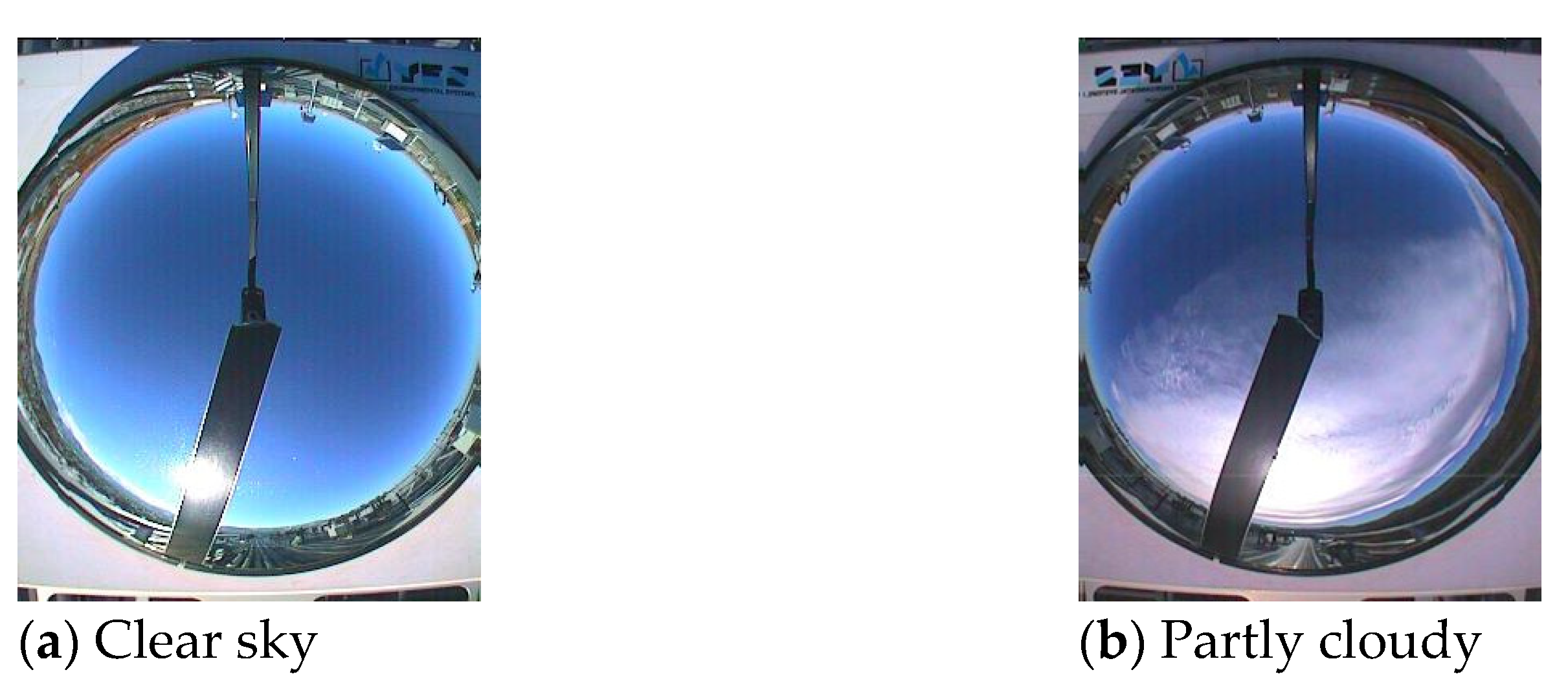
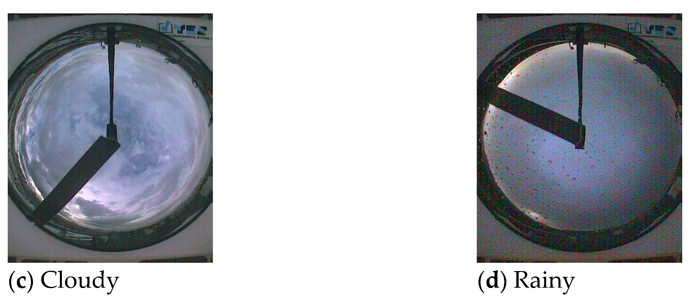
2.2.2. Image Preprocessing

The main task of sky image processing is to extract the region of interest (ROI) out of the RGB image to remove unnecessary pixels. The mask is a binary matrix corresponding to the location of the original foundation cloud map. The pixel value in the mask is either 0 or 1, where 1 corresponds to the location of the sky image in the original foundation cloud map, namely, the ROI, while 0 corresponds to the location of the non-sky image in the original foundation cloud map. The size of the mask image was 352 × 288 and the mask area on it was a circle with a radius of 128 pixels that had the center of the sky as the origin. The original foundation cloud map was multiplied by the mask, and then the extra pixels were cut out to obtain the processed image, as shown in Figure 2c. Finally, a minor gradients algorithm [30] was used to repair the shadow-band pixels as shown in Figure 2d, which was used as the input of the model with a resolution of 256 × 256 pixels.
Finally, the meteorological and image data were collected from 1 January 2013 to 31 December 2014, where a total of 41,139 groups of valid samples were obtained after processing. The data for January and July in the year of 2013 were chosen as the verification set, and the remaining data in the year of 2013 was set as the training set. Meanwhile, the data of the whole year of 2014 were set as the testing set. The details of data segmentation were listed in Table 2.

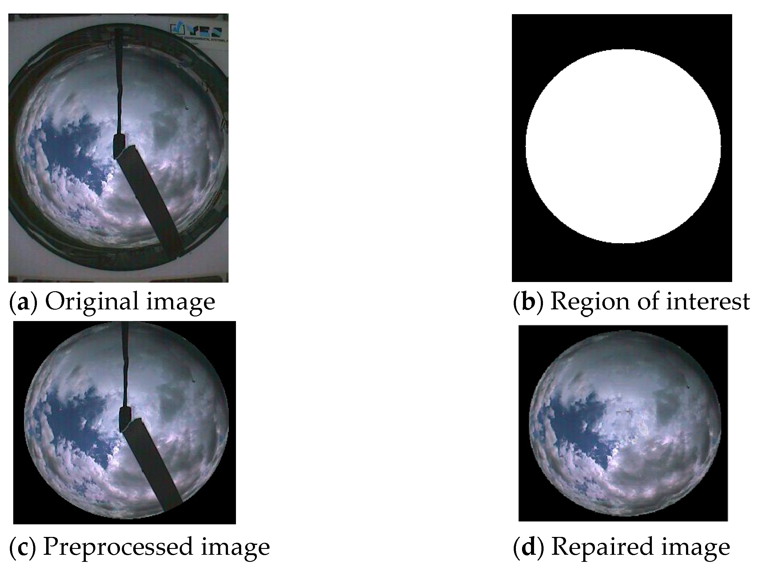
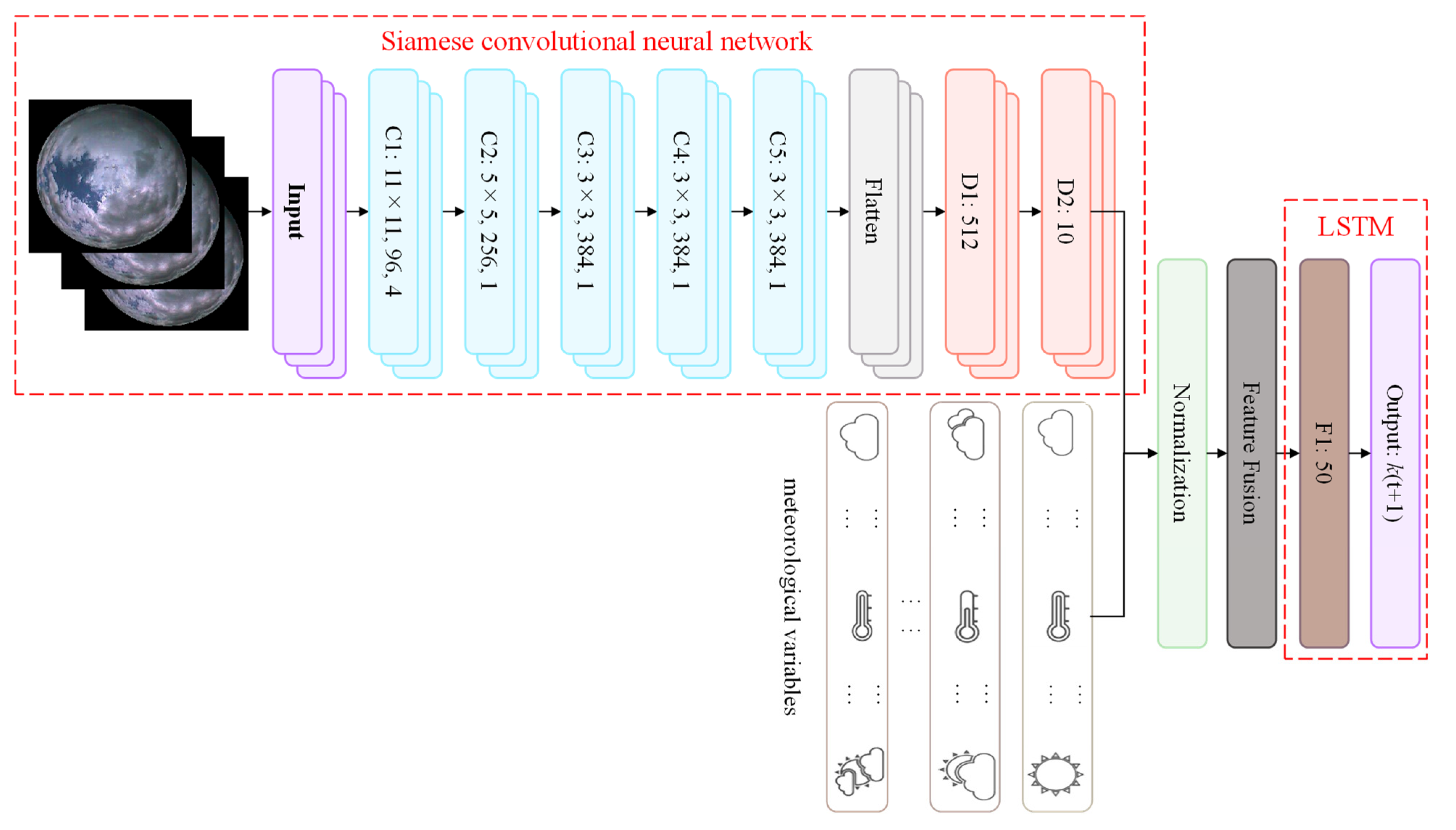
3. SCNN-LSTM Prediction Model

In this section, a SCNN–LSTM model was designed to predict the 10-min ahead DNI, and the structure of SCNN-LSTM model was shown as Figure 3. The cloud features were firstly extracted from a group of consecutive total sky images in order to make up the missing information of a single image blocked by the shadow-band [30,31]; and then the cloud features and meteorological variables were normalized and fused as inputs of LSTM to predict the clear-sky of DNI in the next 10 min.

3.1. Input Dimension

Bayesian information criterion (BIC) was used to determine the input dimension of the forecasting model using DNI clear-sky index; that is, the DNI at moment t was related to the DNI at the previous n moments [32]. The BIC was used to determine the order of the DNI clear sky index sequence after the first-order difference, and the obtained BIC thermal diagram is shown in Figure 4. The BIC information reached the minimum value when the autoregression coefficient was 1 and the moving average coefficient was 2. The DNI clear sky index sequence went through a difference such that the order of the model was determined to be 3, which means that the information at time t − 2Δt, t − Δt, and t predicted the DNI clear sky index at time t + Δt, where Δt is 10 min.

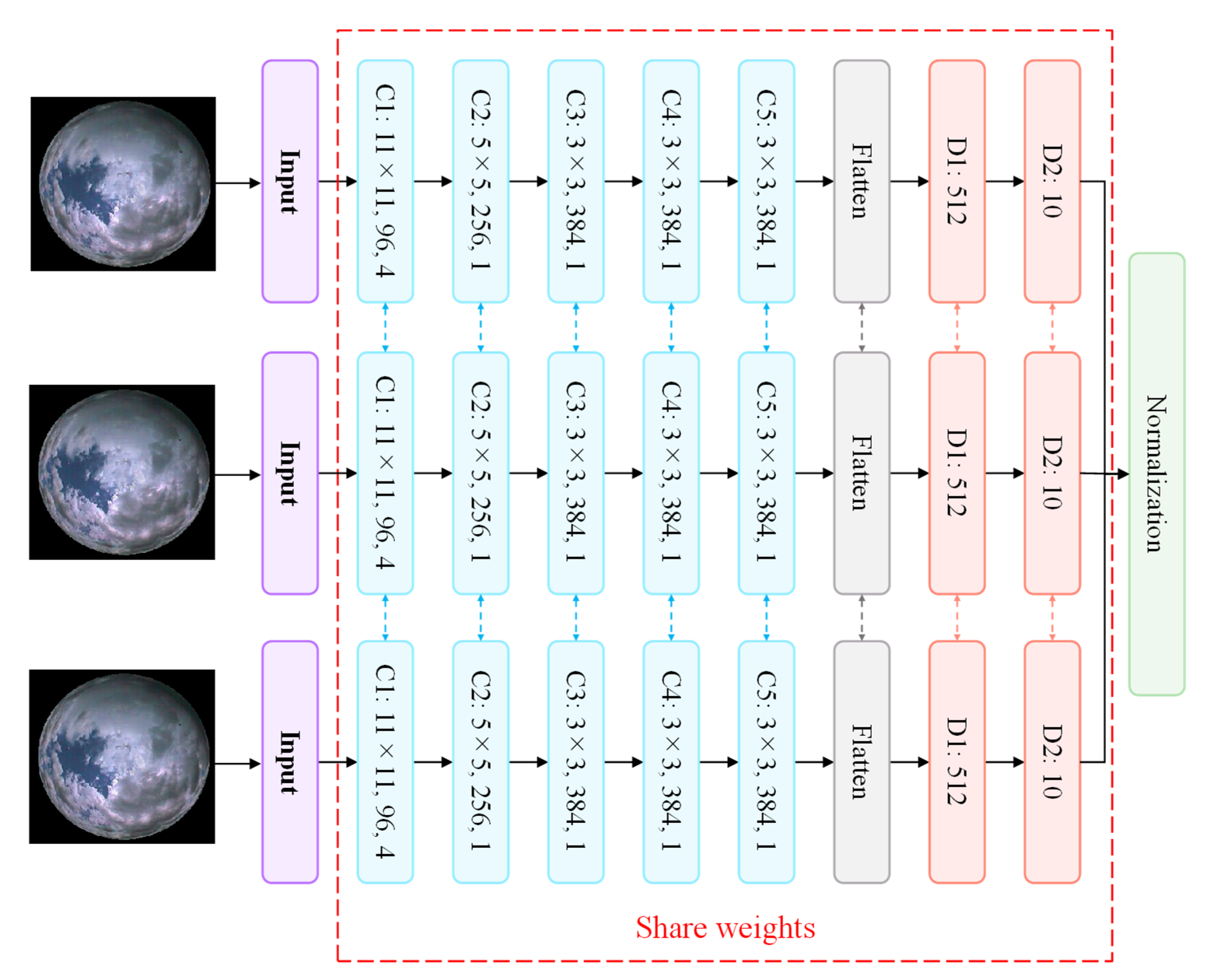
3.2. Siamese Convolutional Neural Network

The convolutional neural network (CNN) is one of the representative algorithms of deep learning. It has the ability of representation learning and is able to extract high-order features from inputs [33]. The main structure of a traditional CNN includes convolutional layers, pooling layers, and fully connected layers. A Siamese network [34] is a class of neural networks that consist of two or more identical subnetworks, and the subnetworks have the same network structure and configuration, including the network parameters and weights. During the training phase, the parameter updates are mirrored across multiple subnetworks.
The proposed Siamese convolution neural network took the advantages of CNN and Siamese network, and it was used to extract the high-order features from ground-based sky images at different times. The branch of the SCNN structure was improved based on the AlexNet network [35]. Because the images of the three input moments (i.e., t − 2Δt, t − Δt, and t) need to be processed, the SCNN has three improved AlexNet subnetworks, and the structure of the SCNN was shown as Figure 5. The network structure, parameters, and weights of the three subnetworks are the same, and the three inputs determine how the weights are updated.

3.3. Long Short-Term Memory

Long short-term memory (LSTM), a variant of a recurrent neural network (RNN), usually performs better than an RNN when predicting outcomes [36]. In LSTM, every neuron is a memory cell and there are three gates in each cell, namely, the forgetting gate f t , the input gate i t , and the output gate o t :
{ f t = σ ( W f [ h t 1 , x t ] + b f ) i t = σ ( W i [ h t 1 , x t ] + b i ) C ˜ t = tan h ( W i [ h t 1 , x t ] + b i ) C t = f t × C t 1 + i t × C ˜ t o t = σ ( W o [ h t 1 , x t ] + b o ) h t = o t × tan h ( C t )   ,
where h t 1 represents the output at the previous moment; x t represents the input at the current moment, and it is the fused features of cloud features and meteorological variables; σ represents the sigmoid function, W represents the weight, and b represents the bias. The process of operation of the whole unit structure decides which information should be discarded in the memory cells of the last moment by multiplying the forgetting gate f t by the previous cell state C t 1 . Then, the new information is obtained by multiplying the input gate i t with the alternative content   C ˜ t that needs to be updated. According to the above system of equations, the cell state C t at the current moment can be obtained by discarding and updating the information. Finally, the C t status value is pushed from −1 to 1 through the tanh layer, and the output h t at the current moment is obtained by multiplying the tanh layer by the output gate o t , which is the DNI clear sky index for the next 10 min; therefore, the DNI at that moment is obtained by multiplying by the predicted clear-sky index by the DNI of the clear sky at the same moment.

3.4. Loss Function

In this study, the greatest difference from a traditional Siamese network is that the SCNN section of the SCNN–LSTM model was designed to find the key features in the total sky images at different times in order to provide the image timing features for the LSTM prediction instead of to compare the similarity between these images. Therefore, there was no need to calculate the Euclidian distance between sample pairs to judge their similarity.
Secondly, the SCNN–LSTM model does not need to use the contrastive loss function to represent the degree of matching between paired samples. Instead, it uses the predicting error (PE) to evaluate the difference between the predicted value and the observed value to train the SCNN–LSTM parameter, as follows:
P E = 1 2 N i = 1 N ( y i y i ) 2 ,
where y i is the predicted value of a forecast model, y i is the target, and N is the number of training samples.
Just as in a traditional Siamese network, the multiple subnetwork branches of the SCNN in this model also have the same network structure, parameters, and weights. In the implementation of the SCNN structure, only one network structure needs to be built, and then the network structure is mirrored to multiple subnetworks with different inputs. All the subnetworks jointly determine how the weights are updated in the network.
During the process of the model training, the weights of the whole model were adjusted simultaneously. First, the PE was used to evaluate the prediction error of the model; then, the error was propagated back to the fully connected layers, the LSTM layer, and the SCNN in turn. Notably, the weight-sharing between the three branches of the SCNN was realized via mirroring, and the weights of the three branches were uniformly determined using the input of the three branches.

4. Results and Discussion

The experimental platform comprised a server containing an Intel Core I9-9900K CPU and a Nvidia GeForce RTX 2080Ti. The SCNN–LSTM model was implemented using the Keras library and Tensorflow.

4.1. Evaluation Index

The correlation coefficients (r), normalized mean bias error (nMBE), normalized mean absolute error (nMAE), and normalized root mean squared error (nRMSE) were used to evaluate the performance of different forecast models, and they are calculated as follows:
r = i = 1 N ( y i y ¯ ) ( y i y ¯ ) i = 1 N ( y i y ¯ ) 2 i = 1 N ( y i y ¯ ) 2 ,
n M B E = 1 N i = 1 N ( y i y i ) / y ¯ × 100 % ,
n M A E = 1 N i = 1 N | y i y i | / y ¯ × 100 % ,  
n R M S E = 1 N i = 1 N ( y i y i ) 2 / y ¯ × 100 % ,
where y i is the predicted value of a forecast model, y ¯ is the mean of all of the predicted values, y i is the target, y ¯ is the mean of all of the targets, and N is the number of testing samples.
Meanwhile, the persistent model is usually used as a benchmark for evaluating the performance of different forecast models and is defined as:
I ( t + 1 ) = I ( t ) .
The evaluating index based on the persistent model, which is called the forecast skill (Fs), is defined as:
F s = ( n R M S E p e r n R M S E f ) / n R M S E p e r × 100 % ,
where n R M S E p e r and n R M S E f are the nRMSEs of the persistent model and the forecast model, respectively.

4.2. Performance of the SCNN-LSTM

The image feature extraction section of the SCNN-LSTM structure was improved using AlexNet. Different numbers of fully connected layers affect the feature extraction outcome; therefore, a group of experiments were conducted to compare three different SCNN-LSTM models with different numbers of fully connected layers in order to obtain an appropriate model structure. The results are listed in Table 3, where Model-1 is a fully connected layer containing 10 neurons following the flatten layer (layer 11), as shown in Figure 5. There were two fully connected layers after the flatten layer in Model-2, which contained 512 and 10 neurons, respectively. Model-3 had three fully connected layers, which contained 512, 256, and 10 neurons, respectively. The results show that the performance of Model-2 was the best among the three models, where its Fs was up to 24.51%.
The LSTM layer of the SCNN-LSTM model was used to process the fusion features for the DNI prediction. Different LSTM layers and the number of neurons affect the prediction performance of the model; therefore, a set of experiments were conducted to select the optimal number of LSTM layers and neurons. The results are listed in Table 4, in which Model-A was the LSTM layer after the feature fusion part (layer 14) as shown in Figure 5, where the number of neurons was 30. The number of neurons in the LSTM layer of Model-B was 50, and Model-C had two LSTM layers containing 50 and 30 neurons, respectively. The results show that the SCNN-LSTM model that adopted an LSTM layer with 50 neurons gave the best prediction effect, had the biggest r and Fs, and had the smallest nMBE, nMAE, and nRMSE.
A group of experiments were carried out by missing an input variable to evaluate its importance for the proposed method, and the results are shown as Figure 6. It is clear that the total sky image is the most important variable for the proposed model, which means that the cloud is the most important variable for the solar radiation. The nRMSE of the proposed method without the solar zenith angle (Z) as inputs is greater than those of predicting models without relative humidity or air mess, which means that the position between the Sun and the observation station is also important for predicting accuracy.

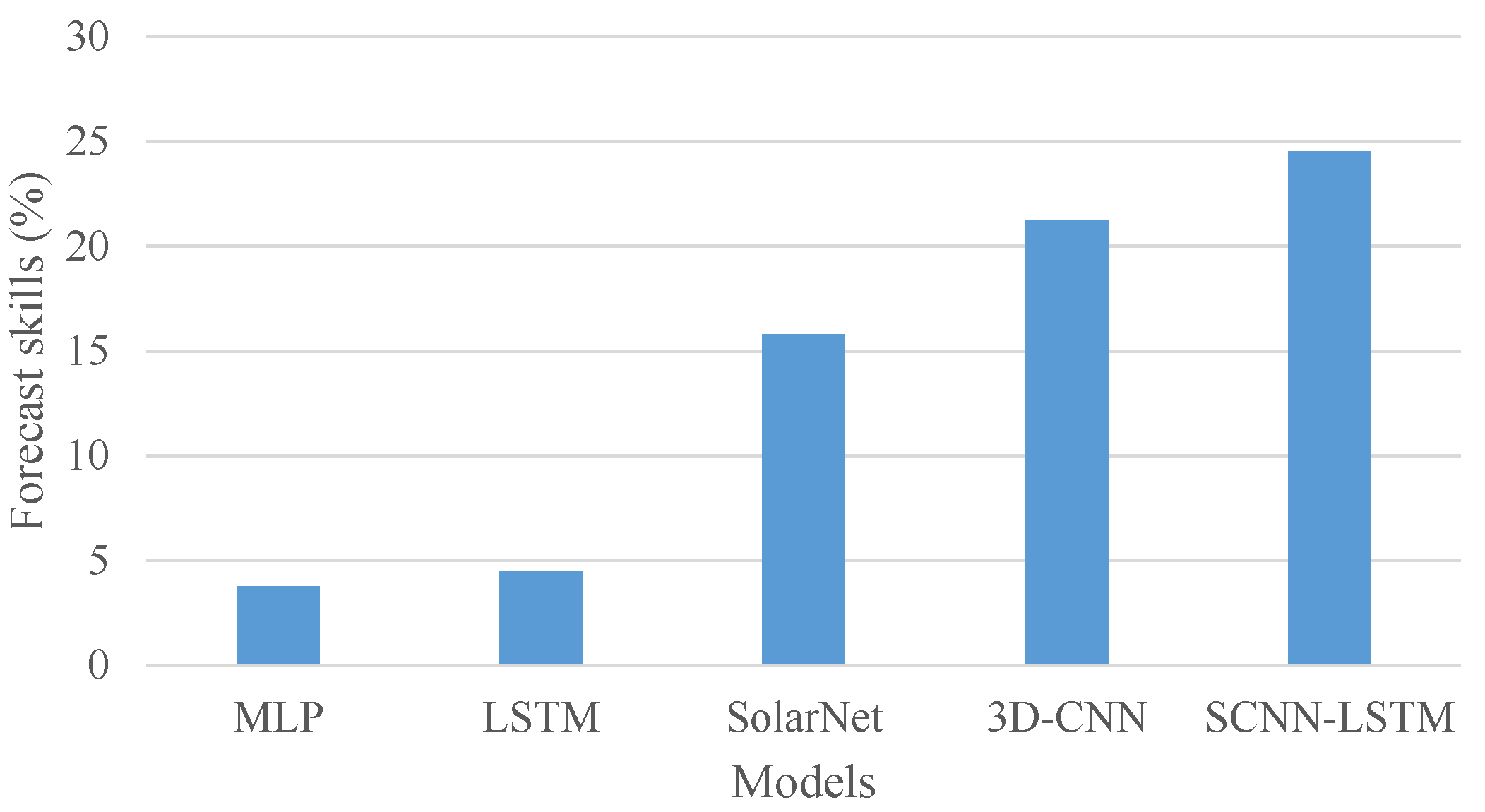
4.3. Performance of Different Forecast Models for the Inter-Hour DNI Forecast

Another group of experiments were carried out to evaluate the performance of the proposed model in comparison to another published method, and the results are listed in Table 5 (Table S1 listed the results of GHI prediction in Supplementary Materials). Among them, the MLP with one hidden layer and LSTM with one layer only used the above meteorological data and cloud cover (instead of total sky images) as the model input, SolarNet only used the total sky images as the model input, and the 3D-CNN and SCNN-LSTM models used the historical observation values and the total sky images as the model input.
It can be seen from Table 5 that the prediction performance was better when using the total sky images as the model input instead of the historical meteorological values. Moreover, the combination of total sky images and historical meteorological values as the model input was able to reach an even better performance than when using them independently. Meanwhile, it can be observed that the nRMSE, nMBE, and nMAE of the SCNN-LSTM model’s predictions were 23.72%, 0.35%, and 13.27%, respectively, which were all lower than the other compared models. Additionally, the correlation coefficient was 0.9592, which was higher than the other compared models, indicating that the SCNN-LSTM model had superior performance regarding DNI prediction 10 min in advance.
In order to make a detailed comparison between the SCNN-LSTM model and the other models, test sets were used to construct error and error cumulative frequency graphs of the observed and predicted values of the DNI. Figure 7 shows that the SCNN-LSTM model improved the accuracy of prediction, mainly by increasing the frequency with a small prediction error and reducing the frequency with a large prediction error.
Figure 8 shows a histogram of the prediction skills of the SCNN-LSTM model and the other comparison models. SolarNet’s prediction skills were significantly higher than those of the MLP and LSTM models, mainly because the total sky images contained more diverse information than the historical observation values, and clouds have a more critical impact on the solar irradiance. The prediction skills of the 3D-CNN and SCNN-LSTM models were superior to those of SolarNet, mainly because a total sky image can better reflect the attenuation degree of radiation from the sky to the ground, and the historical observation value can express the trend of the DNI well. Therefore, the meteorological value and image fusion could be used as the model input to achieve the optimal prediction accuracy. In addition, the prediction skills of the SCNN-LSTM model were better than the 3D-CNN model, mainly because the image feature extraction branch of the SCNN-LSTM model uses an improved AlexNet network. Compared to the 3D-CNN model, the AlexNet network has a greater number of layers and a better image feature extraction effect. At the same time, DNI prediction is a time series prediction. The LSTM in the SCNN-LSTM model has a powerful time series-learning ability; compared to the MLP in the 3D-CNN model, LSTM is more conducive to time series prediction.

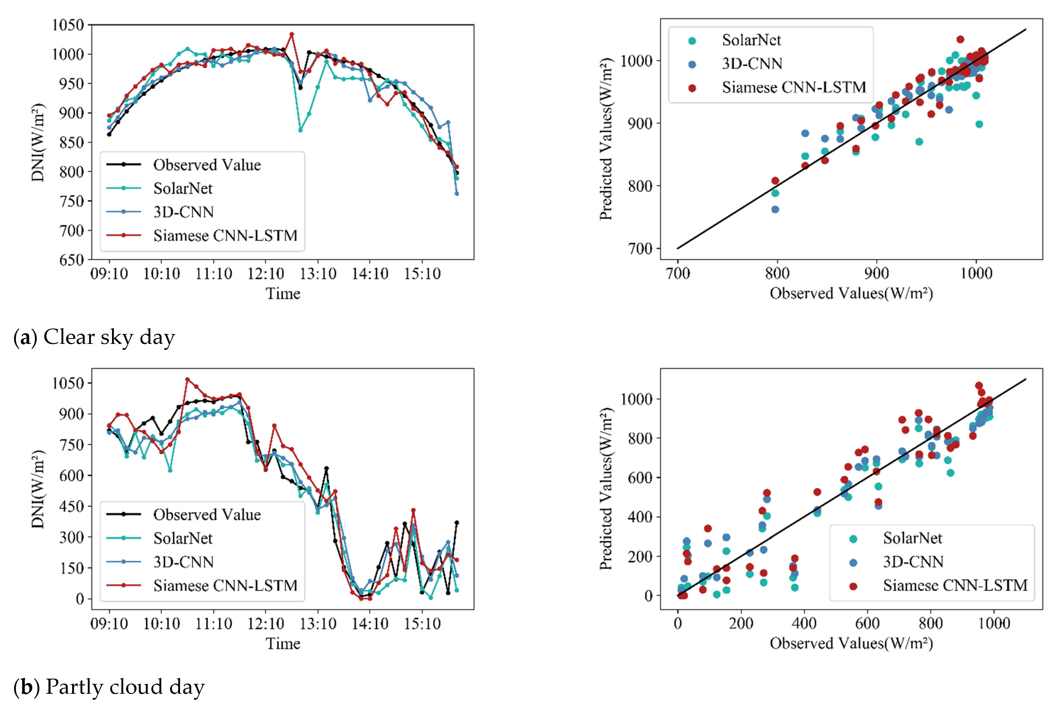
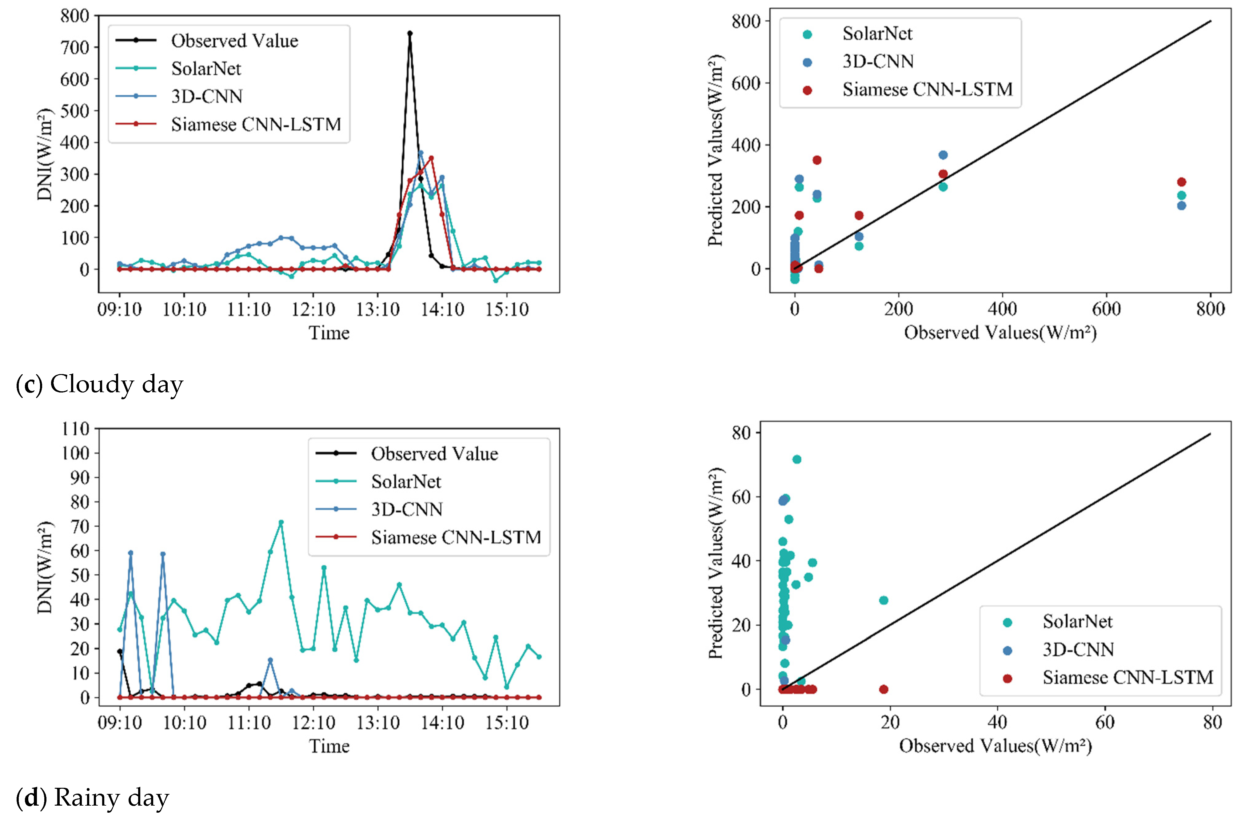
4.4. Performance of Different Forecast Models under Different Weather Conditions

To further analyze the performance of the proposed model, historical data from ten days for every weather condition were selected, and the predicting results were listed in Table 6. The MLP and LSTM without images have similar prediction performance under different weather conditions, and both do worse than the last three deep learning methods with images. The proposed SCNN-LSTM method does best among these methods especially under clear sky and rainy days, and its forecast skills are all greater than 20% under any weather condition.
Historical data from four days with different weather conditions were selected, where Figure 9 shows the performance of the last three models in Table 6, which were all constructed based on a deep CNN with total sky images. For clear sky and partly cloudy days, the fitting effect of the SolarNet, 3D-CNN, and SCNN–LSTM models with the observed value was similar, but for cloudy and rainy days, the SCNN–LSTM model showed a better fitting performance with the observed value. This indicates that compared to the known public model mentioned in this paper, the SCNN–LSTM model can effectively reduce the DNI prediction error for rainy days, which is consistent with the results in Table 6.

5. Conclusions

In this study, a SCNN-LSTM model was proposed for predicting the DNI 10-min ahead. First, a SCNN was built using three component networks by improving the AlexNet network, which independently extracts features from three total sky images and produces the image characteristics at three moments, and the meteorological integration of historical observations. The fusion feature was implemented after the LSTM, and the two fully connected layers output the DNI clear sky index prediction. To obtain the solar irradiance, the previous result was multiplied by the DNI clear sky predictive value. Using the NREL open dataset of the whole year of 2014 as the testing set, the experimental results show that the nRMSE of the SCNN-LSTM model was 23.47% and the forecast skill was 24.51%. Compared to other models used in this study, the prediction accuracy was improved.
This experiment also provided some inspiration for our future work. For example, DNI data could be classified based on weather conditions or cloud classifications, and then DNI prediction models could be constructed for different weather conditions in order to further improve the prediction accuracy, especially under partly cloudy or cloudy days. In addition, we cloud try to adjust the number of samples under different weather conditions to balance the prediction accuracy of different weather conditions, so as to improve the overall prediction performance.

Supplementary Materials

The following are available online at https://www.mdpi.com/article/10.3390/en14248498/s1, Table S1: The performance of different models for predicting the global horizontal irradiance (GHI) 10-min in advance using the testing set.

Author Contributions

All authors designed this work; T.Z., Y.G. and Z.L. contributed equally to this work. Conceptualization and methodology, T.Z. and C.W.; software and validation, Z.L. and Y.G.; writing, T.Z.; visualization, C.W. All authors have read and agreed to the published version of the manuscript.

Funding

This research was funded by Natural Science Program of China, grant number 62006120, and the Key Laboratory of Measurement and Control of Complex Systems of Engineering (Southeast University), Ministry of Education, grant number MCCSE2020A02.

Institutional Review Board Statement

Not applicable.

Conflicts of Interest

The authors declare no conflict of interest.

References

  1. Yang, Y.; Campana, P.E.; Stridh, B.; Yan, J. Potential analysis of roof-mounted solar photovoltaics in Sweden. Appl. Energy 2020, 279, 115786. [Google Scholar] [CrossRef]
  2. Qiao, Y.H.; Han, S.; Xu, Y.P.; Liu, Y.Q.; Ma, T.D.; Cai, Q. Analysis Method for Complementarity between Wind and Photovoltaic Power Output Based on Weather Classification. Autom. Elect. Power Syst. 2021, 45, 82–88. [Google Scholar]
  3. Moreira, M.; Balestrassi, P.; Paiva, A.; Ribeiro, P.; Bonatto, B. Design of experiments using artificial neural network ensemble for photovoltaic generation forecasting. Renew. Sustain. Energy Rev. 2020, 135, 110450. [Google Scholar] [CrossRef]
  4. Murty, V.V.V.S.N.; Kumar, A. Optimal Energy Management and Techno-economic Analysis in Microgrid with Hybrid Renewable Energy Sources. J. Mod. Power Syst. Clean Energy 2020, 8, 929–940. [Google Scholar] [CrossRef]
  5. Rodríguez, F.; Fleetwood, A.; Galarza, A.; Fontán, L. Predicting solar energy generation through artificial neural networks using weather forecasts for microgrid control. Renew. Energy 2018, 126, 855–864. [Google Scholar] [CrossRef]
  6. Ge, L.; Xian, Y.; Yan, J.; Wang, B.; Wang, Z. A Hybrid Model for Short-term PV Output Forecasting Based on PCA-GWO-GRNN. J. Mod. Power Syst. Clean Energy 2020, 8, 1268–1275. [Google Scholar] [CrossRef]
  7. Ji, W.; Chee, K.C. Prediction of hourly solar radiation using a novel hybrid model of ARMA and TDNN. Sol. Energy 2011, 85, 808–817. [Google Scholar] [CrossRef]
  8. Sun, H.; Yan, D.; Zhao, N.; Zhou, J. Empirical investigation on modeling solar radiation series with ARMA–GARCH models. Energy Convers. Manag. 2015, 92, 385–395. [Google Scholar] [CrossRef]
  9. Alfadda, A.; Rahman, S.; Pipattanasomporn, M. Solar irradiance forecast using aerosols measurements: A data driven approach. Sol. Energy 2018, 170, 924–939. [Google Scholar] [CrossRef]
  10. Lin, J.; Li, H. A Short-Term PV Power Forecasting Method Using a Hybrid Kmeans-GRA-SVR Model under Ideal Weather Condition. J. Comput. Commun. 2020, 8, 102–119. [Google Scholar] [CrossRef]
  11. Wu, X.; Lai, C.S.; Bai, C.; Lai, L.L.; Zhang, Q.; Liu, B. Optimal Kernel ELM and Variational Mode Decomposition for Probabilistic PV Power Prediction. Energies 2020, 13, 3592. [Google Scholar]
  12. Zhu, T.; Zhou, H.; Wei, H.; Zhao, X.; Zhang, K.; Zhang, J. Inter-hour direct normal irradiance forecast with multiple data types and time-series. J. Mod. Power Syst. Clean Energy 2019, 7, 1319–1327. [Google Scholar] [CrossRef] [Green Version]
  13. Fonseca, J.G.D.S.; Uno, F.; Ohtake, H.; Oozeki, T.; Ogimoto, K. Enhancements in Day-Ahead Forecasts of Solar Irradiation with Machine Learning: A Novel Analysis with the Japanese Mesoscale Model. J. Appl. Meteorol. Clim. 2020, 59, 1011–1028. [Google Scholar] [CrossRef]
  14. Ghimire, S.; Deo, R.C.; Downs, N.J.; Raj, N. Global solar radiation prediction by ANN integrated with European Centre for medium range weather forecast fields in solar rich cities of Queensland Australia. J. Clean. Prod. 2019, 216, 288–310. [Google Scholar] [CrossRef]
  15. Pereira, S.; Canhoto, P.; Salgado, R.; Costa, M.J. Development of an ANN based corrective algorithm of the operational ECMWF global horizontal irradiation forecasts. Sol. Energy 2019, 185, 387–405. [Google Scholar] [CrossRef]
  16. Awan, S.M.; Khan, Z.A.; Aslam, M. Solar Generation Forecasting by Recurrent Neural Networks Optimized by Levenberg-Marquardt Algorithm. In Proceedings of the IECON 2018—44th Annual Conference of the IEEE Industrial Electronics Society, Washington, DC, USA, 20–23 October 2018. [Google Scholar]
  17. Yeom, J.-M.; Park, S.; Chae, T.; Kim, J.-Y.; Lee, C.S. Spatial Assessment of Solar Radiation by Machine Learning and Deep Neural Network Models Using Data Provided by the COMS MI Geostationary Satellite: A Case Study in South Korea. Sensors 2019, 19, 2082. [Google Scholar] [CrossRef] [PubMed] [Green Version]
  18. Moncada, A.; Richardson, W., Jr.; Vega-Avila, R. Deep learning to forecast solar irradiance using a six-month UTSA SkyImager dataset. Energies 2018, 11, 1988. [Google Scholar] [CrossRef] [Green Version]
  19. Chu, Y.; Pedro, H.; Li, M.; Coimbra, C.F. Real-time forecasting of solar irradiance ramps with smart image processing. Sol. Energy 2015, 114, 91–104. [Google Scholar] [CrossRef]
  20. Feng, C.; Zhang, J. SolarNet: A sky image-based deep convolutional neural network for intra-hour solar forecasting. Sol. Energy 2020, 204, 71–78. [Google Scholar] [CrossRef]
  21. Zhao, X.; Wei, H.; Wang, H.; Zhu, T.; Zhang, K. 3D-CNN-based feature extraction of total cloud images for direct normal irradiance prediction. Sol. Energy 2019, 181, 510–518. [Google Scholar] [CrossRef]
  22. Hochreiter, S.; Schmidhuber, J. Long short-term memory. Neural Comput. 1997, 9, 1735–1780. [Google Scholar] [CrossRef]
  23. Ge, Y.; Nan, Y.; Bai, L. A Hybrid Prediction Model for Solar Radiation Based on Long Short-Term Memory, Empirical Mode Decomposition, and Solar Profiles for Energy Harvesting Wireless Sensor Networks. Energies 2019, 12, 4762. [Google Scholar]
  24. Huynh, A.N.-L.; Deo, R.C.; An-Vo, D.-A.; Ali, M.; Raj, N.; Abdulla, S. Near Real-Time Global Solar Radiation Forecasting at Multiple Time-Step Horizons Using the Long Short-Term Memory Network. Energies 2020, 13, 3517. [Google Scholar]
  25. Law, E.W.; Prasad, A.A.; Kay, M.; Taylor, R.A. Direct normal irradiance forecasting and its application to concentrated solar thermal output forecasting—A review. Sol. Energy 2014, 108, 287–307. [Google Scholar] [CrossRef]
  26. Andreas, A.; Stoffel, T. NREL Solar Radiation Research Laboratory (SRRL): Baseline Measurement System (BMS); Golden, Colorado (Data). NREL Report No. DA-5500-56488. 1981. Available online: http://dx.doi.org/10.5439/1052221 (accessed on 15 July 2021).
  27. Feng, C.; Yang, D.; Hodge, B.-M.; Zhang, J. OpenSolar: Promoting the openness and accessibility of diverse public solar datasets. Sol. Energy 2019, 188, 1369–1379. [Google Scholar] [CrossRef]
  28. Eduardo, W.F.; Ramos, M.R.; Santos, C.E.; Pereira, E.B. Comparison of methodologies for cloud cover estimation in Brazil—A case study. Energy Sust. Dev. 2018, 43, 15–22. [Google Scholar]
  29. Zhu, T.; Wei, H.; Zhao, X.; Zhang, C.; Zhang, K. Clear-sky model for wavelet forecast of direct normal irradiance. Renew. Energy 2017, 104, 1–8. [Google Scholar] [CrossRef]
  30. Zhu, X.; Zhou, H.; Zhu, T.T.; Jin, S.; Wei, H. Pre-processing of Ground-based Cloud Images in Photovoltaic System. Autom. Electr. Power Syst. 2018, 42, 140–145. [Google Scholar]
  31. Pfister, G.; Mckenzie, R.L.; Liley, J.B.; Thomas, A.; Forgan, B.W.; Long, C.N. Cloud Coverage Based on All-Sky Imaging and Its Impact on Surface Solar Irradiance. J. Appl. Meteorol. 2003, 42, 1421–1434. [Google Scholar] [CrossRef]
  32. Rodríguez-Benítez, F.J.; López-Cuesta, M.; Arbizu-Barrena, C.; Fernández-León, M.M.; Pamos-Ureña, M.; Tovar-Pescador, J.; Santos-Alamillos, F.J.; Pozo-Vázquez, D. Assessment of new solar radiation nowcasting methods based on sky-camera and satellite imagery. Appl. Energy 2021, 292, 116838. [Google Scholar] [CrossRef]
  33. Wealliem, D.L. A Critique of the Bayesian Information Criterion for Model Selection. Sociol. Methods Res. 1999, 27, 359–397. [Google Scholar] [CrossRef]
  34. Ni, C.; Wang, D.; Vinson, R.; Holmes, M.; Tao, Y. Automatic inspection machine for maize kernels based on deep convolutional neural networks. Biosyst. Eng. 2019, 178, 131–144. [Google Scholar] [CrossRef]
  35. Chopra, S.; Hadsell, R.; Lecun, Y. Learning a similarity metric discriminatively, with application to face verification. In Proceedings of the 2005 IEEE Computer Society Conference on Computer Vision and Pattern Recognition (CVPR′05), San Diego, CA, USA, 20–25 June 2005. [Google Scholar]
  36. Xiaoyu, L.; Zhang, L.; Wang, Z.; Dong, P. Remaining useful life prediction for lithiumion batteries based on a hybrid model combining the long short-term memory and Elman neural networks. J. Energy Storage 2019, 21, 510–518. [Google Scholar]
Figure 1. The total sky images under four different weather conditions.
Energies 14 08498 g001aEnergies 14 08498 g001b
Figure 2. The preprocessing of a total sky image to extract the regions of interest.
Energies 14 08498 g002
Figure 3. The structure of the Siamese convolutional neural network–long short-term memory (CNN–LSTM) model for predicting the direct normal irradiance (DNI) 10 min in advance, where C means convolution layer, D means dense layer, and F means fully connected layer.
Energies 14 08498 g003
Figure 4. Bayesian information criterion (BIC) thermal diagram for the 10-min DNI clear sky indexes time series.
Energies 14 08498 g004
Figure 5. The structure of the siamese convolutional neural network with three subnetworks.
Energies 14 08498 g005
Figure 6. The nRMSE of the proposed method without the horizontal axis variable, where Z means solar zenith angle, RH means relative humidity, AM means air mess and image means total sky image.
Energies 14 08498 g006
Figure 7. Distribution of the prediction errors of the forecast models in Table 4.
Energies 14 08498 g007
Figure 8. Forecast skills of the five last models in Table 4 compared to the persistent model.
Energies 14 08498 g008
Figure 9. The predictions of the last three forecast models in Table 6 for four different weather conditions.
Energies 14 08498 g009aEnergies 14 08498 g009b
Table 1. The details of meteorological variables in the open database.
VariablesNames in DatabaseUnitsInstruments
DNIDirect CH1Wm−2Kipp and Zonen pyrheliometer
Solar zenith angleZenith angleDegrees-
Relative humidityRelative humidity (Tower)-Vaisala probe
Air massAirmass%-
Note: solar zenith angle and air mass were obtained after data collection using the solar position algorithm.
Table 2. The experimental data for DNI forecast.
DatesetTimeNumber of Data Groups
Training setFebruary, March, April, May, June, August, Spetember, October, November and December in 201316,843
Validation setJanuary 2013, July 20133678
Testing set201420,618
Table 3. The performance of the SCNN-LSTM model with different AlexNet improvement structures.
ModelsNumber of NeuronsrnMBE (%)nMAE (%)nRMSE (%)Fs (%)
1100.9560−0.2213.9424.8420.84
2512, 100.95960.1413.7523.4724.51
3512, 256, 100.95900.0713.3723.9522.97
Note: r, correlation coefficient; nMBE, normalized mean bias error; nMAE, normalized mean absolute error; nRMSE, normalized root mean squared error; Fs, forecast skill.
Table 4. The performance of the SCNN-LSTM model with different LSTM layers and numbers of neurons.
ModelsNumber of NeuronsrnMBE (%)nMAE (%)nRMSE (%)Fs (%)
A300.9585−0.5213.4123.8923.16
B500.95960.1413.7523.4724.51
C50, 300.9544−2.4414.6525.1319.17
Table 5. The performance of different models for predicting the DNI 10-min in advance using the testing set.
ModelsrnMBE (%)nMAE (%)nRMSE (%)
Persistent model0.93110.5015.5431.09
MLP 10.93482.7316.8929.92
LSTM 20.93510.6516.7829.69
SolarNet [20]0.9505−1.0717.2826.18
3D-CNN [21]0.95641.1313.9224.49
SCNN-LSTM0.95960.1413.7523.47
1 Multilayer perceptron (MLP) was a neural network (NN) model with one hidden layer. 2 LSTM was a model with one layer.
Table 6. The performance of different models for predicting the DNI 10-min in advance under different weather conditions.
Weather ConditionsModelsrnMBE (%)nMAE (%)nRMSE (%)Fs (%)
Clear skyPersistent model0.96840.242.336.320
MLP0.97310.372.305.837.82
LSTM0.9719−1.162.606.054.28
SolarNet [20]0.9650−0.923.746.69−5.86
3D-CNN [21]0.9789−1.103.165.2716.66
SCNN-LSTM0.98380.162.504.5328.25
Partly cloudPersistent model0.88950.9817.0629.210
MLP0.89491.9217.4127.964.28
LSTM0.8940−0.3117.4827.984.22
SolarNet0.9080−6.7121.4027.665.29
3D-CNN0.9249−0.4815.3923.6918.88
SCNN-LSTM0.93231.3315.1922.6222.56
CloudyPersistent model0.88880.9030.9051.350
MLP0.89187.3433.4449.882.87
LSTM0.89385.6633.0749.124.36
SolarNet0.9226−4.7930.6642.2817.66
3D-CNN0.93563.7825.4438.5924.85
SCNN-LSTM0.92744.6527.0941.0520.07
RainyPersistent model0.89120.5232.3365.620
MLP0.89577.2036.8163.273.58
LSTM0.89493.8736.4263.083.88
SolarNet0.93200.1337.4052.9219.35
3D-CNN0.92912.9128.4352.4420.09
SCNN-LSTM0.9405−0.7926.3347.8427.10
Publisher’s Note: MDPI stays neutral with regard to jurisdictional claims in published maps and institutional affiliations.

