1. Introduction
After years of strong growth in the number of published firm characteristics (FC) claiming to explain differences in average cross-sectional returns, some researchers have more recently shifted their attention to the fundamental question of which statistical method to employ in selecting these variables; see for example, Harvey et al. [
1], McLean and Pontiff [
2] or Green et al. [
3]. Given that understanding differences in cross-sectional returns has far-reaching implications for finance theory in general and consequently also for a vast part of the investment management industry, improving these methods is a pre-requisite for future finance research. This work aims to contribute to the task by investigating the importance of selecting FC that matter for prediction in a selection process focusing on prediction and highlighting the relative predictive accuracy of various shrinkage methods through an extensive simulation study and an empirical investigation of cross-sectional returns in the US.
More generally, selecting variables, estimating coefficients and predicting noisy targets are common challenges for finance and economics. An important application in the context of selecting FC is the seminal contribution by Fama and French [
4], where variable selection is performed based on the multivariate regression framework and where insignificant coefficients are discarded. In particular, they regress cross-sectional returns on several firm characteristics to determine the crucial set of criteria that explain differences in returns. Based on this selection procedure, Fama and French [
5] form the well-known Fama-French (FF) three-factor model, which has set the benchmark and raised the bar for detecting new relevant FC. However, these estimates, usually obtained from ordinary least squares (OLS), often suffer from a large variance and, hence, conclusions about the relevance of coefficients come potentially with a high degree of uncertainty.
To overcome the high variance problem of classical linear methods, the machine learning literature has introduced alternative methods for variance reduction by tolerating a small bias. In an important contribution Tibshirani [
6] presents the least absolute shrinkage and selection operator (Lasso) method for estimating linear models. It simultaneously performs variable selection and coefficient estimation by shrinkage. To preserve the advantages of absolute shrinkage, Zou [
7] proposes a modified version, the so-called adaptive Lasso, such that consistent variable selection can be achieved even under less stringent conditions.
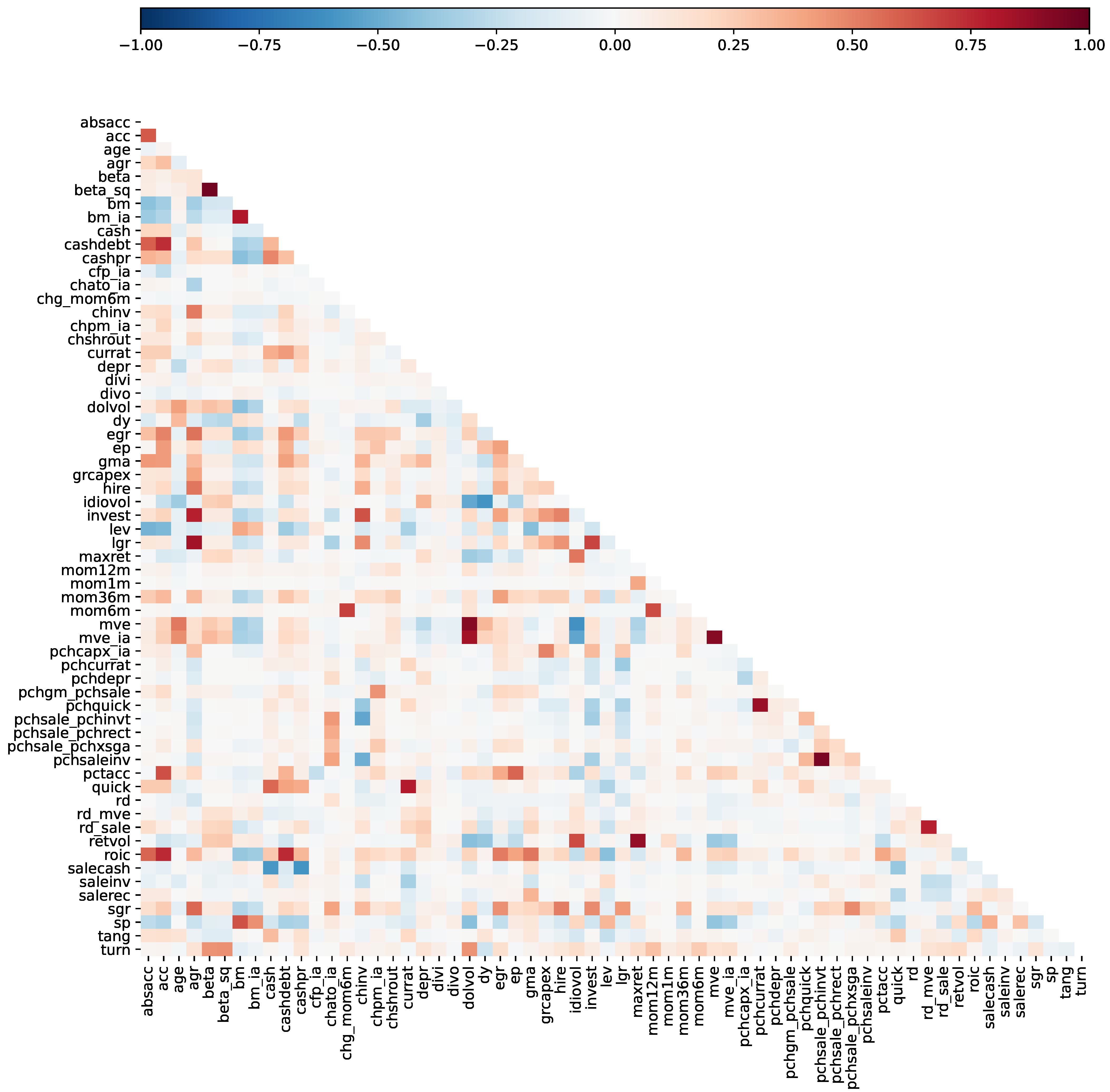
This study contributes to the literature by developing an extensive Monte Carlo simulation to generate a panel of plausible cross-sectional returns in which a distinct and novel feature is the flexible simulation of high-dimensional FC correlation matrices. This simulation design allows us to investigate extensively the predictive performance of Lasso methods in panels for various error specifications and to highlight eventual problems related to the correct selection of FC that contain useful information to predict the cross-section of expected returns.
The primary goal of the paper is to answer the question of whether Lasso-type methods can be useful in predicting differences in expected cross-sectional returns. Secondly, the paper aims to determine which firm characteristics drive these predictions and how they compare to classical approaches. In addition to the empirical evaluation, we use a simulation study to shed light on the properties of the methods in finite samples. For the empirical part of our analysis, we focus on the US cross-section. We include 62 published firm characteristics constructed based on the CRSP/Compustat merged database with monthly data starting from 1974 until 2020.
It is important to note that we constrain our selection and prediction procedure to the linear setting. Specifically, we want to perform our prediction based on a multivariate regression that is consistent with the original scope when the considered FC was introduced in the literature. Hence, this study builds on the work of Green et al. [
3]. In particular, the authors analyze a large set of FC in a linear multivariate Fama and MacBeth [
8] regression; we closely follow their data construction and FC pre-selection procedure. However, instead of relying on a multivariate regression, we apply the adaptive Lasso a true variable selection method.
The simulation results indicate some advantages of the adaptive Lasso over the Lasso in selecting the true set of FC. In contrast, Lasso-type predictions rank consistently better when predictive accuracy is the main objective. We find patterns consistent with the simulation results when predicting US small-cap stock returns, as two of the considered Lasso-type specifications achieve the best predictions. Large-cap stocks are not forecastable with the methods included in this work and the naïve zero return forecast cannot be rejected as being inferior to the included set of linear estimators. These results on the US expected returns cross-section confirm and extend the empirical evidence provided in the previous literature.
The full pooled panel adaptive Lasso selection characterizes 21 FC of relevance for future differences in stock returns. This is in stark contrast to 47 variables selected by the Lasso, 23 by pooled ordinary least squares (POLS) and 13 by POLS inference corrected for multiple testing. The most dominant FC for prediction is based on price information; the most consistently selected is short-term reversal. Moreover, the Fama and French [
9] five-factor model is fully represented in the Lasso-based selection, but complemented by additional FC. Although the methods considered in the current study substantially differ, generally this contrasts with the findings of Green et al. [
3], as they identify a relatively low-dimensional linear cross-section.
This study contributes to different strands of the literature. First, it contributes to the asset pricing literature by analyzing the usefulness of Lasso-type methods in selecting relevant FC for estimating and predicting expected cross-sectional stock returns; we refer, among others, to Cochrane [
10,
11], Goyal [
12], and Hou et al. [
13] for reviews of the different research questions, estimation methods, and introduced FC related to asset pricing. Harvey et al. [
1] introduce the concepts of family-wise error and the false discovery rate to the finance literature. Applying the t-value adjustment reveals that many published factors would lose their status as a significant factor. However, the method suffers shortcomings from a prediction perspective that our work takes into consideration: It does not explicitly take into account the dependence structure of the FC and it neglects to trade-off type I vs. type II errors.
More recently, Kozak et al. [
14] investigate the problem from a portfolio perspective in combination with
and
penalties. The authors identify a sparse set of FC. A mean-variance (MV) optimized portfolio including 50 anomaly variables yields a CAPM alpha similar to the Fama and French [
9] five-factor model. Furthermore, the authors include two-dimensional interactions between these 50 FC and show a substantial increase in an alpha of the MV portfolio compared to the case without interactions.
Feng et al. [
15] propose a double Lasso model selection methodology to systematically investigate the in-sample marginal contribution to asset pricing of some new, additional factors beyond what is explained by a possibly vast number of already existing ones. They introduce a framework for conducting in-sample statistical inference in such a high-dimensional setting and provide robustness checks to verify the sensitivity of the results with respect to the involved tuning parameters in finite samples. In contrast to their study, our analysis focuses on out-of-sample prediction and on the evaluation of the forecasting accuracy of the resulting Lasso-based models. We provide new evidence about the finite sample properties of the Lasso (and other) estimators to select relevant factors for prediction through an extensive simulation exercise that is broader in terms of competing models and model selection criteria designed for forecasting than the one presented by Feng et al. [
15].
Finally, Bryzgalova [
16] pays particular attention to problems arising from model misspecification when using shrinkage methods in the context of factor models. She introduces an alternative adaptive weighting scheme based on partial correlations instead of a two-stage procedure as compared with the adaptive Lasso. The work of Freyberger et al. [
17] approaches the problem using non-parametric techniques. DeMiguel et al. [
18] analyze the FC selection from a portfolio perspective in a framework that combines shrinkage and mean-variance (MV) optimization. Moreover, a fast-growing strand of the literature addresses the prediction problem from a non-linear perspective; see, for example, Messmer [
19], Moritz and Zimmermann [
20] or Gu et al. [
21].
Second, our study is related to the literature that investigates the finite samples or asymptotical properties of shrinkage approaches in financial settings. The Lasso introduced by Tibshirani [
6] is motivated by the desire to improve OLS estimates without the shortcomings of subset selection and ridge regression. Tibshirani [
6] notes that subset selection suffers from high variability, as small data changes can cause subset selection to easily select a different model. Zou [
7] remarks that subset selection can become computationally infeasible if the number of variables is large. Ridge regression, which penalizes the sum of the squared coefficients (
norm) in a linear regression framework, on the other hand, has no obvious interpretation due to the fact that the coefficients are not exactly set to zero.The Lasso estimator optimizes least squares under an additional condition involving the total sum of the absolute size of the coefficients (known as the
-norm) that cannot be larger than a given tolerance value. The inclusion of a penalty term leads to consistent coefficient estimation and variable selection if two necessary conditions are fulfilled, as Meinshausen [
22] shows; see Bühlmann and Van De Geer [
23] for a detailed discussion. These conditions are too restrictive in many empirical applications. Zou [
7] modifies the Lasso insofar as the weight of each coefficient in the penalization term is adaptive. This is achieved by scaling the absolute value of each coefficient with a first-stage estimator such that more highly relevant variables are less strongly affected by the penalty. Setting adaptive weights leads to consistent variable selection and coefficient estimation even if one of the two is not fulfilled.
The previously mentioned consistency properties are developed for a cross-sectional set-up with iid errors. Typically, the majority of applications in finance require the use of time-series or panel data. Moreover, an iid error specification is more an exception than the rule. Consequently, Medeiros and Mendes [
24], Caner and Zhang [
25], Caner and Kock [
26], Kock and Callot [
27], Audrino and Camponovo [
28] and Kock [
29,
30] derive asymptotic properties of the Lasso and the adaptive Lasso in time series and panel settings. In particular, Medeiros and Mendes [
24] and Audrino and Camponovo [
28] derive consistency properties of the adaptive Lasso in time series environments. Medeiros and Mendes [
31] prove that the oracle properties of the adaptive Lasso are preserved for linear time series models even under non-Gaussian, conditionally heteroscedastic and time-dependent errors. Audrino and Camponovo [
28] show that the adaptive Lasso combines efficient parameter estimation, variable selection and valid finite sample inference for general time series regression models. We contribute to this strand of the literature by investigating the finite sample properties of Lasso-type estimators by performing extended simulations in a realistic panel data setting mimicking closely the behavior of the expected returns cross-section with a prediction target.
The paper is organized as follows.
Section 2 provides a description of the relevant methodology. This section is followed by a description of the estimation objective and how it relates to a factor structure.
Section 3 presents the simulation study. The data are briefly discussed in
Section 4. The penultimate section covers the empirical work, including the return prediction and FC selection results. The final section concludes.
2. Methodology
This section introduces the notation and presents the underlying estimation methods and the statistics we use to evaluate the selection and prediction performance of the methods in our simulations and the empirical analysis.
2.1. Notation
Generally, if not explicitly otherwise stated, we follow the notation that
n refers to stock
n of
total stocks and
t to period (i.e., month)
t of
T total periods. Moreover, factors are indexed by
c of
C total factors and belong to set
, where each
c belongs to one of the following three groups or subsets: priced factors are denoted by
p (of a total
P) and define the set
; unpriced factors are defined by
u (of a total
U, set
), and spurious factors with respect to the return process are described by
s (of a total
S, set
). The total number of factors,
. A specification of each type of factor is outlined in more detail in
Section 2.2. The indexing of FC is identical to that of the factors.
2.2. FC and the Return Generating Process
Generally, we assume a Rosenberg [
32] and Daniel and Titman [
33] type cross-sectional return structure. Covariances are determined based on a factor structure and expected returns mark a compensation for factor risk (default assumption). Following Daniel and Titman [
33], we consider the following excess return generating process,
where
defines the vector of factor returns of length
C and
each stock idiosyncratic noise component, assumed to be normally distributed and orthogonal to the factors and other stocks’ idiosyncratic components.
, the vector of the corresponding
C FC and an intercept:
. Each factor,
, follows the dynamics,
where
defines the risk-premium of the
i’th factor and
the sequence of independent factors’ innovations. Moreover, we assume a linear functional relation of the FC and the factor exposures,
with
B a
matrix of coefficients. Note that
cancels, once we consider de-meaned cross-sectional returns. Naturally, exposures are time-varying. This is in line with the empirical characteristics, as momentum or value exposures vary with the price level movements of each stock. The model
1 then becomes
where
is the new zero mean innovation. As a consequence, the linear predictive dependence we aim to measure is of the form:
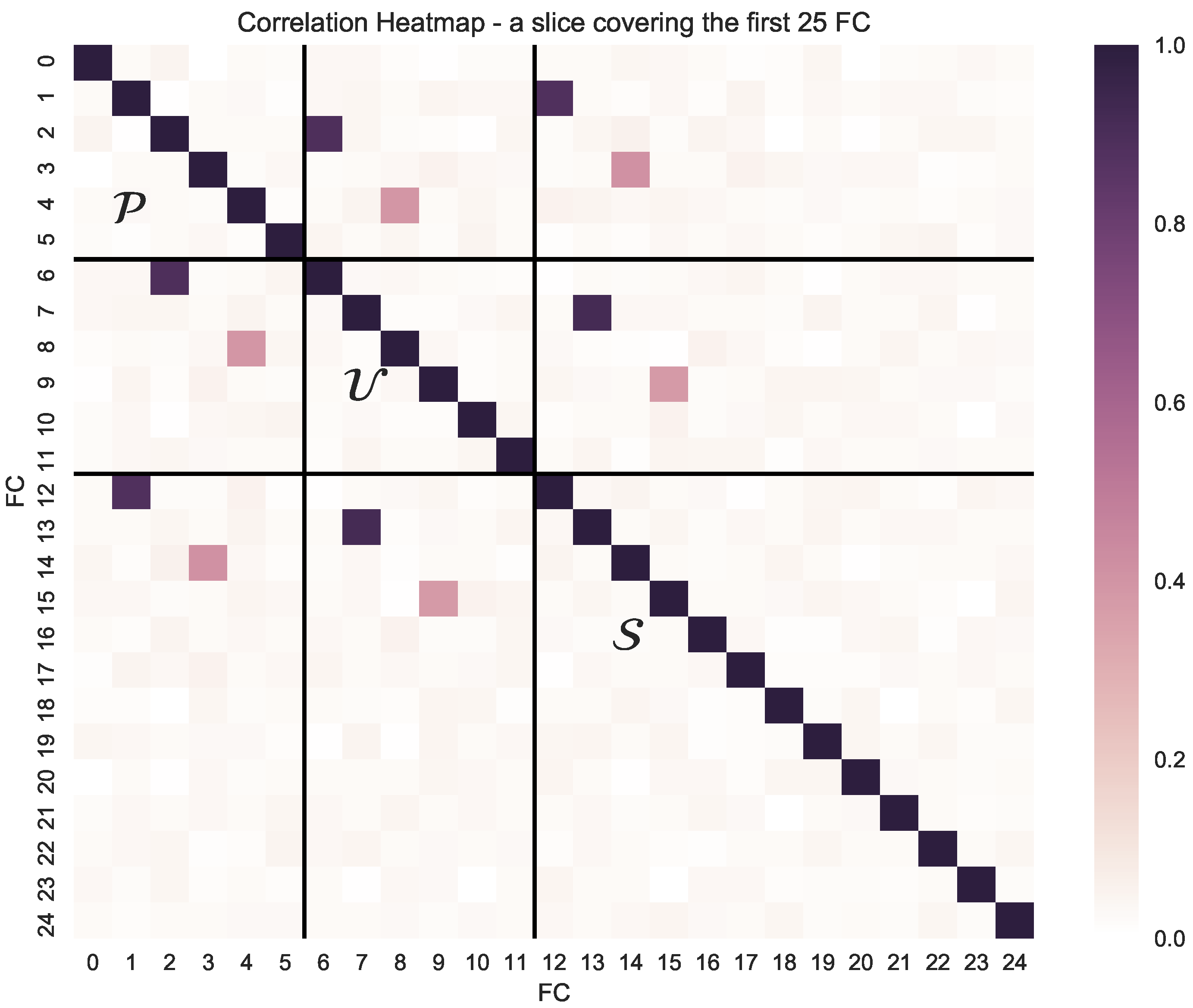
To allow for different interpretations of the relationship between FC and expected returns from an asset pricing perspective we differentiate among three types of factors, namely priced, unpriced, and spurious factors:
P priced factors: ,
U unpriced factors: ,
S spurious factors: .
Examples of priced factors are the market or value factor; for unpriced factors, sector factors; and for spurious factors, an independently created random time series. In a first model setting we consider risk-premia always coupled to the underlying risk-exposure, that is and , where denotes the column of B. As an example, the CAPM can be found in this asset pricing model interpretation by considering only one priced factor, the market factor and no unpriced or spurious factors.
Under a second asset pricing modeling interpretation, we consider a model where
is not constrained to be equal to zero for the unpriced factors in (
3). In case
for some
,
measures the sensitivity of FC to expected returns that do not directly compensate for factor risk. It imposes a non-zero covariance between FC (
) and some factors in case the FC are linked to the non-zero elements in
as described in Daniel and Titman [
33]. In this model setting, we might have zero-priced factors. In particular, this asset pricing model allows two stocks with an identical book-to-market ratio to have different risk exposures to a book-to-market value factor. Here the return compensation is associated with the book-to-market characteristic, i.e., mispricing, and not its risk sensitivity to the value dimension. The first asset pricing modeling framework rules this out. The second asset pricing model implies the presence of asymptotic arbitrage. Regardless of the interpretation, both models are estimated using (
3).
2.3. Methods
We focus on three different linear models, which are defined as:
where
and
and the corresponding response vector
, the design matrix
, the parameter vector
. We slightly deviate in this subsection and denote the regression coefficient as
(vs.
). In all other sections we use the term
exclusively as a measure of factor exposure, and
as the regression coefficient we aim to estimate. Moreover, throughout this work we treat
and
as standardized matrices, with
and
, where the standardization is applied column by column. As defined in (
1)
corresponds to the vector of excess returns,
, and
to the matrix of FC. Equation (
4) defines the ordinary least squares (OLS) estimator, Equation (
5) the Lasso estimator (Tibshirani [
6]) and (
6) the adaptive Lasso (Zou [
7]). The Lasso and the adaptive Lasso differ in terms of the penalization term, which allows the weights to vary for each parameter. The assigned individual weights are inversely proportional to a first-stage
estimate. Zou [
7] suggests the use of the OLS estimator,
as
, unless collinearity is an issue. Bühlmann and Van De Geer [
23] set
. The use of the Lasso as a first-stage estimator is justified by the screening property of the Lasso, which still allows consistent variable selection of the adaptive Lasso at the second stage. We solely use the Lasso as a first stage estimator in (
6) in this work. The penalty term
used in (
5) and (
6) is determined by cross-validation (CV) or classical selection criteria, typically five-fold or ten-fold CV, the Bayesian information criterion (BIC), or the Akaike information criterion (AIC). Bühlmann and Van De Geer [
23] show that the optimal
based on the BIC evaluation reads as follows:
and accordingly the AIC,
Alternatively, the optimal can be estimated by cross-validation. Here we randomly split the samples along time points and never within a given period. Assume we observe T periods each containing N stocks , ,..., . Consequently, we can randomly select a training and testing set along the time index t. Hence, high cross-sectional correlations cannot cause biased estimates for the optimal .
The empirical set-up presented above makes shrinkage methods like the ones introduced above an attractive choice as they possess the ability to reduce the variance at the cost of slightly increasing the bias. First, as the variance increases in p, the ratio of can potentially be high, as we have 400+ presented factors in the literature and in the best case 50 years of monthly data (). Moreover, if some FC is available only for a shorter period of time, we can still perform the regression, as the Lasso methods are feasible even for the case where we have a truly high-dimensional problem (), which imposes a constraint for classical OLS. Moreover, the noise component makes up unambiguously a significant proportion of the return process (even when assuming that the efficient market hypothesis is violated). Hence, the noise variance component has an important impact.
2.4. Data Sparsity
It is important to highlight the role played by the assumption of data sparsity connected to the use of the (adaptive) Lasso. Data sparsity is generally an untestable assumption and we consider it only a rough although reasonable approximation of reality. According to Zhang et al. [
34] the concept of exact sparsity can be relaxed while still maintaining the same rate of convergence of the Lasso estimator to the true coefficients. They define that a model is sparse if most coefficients are small, in the sense that the sum of their absolute values is below a certain level. Under this general sparsity assumption, it is no longer sensible to select exactly the set of nonzero coefficients. Therefore, in cases where the exact selection consistency is unattainable or undesirable, the authors show that the Lasso is able to select the important variables with coefficients above a certain threshold determined by the controlled bias of the selected model. Thus, under this generalized sparsity concept, the (adaptive) Lasso is able to successfully discriminate between small and large coefficients and identify with high probability the most important firm characteristics; see also Bühlmann and Van De Geer [
23] for a general review of the corresponding theory.
Moreover, given that our interest focuses primarily on the predictive ability of the competing approaches, the results discussed by Greenshtein et al. [
35], Bickel et al. [
36], and Sirimongkolkasem and Drikvandi [
37] are reassuring: They highlight the fact that assuming sparsity as an approximation of the true design of the data does not generally significantly degrade the predictive accuracy of the models in high-dimensional settings with a large number of covariates. Greenshtein et al. [
35] show that under various sparsity assumptions there is “asymptotically no harm” in considering a large number of covariates (many more than observations) for prediction purposes in a linear regression model under an
constrained optimization. Bickel et al. [
36] provide bounds on the
prediction loss,
, of the Lasso in a high dimensional linear regression in terms of the best possible (oracle) approximation under the sparsity constraint. Finally, by comparing different shrinkage approaches in a linear regression simulation setting, Sirimongkolkasem and Drikvandi [
37] show that when important covariates are associated with correlated data, the
and
prediction performances of the Lasso improve for both sparse and non-sparse high dimensional settings and even sometimes outperform those of the Ridge regression. The predictive performance of the Lasso remains generally unaffected when the correlated covariates are associated with nuisance and less important variables. Given the previous evidence and the fact that the focus of the current study is set on identifying the most relevant methods and firm characteristics for predicting the cross-section of expected returns in a variable selection framework, we do not report results for alternative shrinkage techniques like the Ridge. Predictive performance results using Ridge are qualitatively similar to those presented for the lasso in
Section 5.2.1 and are available from the authors upon request.
2.5. Selection and Prediction Evaluation
We apply pooled ordinary least squares as described in (
4), where the t-values are based on the Driscoll and Kraay [
38] robust standard errors. Next, we set a significance level for the OLS estimates to have a rule determining whether or not a coefficient can be seen as selected—we set the level to the literature standard of 5%. The impact of multiple-testing is gauged by considering t-value corrections as presented by Harvey et al. [
1]. Specifically, we use the Bonferroni and Holm adjustment, which belongs to the class of family-wise error rates. Additionally, the study includes Benjamini, Hochberg and Yekutiel’s (BHY) adjustment, a false discovery rate control, which we also consider; we refer to Harvey et al. [
1] for a more complete description of the multiple-testing adjustments. In the case of the Lasso and the adaptive Lasso, the FC selection procedure is straightforward: all non-zero coefficient estimates are considered to be selected. Here we provide estimates for Lasso- and adaptive Lasso-based BIC, AIC and five-fold cross-validation (CV5) optimized regularization strength.
Following the variable selection, we calculate expected returns for each stock at each point in time. In this step, we evaluate two variants of each method. The first case drops all insignificant coefficients in the case of OLS and takes the relevant ones directly into consideration for the prediction. The second variant performs a post-variable selection OLS (PVSOLS).
The prediction quality is then measured based on a cross-sectional average, as proposed by Gu et al. [
21]. More formally,
where
and
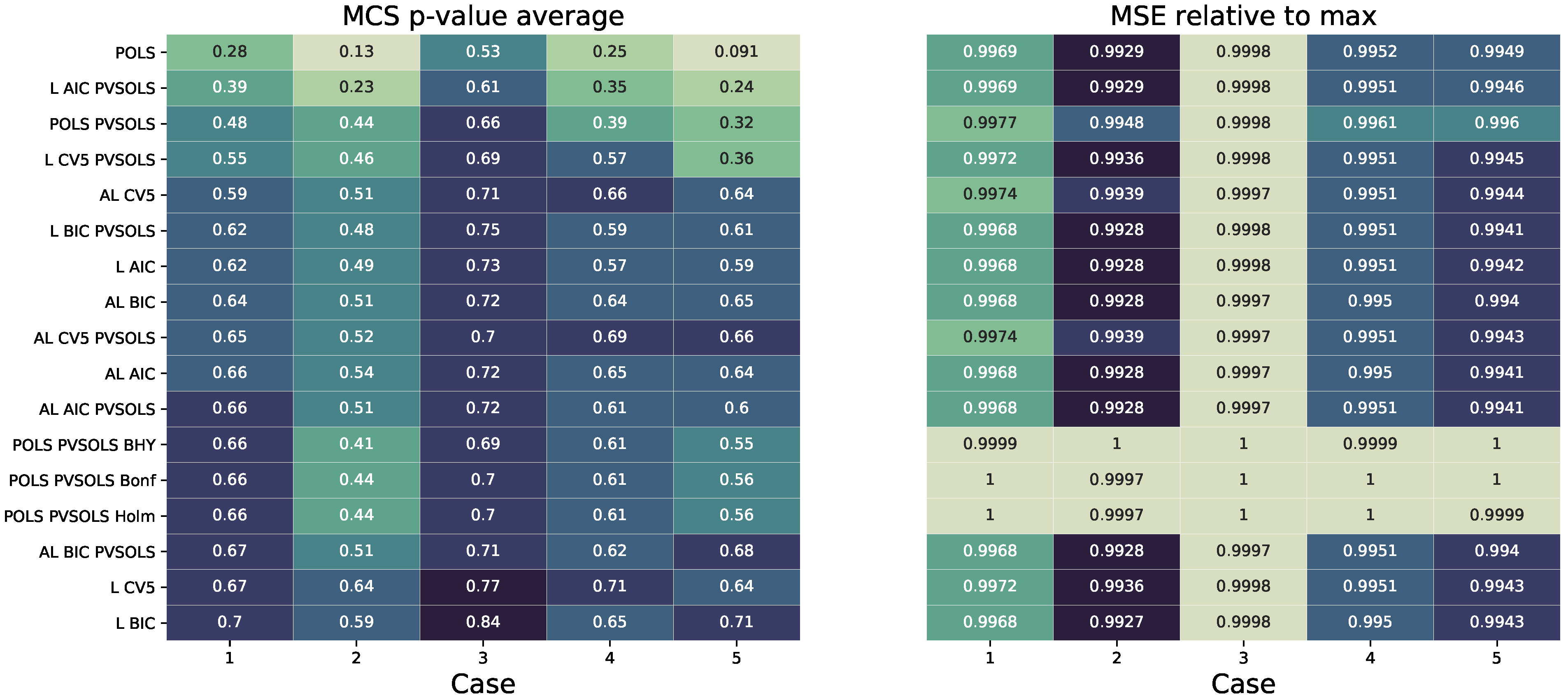
denote the actual and the predicted excess returns over the risk-free rate, respectively. We report two metrics measuring the prediction performance, the simple time series average of
and the model confidence set (MCS) as introduced by Hansen et al. [
39].
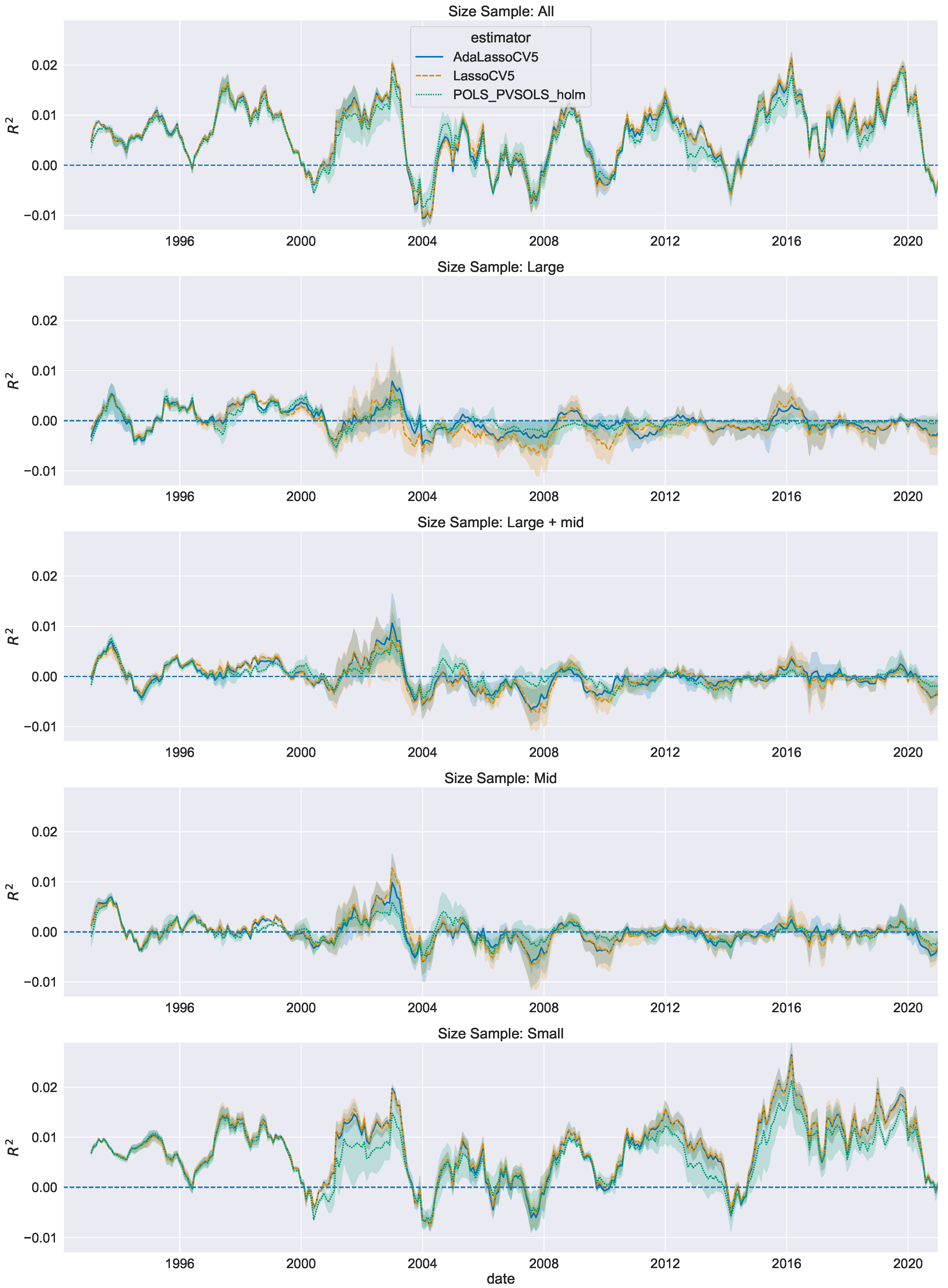
Furthermore, we report the out-of-sample
following Campbell and Thompson [
40] defined as follows:
4. Data
Our objective is to preserve consistency as much as possible. Therefore the selection, data preparation and the notation of the description of firm characteristics generally follow the approach of Green et al. [
3]. The FC data are implemented independently of Green et al. [
3]. Our sample period ranges from 1974 to 2020. As in most studies, the analysis considers only CRSP stocks with share codes 10 and 11 which are traded either at NYSE, AMEX or NASDAQ; for an example, see Fama and French [
4]. Furthermore, we exclude stocks with missing market capitalization data and/or where book values are unavailable. Compustat data are aligned with a standard lag of six months of the fiscal year end date. For example, the data of a firm with fiscal year end date 12/31 are aligned with data 06/30, predicting monthly returns from 6/30 to 7/31. CRSP-based stock/firm characteristics, such as idiosyncratic volatility, beta, maximum return or six-months momentum are used as of the most recent month end. For example, for the return prediction from 6/30 to 7/31, the max daily return from the period 5/31-6/30 is used. Additionally, following Green et al. [
3] some selected Compustat accounting data are set to zero if not available; see the
Appendix A for details. In processing larger amounts of data, correcting extreme and often implausible values is mostly unavoidable. Correcting these values on a discretionary basis is not feasible; hence, winsorizing the data is a useful strategy to reduce the problem. Therefore, each FC is winsorized at the 1% and 99% percentile at each point in time. Binary FC like
divi,
divo,
rd and
ipo are excluded from the winsorizing procedure. In the next step, missing data are replaced by the mean of the winsorized data at each point in time. Only then can the z-score standardization be applied at each calendar point. We do winsorize the return observations at the 5% and 95% percentile at each point to reduce the weight of outliers in the least-squares setting; therefore, no observations are excluded because of implausible returns. Moreover, returns are only de-meaned for each period and not corrected by the standard deviations. Finally, the data can be stacked and the pooled regressions applied, as each independent variable has mean zero and variance one given by the property of combining z-scores. Note that this is necessary as the Lasso requires a normalized design matrix as input, as described above.
However, differences in the selection of FC are unavoidable. This study employs only FCs which are not dependent on Compustat quarterly and IBES data. A detailed description of each FC included in the empirical part of this study can be found in the
Appendix A. Moreover, the
estimates are obtained by regressing rolling weekly stock returns on the market excess returns. The literature often employs an alternative procedure whereby stocks are ranked and sorted into portfolios according to their individual market beta; see, for example, Fama and French [
4]. The betas assigned to each stock for estimating the equity market premia are obtained by using the betas of the corresponding portfolios. Using portfolio beta estimates instead of individual stock betas has been applied to reduce potential errors-in-variable issues in the second stage regression. However, Ang et al. [
45] cast doubt on whether portfolio betas are optimal due to the loss of dispersion in individual betas. More details about the specific CRSP and Compustat data and the corresponding data alignment process can be found in the
Appendix A. The returns used in the prediction regression are the CRSP returns (
RET) adjusted by the provided CRSP delisting return (
DLRET). Additionally and for verification purposes, we benchmark our data for selected FC with the FC portfolio returns provided by Kenneth French’s Data Library. We find satisfying
s, reaching values from
to about 0.9 for cases where the FC definition of the benchmark data slightly deviates from the one presented in Green et al. [
3]. Furthermore, we follow Fama and French [
46] for the size classification definition, where large-cap stocks are the 1000 stocks with the highest market capitalization, mid-cap stocks rank 1001–2000 and small comprise all stocks with rank
. Finally, our industry-adjusted variables always use the 48 sectors downloaded from Kenneth French’s Data Library, as the SIC 2 classification is empirically too granular since in many instances the sector group is defined by a single stock.


