Article

Four-Parameter Weibull Distribution with Lower and Upper Limits Applicable in Reliability Studies and Materials Testing

Department of Mathematics and Physics, Military Technology Faculty, University of Defence, Kounicova 65, CZ-662 10 Brno, Czech Republic
Mathematics 2023, 11(3), 544; https://doi.org/10.3390/math11030544
Submission received: 13 December 2022 / Revised: 13 January 2023 / Accepted: 18 January 2023 / Published: 19 January 2023

Abstract

:
A simply curved Weibull plot means that the studied data set has a three-parameter Weibull distribution with a non-zero location parameter representing the lower or the upper limit of the data set. This paper introduces a four-parameter Weibull distribution with both of these limits that can be applied in both reliability and materials engineering. A very reliable indicator of this distribution is the double-curved Weibull plot. The great advantage of this distribution is the fact that the corresponding hazard rate curve can be bathtub-shaped with a great ability to fit the measured data.

1. Introduction

The Weibull plot with the concave shape of an empirical curve mostly indicates the necessity to use the three-parameter Weibull distribution with a nonzero location parameter, which represents the lower limit of a studied data set. Similarly, a three-parameter Weibull distribution function with the localization parameter representing the upper limit of the studied data set was recently proposed, and several examples of applying this distribution to convexly curved Weibull plots were presented. This paper proposes a four-parameter Weibull distribution function with both the lower and the upper limits of the studied data set suitable for the twice-curved Weibull plots. Some examples of applying the newly proposed function are presented: for lifetime or time-to-breakdown in reliability studies and for strength properties in material testing.
The distribution with the cumulative distribution function (CDF)
P ( t ) = 1 exp [ ( t η ) β ] for t 0 P ( t ) = 0 for t < 0
is called the (two-parameter) Weibull distribution [1], where t is a variable (e.g., time to breakdown, strength, etc.), η is the scale parameter, and β is the shape parameter. In the lnt vs. ln{ln[1/(1 − P)]} or lnt vs. ln[−ln(1 − P)] plot called the Weibull plot; the CDF is plotted as a straight line with the slope β because Equation (W2) can be rewritten in the linear form
ln ln 1 1 P ( t ) = β ln t β ln η .
In the Weibull plot, the scale parameter η corresponds to such t* value, for which the equality ln{−ln[1 − P(t*)]} = 0 applies, i.e., for 0 value on the vertical axis on the Weibull plot.
For the set of the measured values t1, …, tn the Weibull plot can be drawn, where the determination of the Pi values of cumulative probability is necessary. It is usually based on the relative cumulative frequency φ. For ordered ti values t1 < t2 < … < tn the φ function has jump discontinuities
φ ( t i ) = i 1 n   and   φ + ( t i ) = i n .
Conventionally their mean is considered for the Pi values
P i = i 0.5 n .
Moreover, very often, the Weibull approximation [2]
P i = i n + 1
and the Benard approximation [3]
P i = i 0.3 n + 0.4
are used. General equation is
P i = i a n + 1 2 a
where a is equal to 0 (Weibull), 0.3 (Benard), 0.333 (1/3), 0.375 (3/8) or 0.5 (1/2, conventional value).
In most cases, the Weibull plot does not have a simple linear course but a more complicated shape. Then, the piece-wise linear dependence is sometimes assumed because of varying mechanisms of the studied phenomena. In the case of a smooth concave shape of the empirical Weibull plot with the left end tending towards the lnt0 value on the lower lnt axis, the three-parameter Weibull distribution
P ( t ) = 1 exp [ ( t t 0 η ) β ] for t t 0 P ( t ) = 0 for t < t 0
can be considered, where t0 is the location parameter. If t means time, t0 is referred to as failure-free time or minimum lifetime while in the case of mechanical properties, t0 is called the threshold or the minimum value of studied property.
For the description of a smooth convex shape of the empirical Weibull plot with the right end tending towards the lnt value on the upper lnt axis, the three-parameter Weibull distribution
P ( t ) = 1 exp [ ( 1 η t t t t ) β ] for 0 t < t P ( t ) = 0 for t < 0 P ( t ) = 1 for t   t
was derived, and several successful applications in reliability studies, as well as in material testing, were presented [4]. The parameter t is, in fact, also a localization parameter, and it could be called maximum lifetime, maximum strength, etc., depending on which quantity was measured.
The shape of some empirical Weibull plots is more complicated: their left part is concave with the end tending towards the lnt0 value on the lower lnt axis, while their right part is convex with the end tending towards the lnt value on the upper lnt axis. In such cases, three lines are often used for the fit (see, e.g., [5], specifically, Figure 9 in [5]), although the course of the empirical dependences is very smooth, without a slope discontinuity. Another possibility is a combination of Equations (W3min) and (W3max) leading to a four-parameter Weibull distribution. The transition from Equation (W2) to Equation (W3min) consists in replacing the expression t with the expression tt0. Similarly, a relation for a four-parameter Weibull distribution can be obtained based on Equation (W3max) applying the same replacement ttt0. There are two ways how to do this. The first way is
t t t t t ( t t 0 ) t ( t t 0 ) = t t t 0 ( t + t 0 ) t t t t 0 t t
where in the denominator t0 is neglected relative to t. The second way is
t t t t t t t t t 0 = ( t + t 0 ) t t t 0 t t t t t 0 t t
where t0 is neglected relative to t in the numerator. Both ways lead to the same result,
P ( t ) = 1 exp [ ( t η t t 0 t t ) β ] for t 0 t < t P ( t ) = 0 for t < t 0 P ( t ) = 1 for t   t
which represents the four-parameter Weibull distribution with the lower limit t0 and the upper limit t. However, it is necessary to keep in mind the condition used in the derivation (see Equations (7) and (8)), which is also the condition of validity of Equation (W4): t0 << t. This means that the lower limit of the distribution should be at least an order of magnitude smaller than the upper limit. Fortunately, this condition can be attenuated in Equation (W4) for certain values of the exponent β. The correctness of the above derivation can be verified by reverse simplifications
t t t 0 t t t t 0 for t < < t t t t 0 t t t t t t for t > > t 0
i.e., Equation (W4) → (W3min) for t << t and Equation (W4) → (W3max) for t >> t0.
The probability density function (pdf) corresponding to the (W4) CDF can be simply obtained by the differentiation of the CDF
p ( t ) = β η exp [ ( t η t t 0 t t ) β ] ( t η t t 0 t t ) β 1 t ( t t 0 ) ( t t ) 2 for t 0 t < t p ( t ) = 0 for t < t 0 and t   t .
Already in 1958, Kies published a modified Weibull CDF with both the lower and the upper limits of the studied data set suitable for the twice-curved Weibull plots [6]
P ( t ) = 1 exp [ α ( t t 0 t t ) β ]
containing 4 parameters α, β, t0, and t∞, and in 1987, Phani published his modification [7]
P ( t ) = 1 exp [ α ( t t 0 ) β 1 ( t t ) β 2 ]
containing five parameters α, β1, β2, t0, and t (for β1 = β2 = β both modifications are identical). However, both of these CDFs have two beauty defects:
  • If t represents time measured, for example, in seconds, then, the physical unit of the α parameter is sβ in the Kies modification and s β 2 β 1 in the Phani modification (for fracture toughness measured in MPa m0.5, the unit is even more complicated). The parameters with such dubious units cannot have any meaningful interpretation. In the (W4) CDF, all quantities have the same unit (s, MPa m0.5, etc.).
  • The simplification for t0 << t << t leads to
P ( t ) = 1 exp [ α ( t t ) β ]
for the Kies modification and to
P ( t ) = 1 exp [ α t β 1 t β 2 ]
for the Phani modification while the same simplification of the (W4) CDF leads directly to the (W2) CDF.
Both these beauty defects show that the (W4) CDF is more appropriate than the Kies modification. The CDFs with more parameters than four will be discussed below. On the other hand, for
α = ( t η ) β
both the Kies modification and the (W4) CDF are fully identical. This means that the (W4) CDF is a more appropriate notation of the Kies modification.
To verify the applicability of Equation (W4), some twice-curved Weibull plots will be presented using this CDF. On the x-axis, the natural logarithm scale (lnt) or the common logarithm scale (logt or t with equidistant labels 10n) will be used in accordance with the papers from which the experimental data were taken for regression calculations. Similarly, the approximation for determining the Pi values will be used in line with the original articles, i.e., corresponding a value in Equation (6) will be chosen. The general description of used calculation methods is given in [4]; some of their specifics will be considered in the Section 6.
When solving most design problems, it is necessary to know either the lower or the upper limit of the property that has been repeatedly determined and whose values form the studied data set. In such cases, either the lower or the upper tail of the distribution is of primary interest, and it is possible to choose from a wide range of classical and modern distributions, which best fit the empirical distribution. In contrast, the goal of this paper is to present the four-parameter Weibull distribution W4 that describes both tails of the empirical distribution while being consistent with all Weibull distributions with a smaller number of parameters, i.e., with W3max, W3min, and W2.
The Phani modification of the Weibull distribution with five parameters can be generalized to a six-parameter distribution, which very successfully fits even twice-curved Weibull plots with a rather complicated course. However, it is questionable whether it has any real practical significance in addition to successful fitting.

2. Examples of W4 CDF Applications in Reliability Studies

For reliability studies, the hazard rate (HR)
h ( t ) = p ( t ) 1 P ( t ) = P ( t ) 1 P ( t )
is very useful. For the (W4) CDF
h ( t ) = β η ( t η t t 0 t t ) β 1 t ( t t 0 ) ( t t ) 2 for t 0 t < t h ( t ) = 0 for t < t 0 and t   t
is obtained. It is bathtub-shaped when
β < β max = t + t 0 t t 0
and for
t min = 1 + β 2 t 0 + 1 β 2 t
it obtains its minimum value
h ( t min ) = 4 β ( 1 β 2 ) ( t t 0 ) ( t η 1 β 1 + β ) β .
Comparison of the (W2), (W3min), (W3max), and (W4) CDFs, shows the following:
  • no bathtub-shaped HR is obtained for the (W2) and (W3min) CDFs,
  • the bathtub-shaped HR is obtained for the (W3max) CDF when β < 1 (see [4]),
  • the bathtub-shaped HR is obtained for the (W4) CDF also when β > 1 (the limit is given by Equation (18)).
This limit depends on the k ratio
β < k + 1 k 1 where k = t t 0
and can be even 3 for k = 2 or 2 for k = 3. For the t0 and t values differing in an order (quite typical case) it is still about 1.2.

2.1. Time-to-Breakdown of Hf-Doped Ta2O5 Capacitors

The time-dependent-dielectric-breakdown characteristics of Hf-doped Ta2O5/SiO2 stack were studied by Atanassova et al. [8]. Figure 1 presents the Weibull plot of the time-to-breakdown of Hf-doped Ta2O5/SiO2 capacitors under stress voltage −4.5 V at temperatures of 20 °C and 80 °C. Because the a parameter from Equation (6) is not listed in the article, the value a = 0.3 has been chosen, i.e., the Benard approximation (5) has been used for the determination of Pi probability values. The fits using Equation (W4) as the regression function give t0 = 78.66 s and t = 36,836 s for the temperature of 20 °C and t0 = 33.75 s and t = 29,204 s for the temperature of 80 °C.
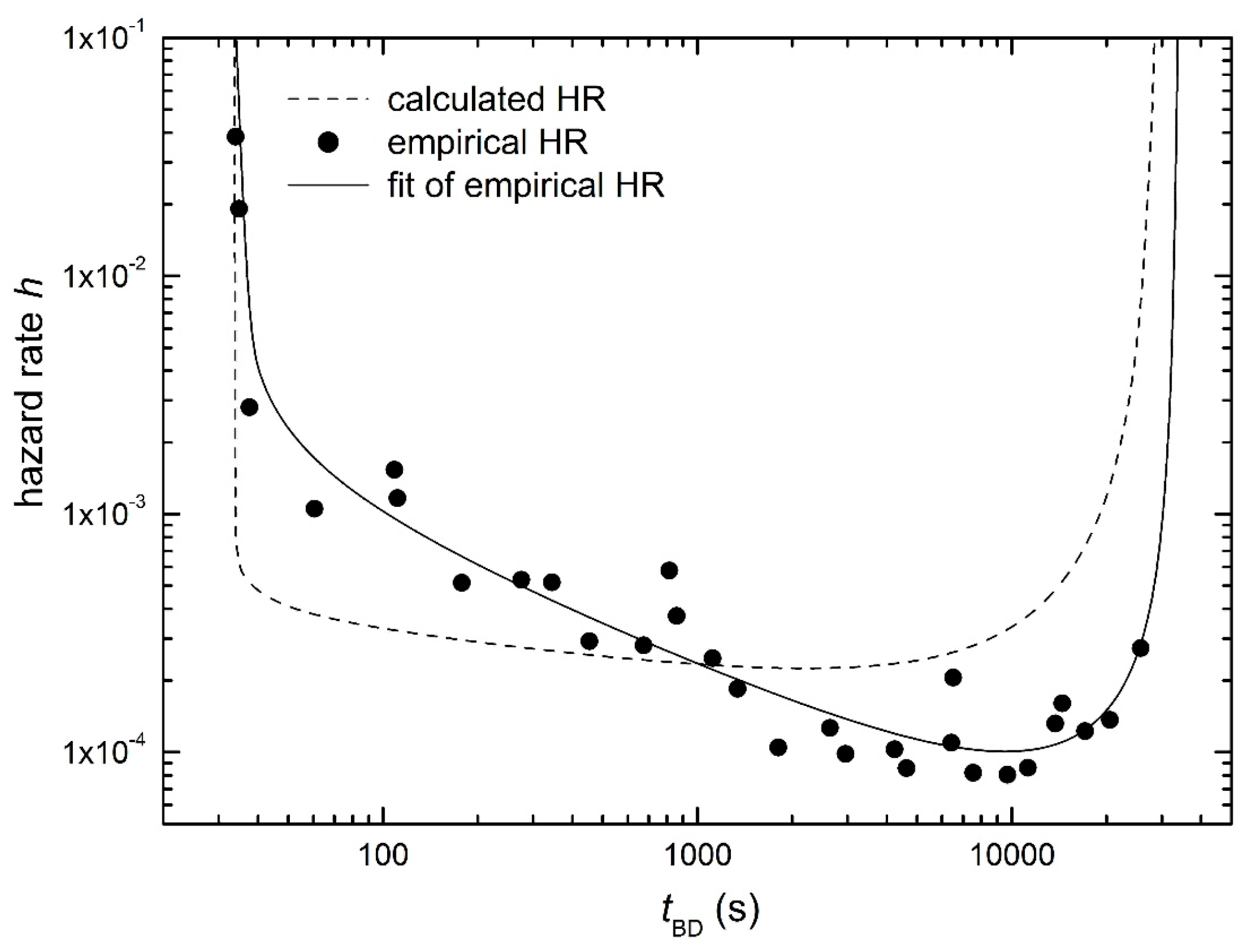
For the presentation of the HR curve, the left curve in Figure 1 (i.e., for the temperature of 80 °C) with a lower dispersion was chosen. The value of the β parameter determined by the LSM (least squares method) of the Weibull plot fitted using the (W4) CDF is 0.849, so the HR curve should be bathtub-shaped. The values of all four parameters of the (W4) CDF determined in this way, substituted into Equation (17), lead to the HR curve represented by the dashed line in Figure 2 (the lin–lin plot) and in Figure 3 (the log–log plot). Moreover, in both figures, the empirical HR is added (see full circles). It was obtained from empirical CDF using relation h(t) = P’(t)/[1 − P(t)] where numerical differentiation of P(t) was used (the first-order two-point formulae were used: right-sided for the first point, left-sided for the last point, and symmetric for the inner points). Finally, the fit of the empirical HR using Equation (17) as the regression function was added (see the solid line in Figure 2 and Figure 3). Since the values of both the time-to-breakdown and HR are over several orders of magnitude, the log–log plot in Figure 3 turns out to be more suitable than the lin–lin plot in Figure 2.
Dissimilar lines in Figure 2 and Figure 3 (dashed lines vs. solid lines) show that the fit of the Weibull plot using the (W4) CDF and the fit of the empirical HR using Equation (17) lead to different values of distribution parameters. As presented in Table 1, all parameters have similar values except for the β parameter, which is almost twice as large in the first case (CDF) as in the second case (empirical HR); also, the values of the t parameter differ by about 15%. The value of the β parameter determines the slope of the middle part of the HR curve in the log–log plot (see Figure 3). In addition to the parameters of the (W4) CDF, Table 1 also contains the positions of the minimum of the HR curves (tmin and h(tmin) values given by Equations (19) and (20), respectively) and the limit values βmax of the β parameter (given by Equation (18)). The different values of the positions of the minimum of the HR curves are mainly the result of the different values of the β and t parameters.
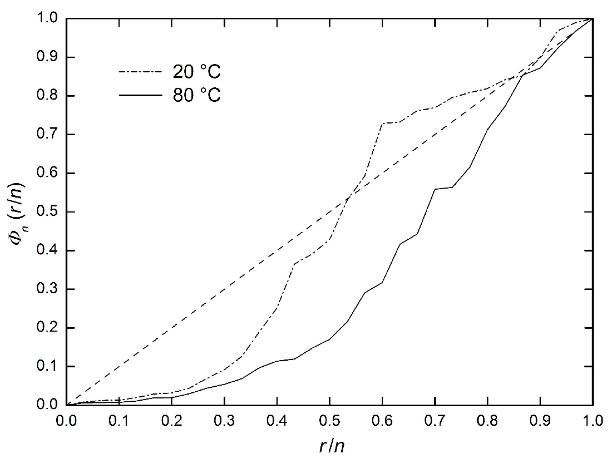
In Figure 2 and Figure 3, both curves, as well as the trend of the empirical points, indicate the bathtub-shaped HR. Nevertheless, a qualitative identification of the trough-shaped HR is added, which does not need any specific form of the CDF or any specific approximation of the empirical values of Pi. It is based on the Total Time on Test (TTT) concept (see Aarset [9]). The TTT plot allows distinguishing among constant, increasing, decreasing, and bathtub-shaped HR, specifically [9]:
  • straight-line plot means constant HR,
  • concavely curved plot means increasing HR,
  • convexly curved plot means decreasing HR,
  • twice-curved S-shaped plot means bathtub-shaped HR.
Let Φn(r/n) is scaled empirical TTT transform given by Equation (22)
Φ n ( r / n ) = [ i = 1 r t i + ( n r ) t r ] / i = 1 n t i
where ti for i = 0, 1,..., n is ordered (from the smallest to the biggest) sample from a life distribution. Then, the TTT plot is the plot of (r/n, Φn(r/n)) for r = 0, 1,..., n, where consecutive points are connected by straight lines. In Figure 4, the TTT plot of the time-to-breakdown of Hf-doped Ta2O5/SiO2 capacitors under stress voltage −4.5 V at two temperatures [8] is presented. The result is quite unexpected—while the plot for the temperature of 80 °C corresponds to the decreasing HR, the plot for the temperature of 20 °C corresponds to the bathtub-shaped HR. Nevertheless, the Weibull plots for both temperatures are qualitatively identical (see Figure 1), and for the temperature of 80 °C, the bathtub-shaped HR was demonstrated in Figure 2 and Figure 3. However, a careful look at Figure 2 and Figure 3 shows that practically only one (the last) point indicates the bathtub-shaped HR, and, on the other hand, the TTT plot (see solid line in Figure 4) shows a certain hint of a twice-curved S-shaped course. Therefore, it is perhaps not surprising that different criteria give different results in this border area.

2.2. Reliability of AlGaN/GaN HEMTS

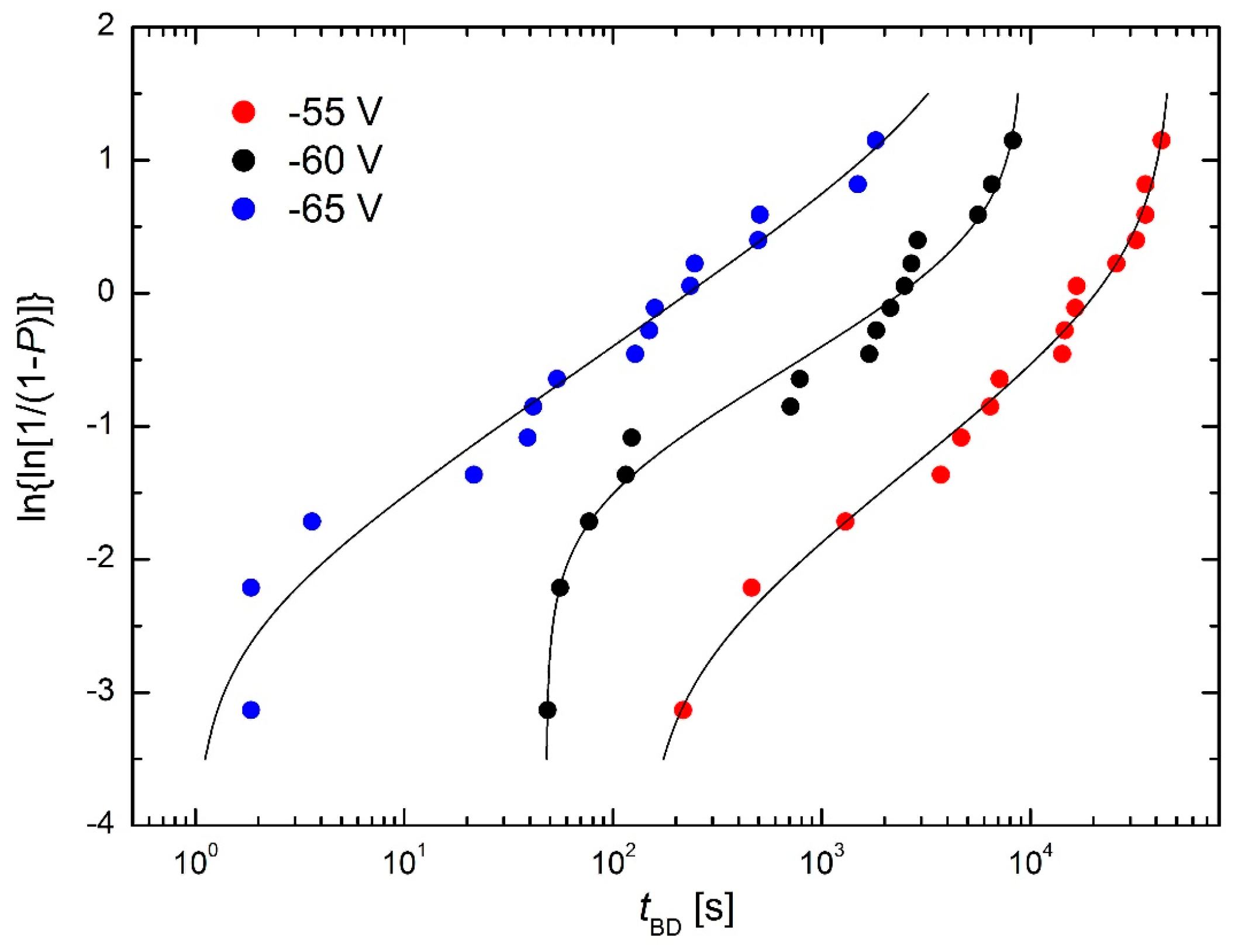
The two most common failure modes of GaN-based HEMTs were studied by Marcon et al. [10]. The time-to-breakdown (tBD) was determined for a wide range of experimental conditions. The Weibull plot of tBD for the temperature of 298 K and three gate voltages of −55 V, −60 V, and −65 V is drawn in Figure 5 (Pi values are determined according to the Benard approximation (5)). The fits using Equation (W4) give t0 = 139 s and t = 48,093 s for the gate voltage of –55 V, t0 = 47.9 s and t = 9115 s for the gate voltage of −60 V, and t0 = 0.983 s and t = 7224 s for the gate voltage of −65 V. All three regression curves show that quite successful fits can be obtained even with a low number of experimental points and their relatively large dispersion.

2.3. Reliability of Multilayer Ceramic Piezoelectric Actuators

The Pb(Mg,Nb)O3-Pb(Zr,Ti)O3 multilayer ceramic piezoelectric devices with dimensions of 5 mm × 5 mm × 5 mm were tested at temperatures from 60 °C to 90 °C and relative humidity of 30% by Koh et al. [11]. Different rectified AC biases were applied to the devices with a fixed frequency of 910 Hz. Reliability tests were carried out until all samples were completely destroyed. The number of voltage cycles to the destruction was taken as a measure of a lifetime. The Benard approximation (5) was explicitly declared for Pi probability values determination (here called a median rank function). The Weibull plot of the number of cycles to destruction for the temperature of 90 °C and humidity of 30 % is presented in Figure 6 for the given rectified AC bias. For the regression, the regression function (W4) is used again, which gives for the AC bias of 300 V the following numbers of cycles: N0 = 1.594 × 10⁷ and N = 2.064 × 10⁹. For the AC bias of 700 V, the regression using (W4) as the regression function was fully unstable, and the fit curve presented in Figure 6 was obtained for firmly given values N0 = 9.79 × 10⁴ cycles (closely below the minimum number of cycles) and N = 1.71 × 10⁸ cycles (closely above the maximum number of cycles). This curve shows that the regression function (W4) is not suitable for the Weibull plot with a very small slope of the middle part (expressed by the value of the shape parameter β ≈ 0.2).

3. Examples of W4 CDF Applications in Material Testing

3.1. Flexural Strength of Aluminum Nitride Ceramics

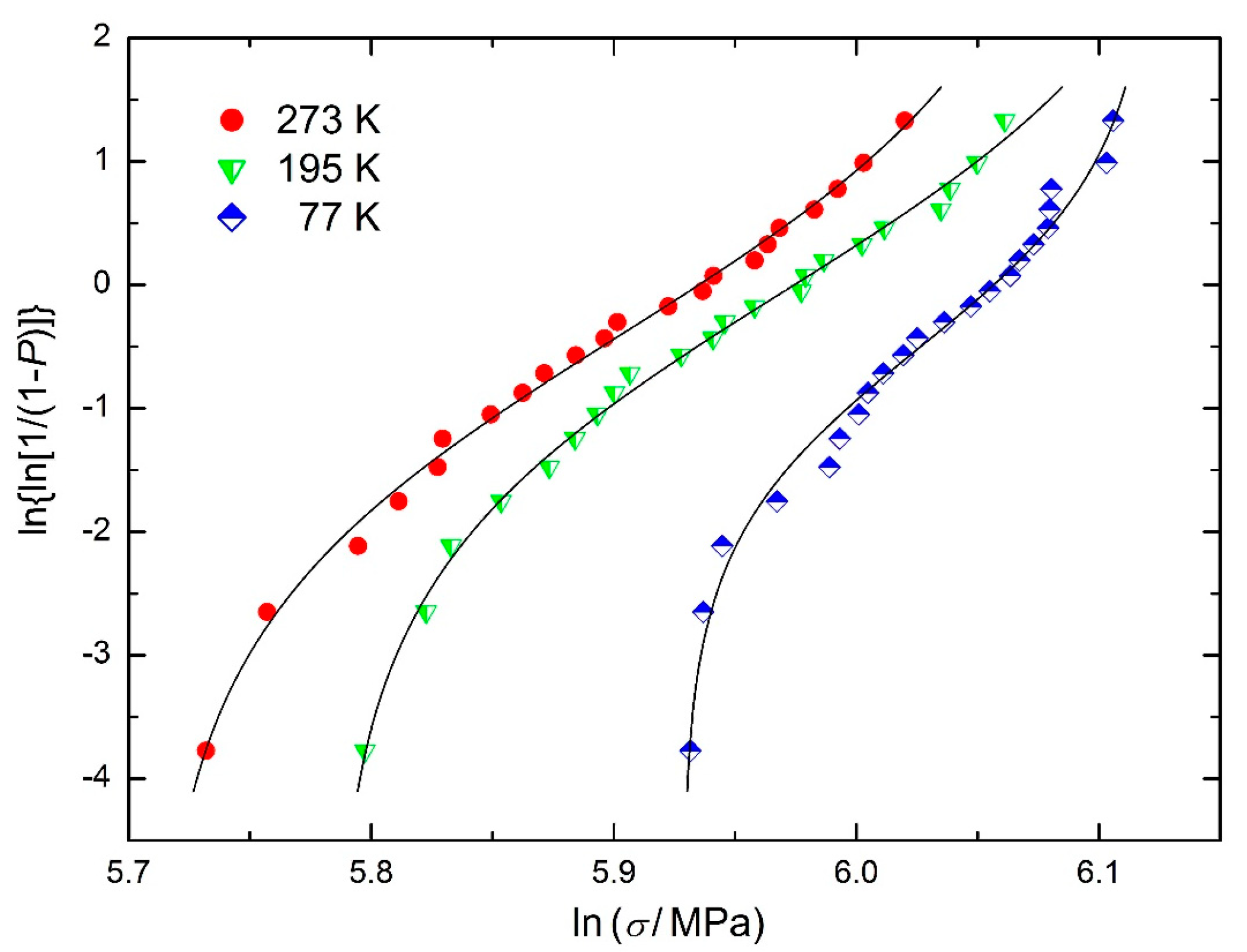
The mixture of raw AlN powder with 5 wt.% Y2O3 powder was pressed (cold isostatic pressing) into blocks and then sintered at 1850 °C for 2 h under an N2 gas pressure of 0.1 MPa by Wei et al. [12]. The blocks, cut with dimensions of 3 mm × 4 mm × 36 mm and polished with diamond pastes, were tested at temperatures of 77 K, 195 K, and 293 K using a three-point bending test. The Weibull plot of flexural strength with the conventional approximation (3) is presented in Figure 7. Using the regression function (W4), the following values of σ0 and σ strength were obtained: 376 MPa and 456 MPa for 77 K, 324 MPa and 471 MPa for 195 K, and 302 MPa and 444 MPa for 293 K. Generally, the strengths decrease with increasing temperature with one exception: σ strength for 195 K is higher than expected due to the small curvature of the right end of the corresponding curve (see the middle curve in Figure 7). This figure shows that quite a successful fit based on the regression function (W4) can be obtained, even though the condition t0 << t (see the Section 1) is not met.

3.2. Tensile Strength of Coated SiC Fibres

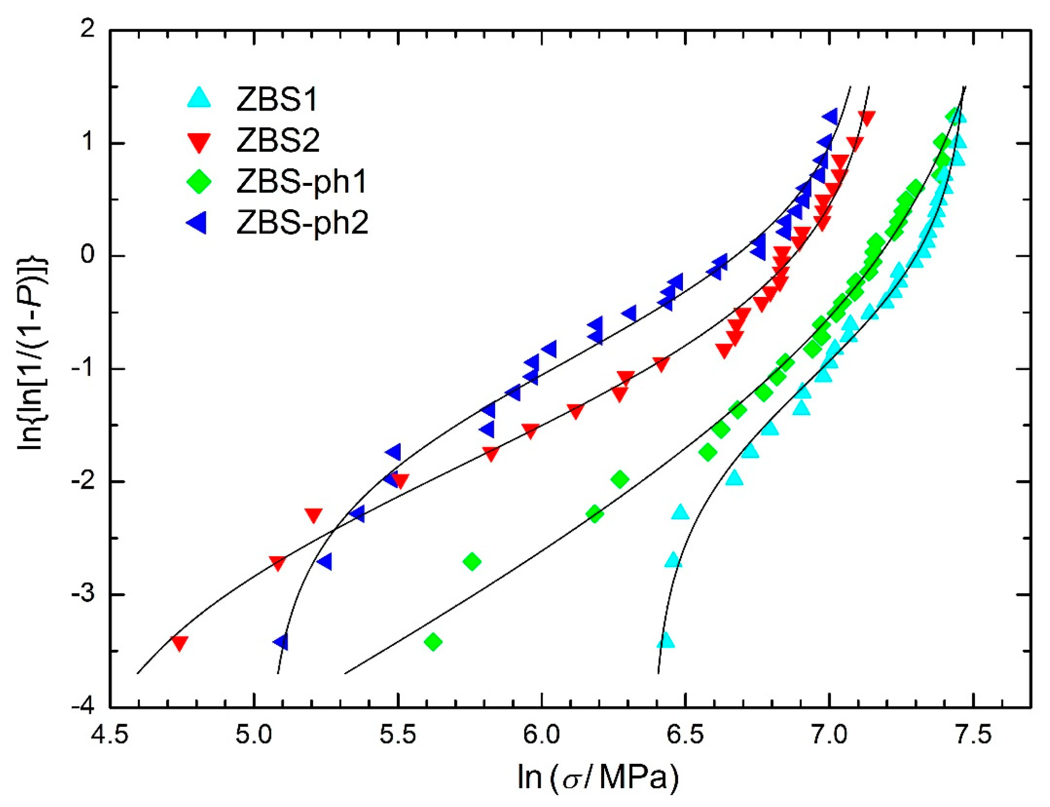
The strength degradation of SiC fibers with a porous ZrB2-SiC coating was studied by Wu et al. [5]. Silicon carbide fibers are widely used as a reinforcement of ceramic-matrix composites due to their low coefficient of thermal expansion, low density, good thermal shock resistance, and excellent high-temperature strength. The toughness of composites depends on the fiber-matrix interfacial layers realized by fiber coating. On the other hand, the porosity of the coating decreases the strength of fibers, which was the main topic of the paper [5]. The four variants of ZrB2-SiC coating were applied, designated as ZBS1, ZBS2, ZBS-ph1, and ZBS-ph2 (for their description, see [5]). Figure 8 shows the Weibull plot of the tensile strength of coated SiC fibers with the Weibull failure probability estimator (4). The authors talk about the bimodal Weibull distribution, but it seems to be mostly trimodal and, according to the course of the curves in Figure 8, the regression function (W4) describes all curves very well except for the curve for ZBS-ph1 coating, which is curved only once. The regression calculations give the following values of σ0 and σ strength: 591 MPa and 1790 MPa for the ZBS1 coating, 74 MPa and 1326 MPa for the ZBS2 coating, and 155 MPa and 1263 MPa for the ZBS-ph2 coating. For the ZBS-ph1 coating, only the value σ = 2138 MPa could be calculated. It can be formally written as σ0 = 0 MPa for this coating if the regression function (W4) is used, or the three-parameter Weibull distribution with upper limit (W3max) can be applied (see also [4]).

3.3. Fatigue of FeE 460 Steel

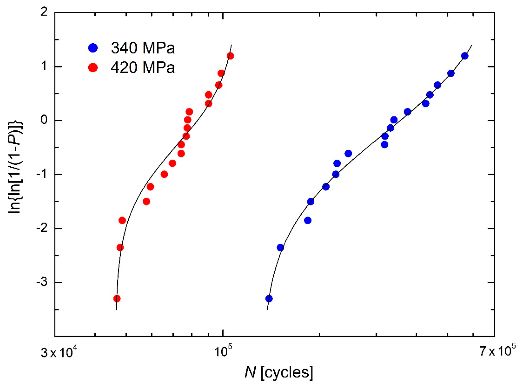
Fatigue investigation of the typically welded joints in FeE 355 and FeE 460 types of steel was made by Haibach et al. [13]. The number of cycles to fracture for the FeE 460 steel loaded with σmax = 340 MPa and 420 MPa at loading cycle asymmetry ratio R = 0.1 together with the failure probability estimator
P i = 3 i 1 3 n + 1 = i 1 / 3 n + 1 / 3
is shown as the Weibull plot in Figure 9. Using the regression function (W4) leads to the following numbers of cycles to fracture N0 and N: 131 × 103 and 761 × 103 cycles for 340 MPa and 46 × 103 and 111 × 103 cycles for 420 MPa.

3.4. Flexural Fatigue of Concrete

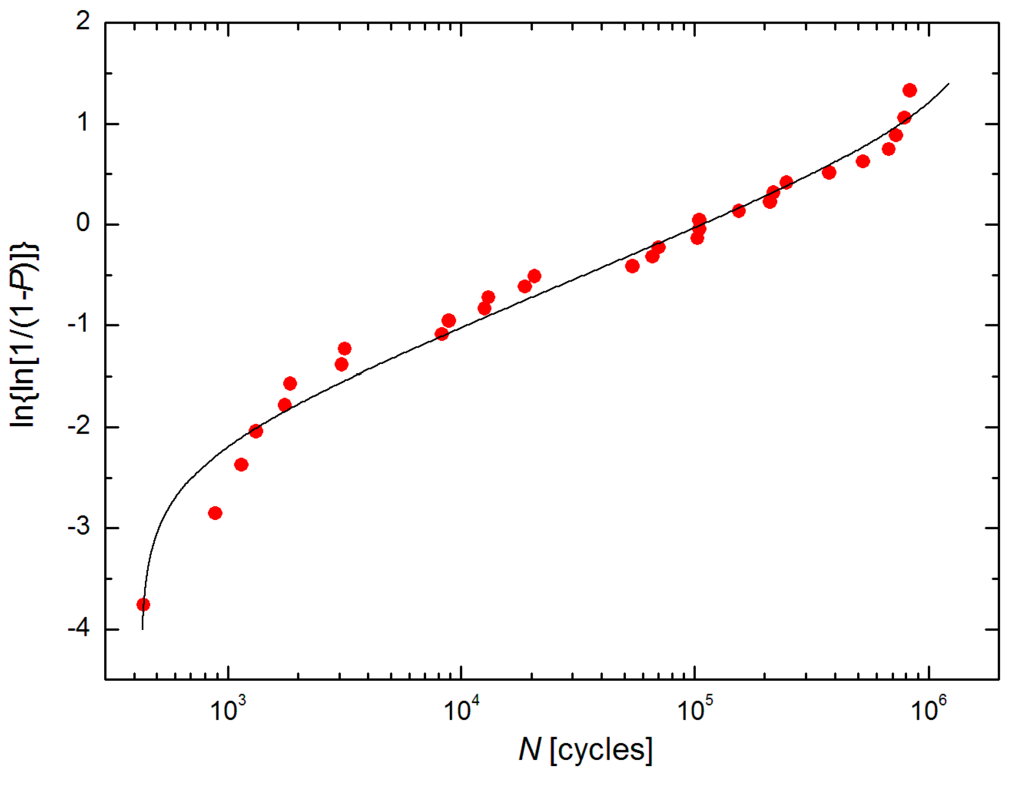
The influence of aggregate size on the flexural fatigue response of concrete was studied by Kasu et al. [14]. The test specimens of 100 mm × 100 mm × 500 mm size were prepared with a blend of fine aggregate and coarse aggregate with nominal maximum aggregate sizes of 10 mm (S10) and 20 mm (S20). The specimens made of both mixtures (S10 and S20) were tested in four-point bending at the frequencies of 2, 5, and 10 Hz and at the maximum stresses corresponding to 80, 85, and 90% of their flexural strength. The Weibull plot in Figure 10 is drawn for the fatigue life (the number of cycles to fracture) of the S10 specimens loaded with the flexural stress of 3.828 MPa (90% of the flexural strength) at the frequency of 2 Hz. The relation for failure probability Pi is not specified in the paper [14], but the Weibull plots in this paper indicate that the Benard approximation (5) was used. Using the regression function (W4) leads to the number of cycles to fracture N0 = 428 cycles and N = 1.935 × 10⁶ cycles. The authors [14] considered the three-parameter Weibull distribution, and using the maximum likelihood method, they estimated the value of the location (threshold) parameter to be 216 cycles (i.e., approximately N0/2).

3.5. Surface Defects of a Sandblasted Glass

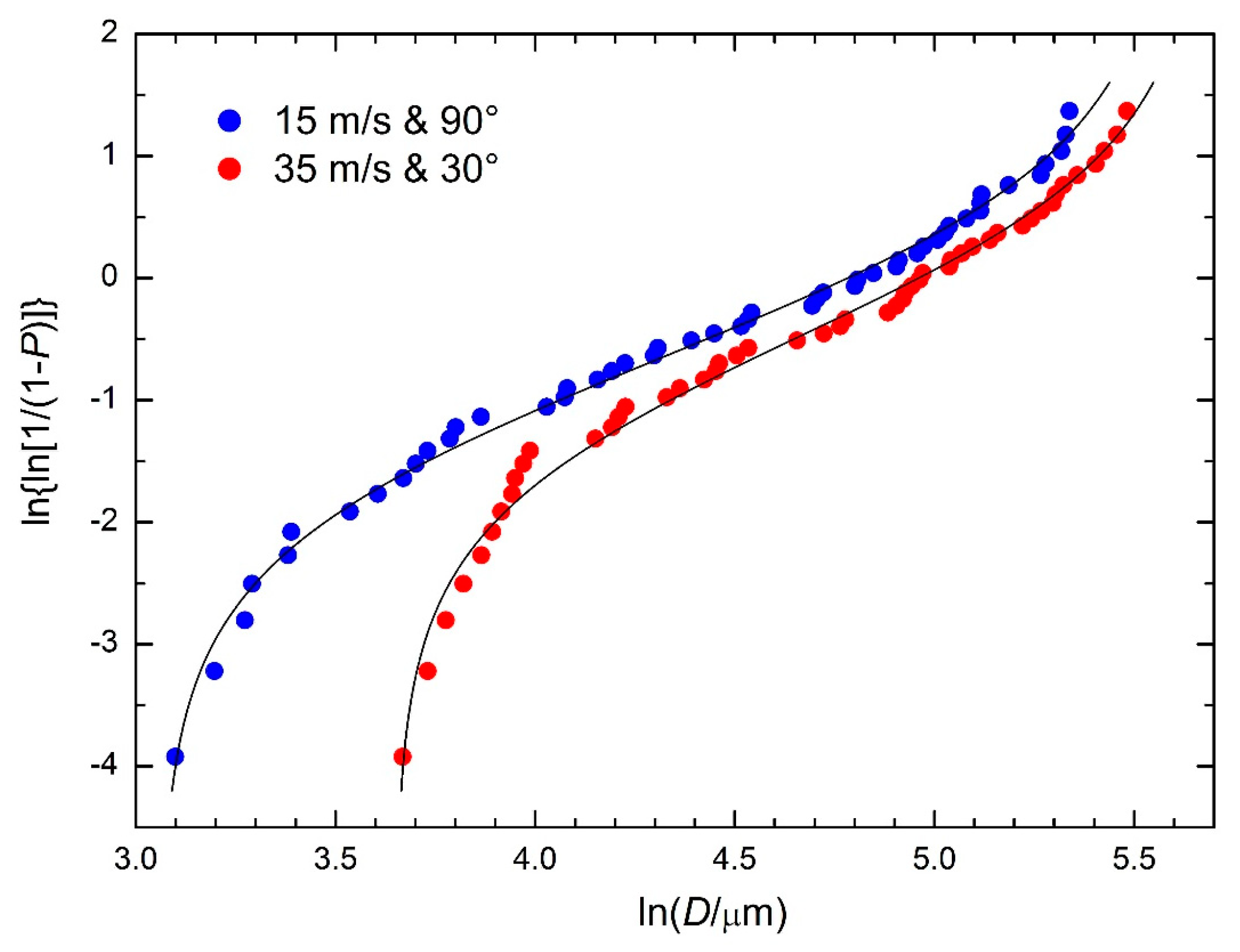
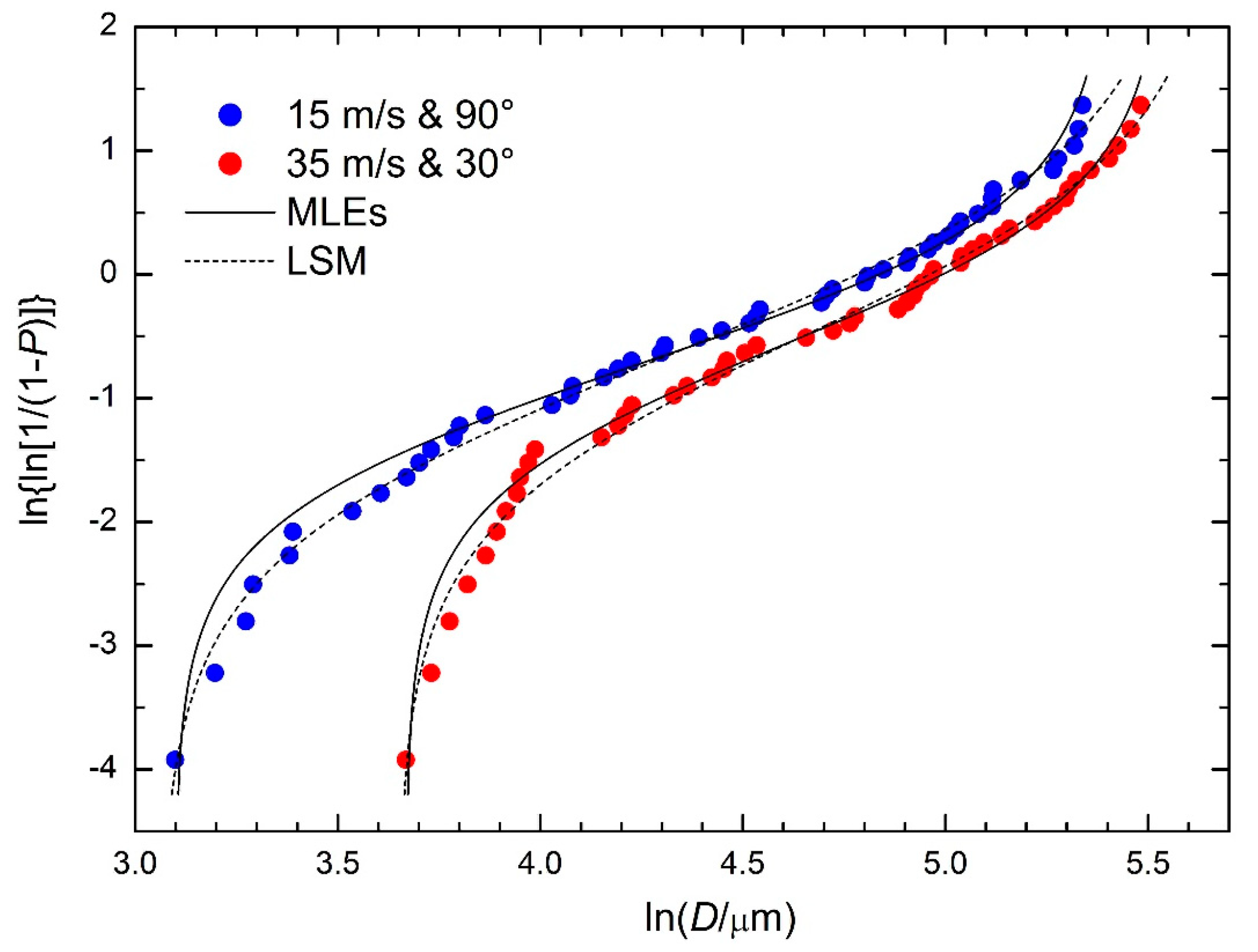
Sandblasting erosion tests simulating the effect of sandstorms in the Saharan regions on soda lime glass were performed by Barka et al. [15]. The influence of three different velocities of sand particles and three different impact angles on the defect sizes and defect numbers was studied. The defect size distribution was identified as the Weibull distribution for the conditions (15 m/s and 90°) and (35 m/s and 30°) as the bimodal Weibull distribution [15]. The Weibull plot of the defect sizes for the mentioned conditions with the Weibull failure probability estimator (4) is drawn in Figure 11. The trimodal Weibull distribution also offers consideration here but using the regression function (W4) leads to a better fit even with fewer parameters and a smooth regression curve. The regression calculations give D0 = 21.4 μm and D = 267 μm for (15 m/s and 90°) conditions and D0 = 38.5 μm and D = 291 μm for (35 m/s and 30°) conditions.

4. Distribution Parameters Determined by MLEs

In addition to the above applied least squares method (LSM), the maximum likelihood estimations (MLEs) are often used for the determination of the distribution parameters. For the (W4) CDF, the maximum of the term
ln L ( η , β , t 0 , t ) = n [ ln β + ln ( t t 0 ) + β ( ln t ln η ) ] + ( β 1 ) A ( β + 1 ) B ( t η ) β C
where n is the number of values in the studied data set and
A = i = 1 n ln ( t i t 0 ) ,   B = i = 1 n ln ( t t i ) ,   and   C = i = 1 n ( t i t 0 t t i ) β
is being sought to determine the parameter values η, β, t0, and t. For maximization, also the SOLVER supplement in MS Excel can be used. The MLEs of the distribution parameters are not dependent on the relations for the Pi values of cumulative probability (see Equations (3) to (6)). On the other hand, it is well known that the MLEs of the parameters are usually noticeably biased. For comparison of the Weibull plots based on the parameters determined using the LSM (for both the extreme a values are 0 and 0.5) and the MLEs, the data from Figure 11 were used (many empirical points with relatively low dispersion). The result of the comparison is shown in Figure 12 and in Table 2. While the values of parameters determined using the LSM are numerically distinguishable when Equations (3) or (4) are used for Pi calculations (see Table 2), the corresponding curves are not graphically distinguishable (see dashed lines in Figure 12 representing both cases).
Comparison of the curves in Figure 12 and the parameter values in Table 2 for both LSM and MLEs approaches shows that the corresponding curves are relatively close even at significantly different parameter values. Generally, it means that a significant covariance of regression parameters exists. Figure 12 also shows a general tendency mentioned already in the previous paper [4]: the LSM fits are better for the lower values of the independent variable, while the MLEs fits are better for the higher values of the independent variable, especially the upper arcs are captured very accurately.

5. CDF with a Greater Number of Parameters

The problems with the physical dimension and physical unit of the α parameter in the Phani modification (13) were already described in the Section 1. These problems can be eliminated by introducing a new parameter η given by the relation
η = ( t β 2 α ) 1 / β 1 .
Then, the Phani modification (13) can be written in the form of
P ( t ) = 1 exp [ ( t η ) β 1 ( 1 t 0 t ) β 1 ( 1 t t ) β 2 ]
where no problems with dimensions or units appear. However, now the question arises why two of the brackets in Equation (27) have the same exponent, and the third bracket has a different one. For three generally different exponents, β1, and β2, the six-parameter Weibull CDF can be written as
P ( t ) = 1 exp [ ( t η ) β ( 1 t 0 t ) β 1 ( 1 t t ) β 2 ]
where (when displayed as the Weibull plot) the η parameter describes the position of the middle straight part, the parameter β describes its slope, the t0 and t parameters describe the positions of the left and the right bend, respectively, and the β1 and β2 parameters describe their curvatures. For β1 = β2 = β, the (W6) CDF is simplified into the (W4) CDF.
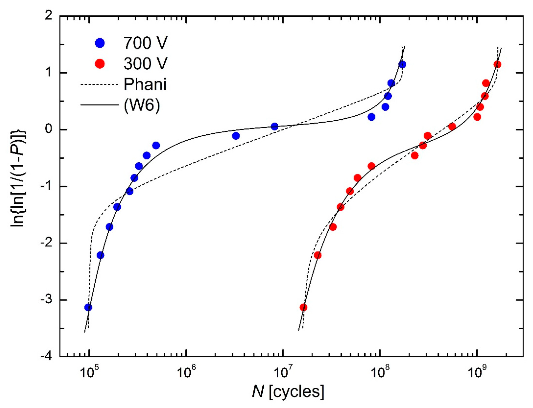
The best data sets for the application of the (W6) CDF with a greater number of parameters seem to be those atypical sets in Figure 6: the numbers of cycles to the destruction of the multilayer ceramic piezoelectric actuators at the temperature of 90 °C for 300 V and 700 V AC biases [11]. In Figure 13, the 5-parameter Phani modification (dashed lines) and 6-parameter (W6) modification (solid lines) are used. It can be clearly seen that the (W6) CDF leads to substantially better fits than the Phani CDF. The regression procedure for the 700 V data set is as follows:
  • using the (W4) CDF was fully unstable; therefore, the firmly given values N0 = 9.79 × 10⁴ cycles (closely below the minimum number of cycles) and N = 1.71 × 10⁸ cycles (closely above the maximum number of cycles) had to be used (see Figure 6),
  • using the Phani CDF was stable, but the fit was not acceptable (see the left dashed line in Figure 13),
  • using the (W6) CDF was stable, and the fit was fully acceptable (see the left solid line in Figure 13).
The regression procedure for the 300 V data set was stable in all these three cases, but only the (W6) CDF led to fully acceptable fit (see the right solid line in Figure 13).
The sums of least squares for the data sets from Figure 6 (or Figure 13) using the (W4) CDF, the Phani modification, and the (W6) CDF are presented in Table 3. The substantial decreases in the sums of least squares were very conspicuous when the 5-parameter Phani modification was replaced by the 6-parameter (W6) CDF.
Considering t >> t (or equivalently t → ∞), the (W6) CDF can be simplified as
P ( t ) = 1 exp [ ( t η ) β ( 1 t 0 t ) β 1 ]
which leads to the (W3min) CDF for β1 = β. Considering t0 << t (or equivalently t0 → 0), the (W6) CDF can be simplified as
P ( t ) = 1 exp [ ( t η ) β ( 1 t t ) β 2 ]
which leads to the (W3max) CDF for β2 = β. While the (W3min) and (W3max) CDFs are sufficient for the Weibull plots with smooth arcs, the (W4min) and (W4max) CDFs lead to substantially better fit in the cases, when slightly curved parts of the Weibull plots covert into sharper arcs (see the fits below).
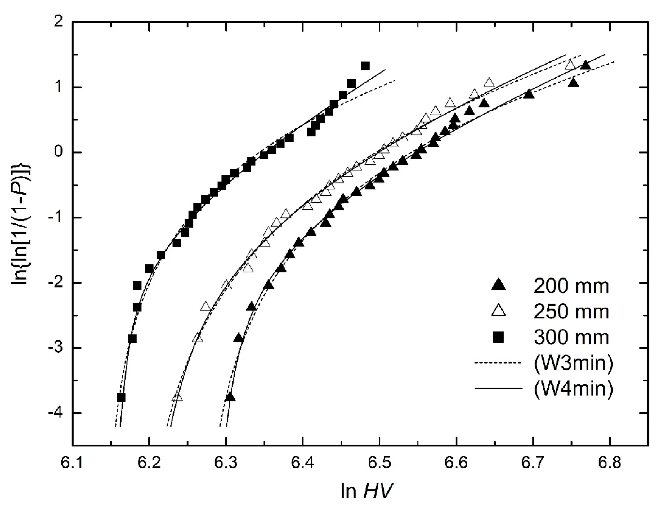
For the comparison of the fits based on the (W3min) and (W4min) CDFs, the data sets of Gan and Berndt [16] were used. They studied plasma sprayed Nd–Fe–B coatings on substrates made of 304 austenitic stainless steel, including their mechanical properties, and, assuming the bimodal Weibull distribution, they fitted the Weibull plots of Vickers microhardness with two straight lines. In the previous paper [4], it was shown that the (W3min) CDF leads to substantially better fits than the bimodal Weibull distribution, and Figure 14 shows the comparison of the fits based on the (W3min) and (W4min) CDFs. At first glance, it can be said that using the (W4min) CDF leads for all three standoff distances of 200 mm, 250 mm, and 300 mm:
  • to better fit generally,
  • to better fit all parts of the Weibull plot,
  • to smaller curvature of the part of the curve with small curvature (almost a straight-line part, see upper parts of solid lines),
  • to bigger curvature of the arc of the curve (see lower parts of solid lines),
  • to a higher value of the t0 parameter.
The first and the last item can be expressed numerically (see Table 4). Here it can be seen that the sum of least squares S decreased by 13 to 46%, which is a decrease worthy of consideration. The increase in the t0 parameter is between 9 and 14 HV i.e., between 2 and 3%.
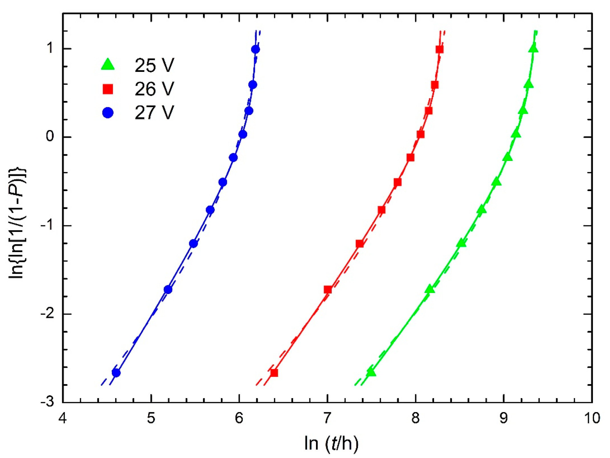
For the comparison of the fits based on the (W3max) and (W4max) CDFs, the times to failure determined for a power transistor tested at three voltages, 25 V, 26 V, and 27 V (see EN 62506 [17], Annex G), were used. The curves corresponding to both CDFs are nearly identical (excluding the ends of the curves, see Figure 15), but a careful look shows that the fitting curves corresponding to the (W4max) CDF pass through the empirical points with extraordinary precision. Therefore, the sum of least squares decreases in a fundamental way (by 94 to 97%, see Table 5), and the decrease in the values of the t parameter is also significant (by 12 to 20%, see also Table 5).

6. Discussion

6.1. Modular form of the (W6) CDF

The expression in the brackets in Equation (W6) (not considering the minus sign) can be schematically written as
MSL × LB UB
where MSL means the middle straight-line part, LB means the lower bend, and UB means the upper bend of the corresponding Weibull plot. Each of the two bends can be replaced by 1 in Equation (28) when it is not part of the studied Weibull plot. Then, the Weibull plots can be symbolically described by the schemes
MSL ,   MSL × LB   or   MSL UB
when the plot is without the bends, the plot with the lower bend or the plot with the upper bend are considered, respectively. The first scheme in Equation (29) corresponds to the (W2) CDF; the second scheme corresponds to the (W4min) CDF, and, finally, the third scheme corresponds to the (W4max) CDF. All written here about the (W6) CDF is also valid for the (W4) CDF, formally rewritten in the form of
P ( t ) = 1 exp [ ( t η ) β ( 1 t 0 t ) β ( 1 t t ) β ]
((W6) CDF simplifies to (W4) CDF when β1 = β2 = β, as mentioned above) where the schemes in Equation (29) represent the (W2), (W3min), and (W3max) CDFs, respectively.
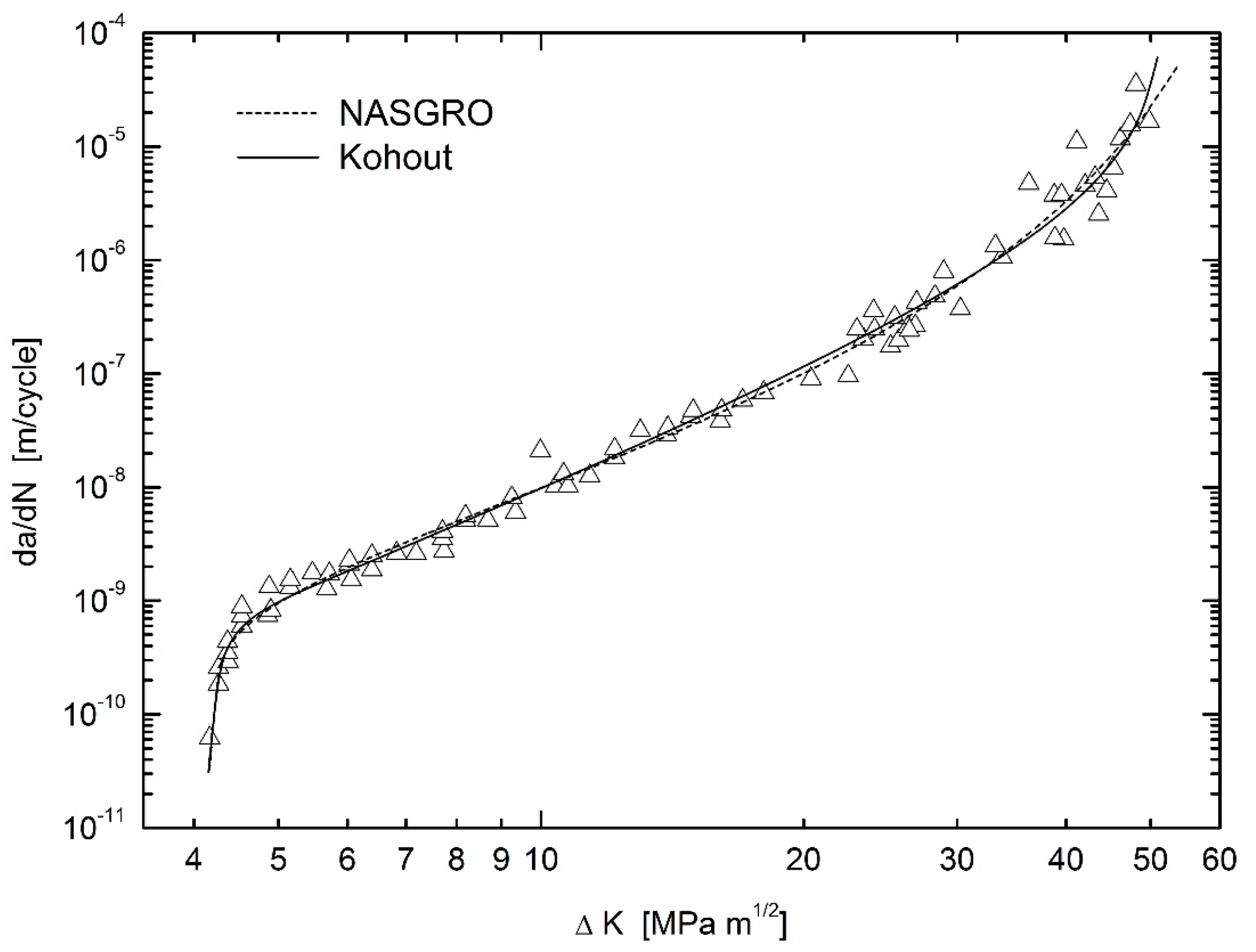
Equation (W6) is formally very similar to the NASGRO equation describing the growth of fatigue cracks [18] (see Equation (2.8) in [18] written for pulsating-tension loading)
d a d N = C Δ K n ( 1 Δ K th Δ K ) p ( 1 Δ K K c ) q
where N is the number of applied fatigue cycles, a is the crack length, ΔK is the stress intensity factor range, ΔKth is the threshold stress intensity factor range, Kc is the critical stress intensity factor, C, n, p, and q are empirically derived constants. Parallel to Equation (28), the right side of Equation (30) (not considering constant C) can be schematically written as
SCP × CI ICP
where SCP means the stable crack propagation (according to the Paris law), CI means the crack initiation, and ICP means the unstable crack propagation. CI or ICP can be replaced by 1 in Equation (31) when it is not part of the studied curve of fatigue crack propagation. Then, these curve plots can be symbolically described by the schemes
SCP ,   SCP × CI   or   SCP ICP
when (i) the plot of the stable crack propagation (without both the crack initiation and the unstable crack propagation), (ii) the plot of the stable crack propagation with the crack initiation, or (iii) the plot of the stable crack propagation with the unstable crack propagation are considered, respectively. The first scheme in Equation (31) corresponds to the Paris law
d a d N = C Δ K n
etc. All mentioned above shows a big formal similarity between Equations (W6), (W4a), and the NASGRO equation (see Equation (30)). Less similarity, but the same modular form (see Equation (28) or (31)) is also found in the equation (see Equation (24) in the author’s paper [19], formally converted)
d a d N = C Δ K n 1 ( Δ K th Δ K ) p 1 ( Δ K K c ) q
describing the growth of fatigue cracks as well as Equation (30) (the meaning of variables and parameters is analogical to those in Equation (30)). The empirical fatigue crack growth curve for austempered ductile cast iron [20] with a grain size of 84 mm loaded at loading cycle asymmetry ratio R = 0.1 was fitted using Equations (30) and (34) as regression functions (see Figure 16). Its double-curved form is principally the same as the form of the double-curved Weibull plots (see Figure 1 and Figure 5, Figure 6, Figure 7, Figure 8, Figure 9, Figure 10, Figure 11, Figure 12, Figure 13).

6.2. Upper and Lower Limitations of Data Sets in Reliability Studies and Material Testing

The upper limitation of a lifetime can be subconsciously understood (nothing lasts in the world forever—is sung in a Czech song). The upper limitation of mechanical properties is derived from the maximum theoretical strength of metal single crystals (approx. one-tenth of the tensile modulus of elasticity). Structural materials that are commercially produced for engineering applications commonly fracture at applied stress levels 10 to 100 times below this value due to stress concentrators (cracks and notches) and due to planes of weakness (grain boundaries in polycrystalline materials) [21]. Analogical considerations are also possible for non-metallic materials. On the other hand, in some cases, limited maximum values are required e.g., the maximum of the material strength when protective equipment and work clothes are considered (the sleeve caught by the rotating spindle of the lathe must have limited strength to avoid serious injury to the lathe operator).
The lower limitation of data sets in reliability studies and material testing is a rather more complex phenomenon. Entities (parts, products, etc.) or materials for their production with the lowest properties are eliminated in the pre-production phase, during the production process itself, during production checks, during final inspection, and, often, also during the selection of samples for tests. E.g., test bars for mechanical tests made of (very) low-strength material may be destroyed during production and will not be subjected to mechanical tests at all; microelectronic components may be discarded prior to testing during verification of their functionality, etc. These eliminations can be carried out by the production operator consciously or unconsciously, or independent of him/her. Most of them are carried out without known or fixed limits; therefore, neither a censored nor a truncated distribution can be applied. On the other hand, Kasu et al. [14] excluded from statistical processing the samples that failed at less than 100 bending cycles (it deals with the S20 concrete specimens not studied in this paper); it can be spoken of as a censored sample in this case.
The two-side limitation of data sets can also occur due to the nature of the measured quantity. The data set of the surface defect lengths in the sandblasted glass studied by Barka et al. [15] may be principally truncated on both sides: very short defects may not be observable, very long defects can lead to fracture before they can be measured, and therefore, will not be included in the data set. In sum, the distribution with upper and lower limits (here, the (W4) CDF or, in specific cases, the (W6) CDF) corresponds to reality better than the theoretical (W2) distribution without limits). Nearly all figures in this paper show that the twice-curved Weibull plot can be successfully described by the (W4) CDF. There are only two exceptions:
  • the left curve in Figure 6, for which the regression calculations gave no meaningful values of the parameters t0 and t (here specifically N0 and N), and they had to be firmly given to obtain an “optically-acceptable” fit (but the (W6) CDF yields perfectly acceptable fit, see Figure 13),
  • the third curve (from the left) in Figure 8, which is significantly curved only once and not the (W4), but the (W3max) CDF is suitable in this case.

6.3. Bathtub-Shaped Hazard Rate Curve

In reliability studies, the bathtub-shaped hazard rate curve is very important; therefore, in the case of simple distributions, the piecewise model of the bathtub curve is usually used. For the (W2), (W3min), and (W4min) CDFs, no bathtub-shaped HR curve is obtained, but a compact bathtub-shaped HR curve is obtained if the upper t is introduced, i.e., for the (W3max), (W4), (W4max), and (W6) CDFs. For the simplest of them, i.e., for the (W3max) CDF, the hazard rate has its minimum value for tmin = (1 − β) t/2, but the inequality β < 1 must be valid [4]; for the (W4) CDF the position of the hazard rate minimum value is given by Equation (19), and the upper limit of the β parameter depends on the t/t0 ratio (see Equation (21)). In reliability studies, the β parameter values are usually small (especially if determined using MLEs), and the bathtub-shaped hazard rate curve is usually obtained for the (W3max), (W4), (W4max), and (W6) CDFs. In material testing, higher values of the β parameter are more usual, but here, the hazard rate has no significance. Generally, higher values of the β parameter in the (W2) CDF may be a symptom to consider the (W3min), (W3max), or (W4) CDF application, but a more reliable symptom is curved Weibull plot (concavely curved, convexly curved or twice curved, respectively).
Usually, the hazard rate is derived from the CDF using Equation (16). However, the opposite procedure is also possible: Zeng et al. [22] started from the Perks mortality equation [23] for bathtub-shaped hazard rate and derived the corresponding CDF from it. This results in a very complicated form of the CDF for the 4-parameter Perks function and an extremely complicated form of the CDF shape for the 5-parameter Perks function. On the other hand, the (W3max), (W4), (W4max), and (W6) CDFs can be written in relatively very simple forms, and the bathtub-shaped hazard rates derived from them have also relatively simple forms. In particular, the hazard rate curves derived from the (W4max) and (W6) CDFs containing 5 and 6 parameters, respectively, have an ability to adapt to the course of empirical hazard rate curve (see Figure 2 and Figure 3) that is comparable or even better than that of the Perks functions.

6.4. Optimum Number of Distribution Parameters

On the other hand, it should be emphasized that for a slight curvature of the Weibull plot, the original (W2) CDF should be preferred over both the (W3max) and (W3min) CDFs [4]. Similarly, the (W3max) CDF should be preferred over the (W4max) CDF, (W3min) over (W4min), (W4) over (W6), and sometimes also (W3max) over (W4) (see, e.g., the third curve in Figure 8), and (W3min) over (W4), unless there are compelling reasons to use more complex functions. Generally said, the more complex CDF (i.e., the regression function with a higher number of parameters) can be applied:
  • when the coefficient of determination noticeably increases or, equivalently, the residual sum of squares noticeably decreases,
  • when the relative standard deviations of the regression parameters do not reach tens of a percent (or more),
  • when the maximum likelihood value noticeably increases.
For smaller data sets (less than tens of empirical points), the adjusted coefficient of determination R ¯ 2
R ¯ 2 = 1 ( 1 R 2 ) n 1 n k 1
(where n is the sample size and k is the number of parameters) should be used instead of the usual coefficient of determination R2, and the residual sum of squares (sum of least squares) per degree of freedom s
s = S n k
should be used instead of the residual sum of squares S. Accurate decision-making must be based, for example, on the Akaike information criterion [24] (in the case of MLEs) or on analogical criteria suitable for LSM.

6.5. Curvature of the Weibull Plots

In the previous paper [4] also, the influence of the curvature of convexly curved Weibull plots on the standard deviation of the t parameter (included in the (W3max) CDF) was discussed. It was shown that this standard deviation substantially decreases with increasing curvature. As a simple measure of the curvature, the degree of curvature of the Weibull plot expressed as (η/t)1/β was suggested and verified. Analogously, for the curvature of concavely curved Weibull plots (described by the (W3min) CDF), the degree of curvature expressed as (t0/η)1/β can be considered (some initial studies showed a close relation between this curvature and the standard deviation of the t0 parameter). For the Weibull plots with both lower and upper limits (described by the (W4) CDF), both the degrees of curvature (t0/η)1/β and (η/t)1/β could be used. Their product (t0/t)1/β contains the reciprocal value of the k ratio (see Equation (21), 1/k = t0/t), which determines the upper limit of the β parameter values corresponding to the bathtub-shaped hazard rate connected with the (W4) CDF.

6.6. Other Authors’ CDFs with More Parameters

There are only two more widely cited modifications of the Weibull CDF with more than three parameters: the Kies modification [6] with four parameters (see Equation (11)) and the Phani modification [7] with five parameters (see Equation (12)). As shown above, the Kies modification is in principle equivalent to the newly derived (W4) CDF, where a very problematic and difficult-to-interpret parameter α is replaced by the η parameter (see Equation (15)) already included in the (W2), (W3max), and (W3min) CDFs. The Phani modification with five parameters represents a certain intermediate stage between the (W4) and (W6) CDFs, which (compared with the (W4) CDF) does not lead to a noticeably better fit, but improves the stability of the regression calculations (see Figure 13). The inconsistency of this intermediate step is evident in the form of notation in Equation (27), where two of the three exponents are equal. The natural requirement that all three exponents be different leads directly to the (W6) CDF with the ability to fit even very unusual courses of the Weibull plots (see also Figure 13).

6.7. Final Comment

As time progresses, more and more probability distributions are published, which (albeit mostly at the cost of complexity) better describe the specifics of data sets obtained under specific conditions. For example, very promising modifications of the decades-known Lindley distribution have been published recently, in particular the XLindley and power XLindlay distributions [25,26,27]. Among the enormous number of different new distributions, there would likely be some that would prove useful in some of the specific cases studied in this article. However, the author’s goal was not to search for the most suitable distribution for a given specific case from all published distributions but to supplement the classic two-parameter Weibull distribution W2, the commonly used three-parameter Weibull distribution with a lower limit W3min, and the three-parameter Weibull distribution with an upper limit of W3max introduced by the author [4] with a four-parameter Weibull distribution W4 with both of these limits. This results in a consistent quartet of distributions, where each distribution with more parameters can be simplified to a distribution with fewer parameters according to the schemes W4 → W3min → W2 and W4 → W3max → W2, as stated in the Section 1.

7. Conclusions

The presented findings can be summarized as follows:
  • The Weibull plots, which are somehow curved, are usually fitted with several straight lines. The concavely–convexly curved Weibull plots can be successfully fitted with the regression function described by Equation (W4) containing the lower limit t0 and the upper limit t of the independent variable. This equation can be especially useful in reliability studies and material testing.
  • In the field of reliability, the t0 and t parameters can be called minimum and maximum lifetime (time to failure, time-to-breakdown, etc.). In material testing, they can be called minimum and maximum strength (fracture toughness, defect size, etc.). In the fatigue of materials, the t parameter can mean the number of cycles to fracture.
  • The hazard rate curves corresponding to the (W4) CDF are bathtub-shaped (with the minimum hazard rate for the tmin = (1 + β) t0/2 + (1 − β) t/2 value) not only for β < 1 (as in the case of the (W3max) CDF) but also for the greater values of the β parameter. Their limitation depends on the t/t0 ratio.
  • In most cases of reliability studies described by the (W4) CDF, the values of the β parameter are small enough (especially if they are determined using the MLEs) to obtain bathtub-shaped hazard rate curves. In material testing, higher values of the β parameter are more usual, but here, the hazard rate has no specific significance.
  • It turns out that there seems to be a certain border area between the decreasing HR and the bathtub-shaped HR, where different criteria (hazard rate dependence versus TTT plot) give different qualitative results (whether the decreasing or the bath-tub shaped HR).
  • In the cases of data sets, when longer straight parts of their Weibull plots convert into sharper arcs, the CDFs with the higher number of parameters can be successfully used: (W4max) instead of (W3max), (W4min) instead of (W3min), and (W6) instead of (W4). It is valid, especially for big data sets with limited dispersion.
  • All presented CDFs are fully consistent with the (W2) CDF describing the straight-line Weibull plot. The Kies modification, as published, is not consistent with the (W2) CDF but can be rewritten into a fully consistent form, which is fully equivalent to the (W4) CDF. The Phani modification with five parameters is not consistent with the (W2) CDF. It represents a certain intermediate stage between the (W4) and (W6) CDFs and usually does not lead to a noticeably better fit than the (W4) CDF. Its application is questionable.

Funding

This research received no external funding.

Institutional Review Board Statement

Not applicable.

Informed Consent Statement

Not applicable.

Data Availability Statement

Not applicable.

Acknowledgments

Financial support from the Ministry of Defence of the Czech Republic within the Long-term Project for the Development of the Organization “DZRO Military autonomous and robotic systems” is gratefully acknowledged. In addition, the author is grateful to all authors, whose original experimental results were used in this paper.

Conflicts of Interest

The author declares no conflict of interest.

References

  1. Weibull, W. A Statistical Distribution Function of Wide Applicability. J. Appl. Mech. 1951, 18, 293–297. [Google Scholar] [CrossRef]
  2. Weibull, W. A Statistical Theory of the Strength of Materials; Generalstabens litografiska anstalts förlag: Stockholm, Sweden, 1939. [Google Scholar]
  3. Benard, A.; Bos-Levenbach, E.C. Het uitzetten van waarnemingen op waarschijnlijkdeids-papier (The Plotting of Observations on Probability Paper). Stat. Neerl. 1953, 7, 163–173. [Google Scholar] [CrossRef] [Green Version]
  4. Kohout, J. Three-parameter Weibull distribution with upper limit applicable in reliability studies and materials testing. Microelectron. Reliab. 2022, 137, 114769. [Google Scholar] [CrossRef]
  5. Wu, B.; Ni, N.; Fan, X.; Zhao, X.; Xiao, P.; Guo, F. Strength degradation of SiC fibers with a porous ZrB2-SiC coating: Role of the coating porous structure. J. Eur. Ceram. Soc. 2019, 40, 961–971. [Google Scholar] [CrossRef]
  6. Kies, J.A. The Strength of Glass; Report No. 5093; Naval Research Laboratory: Washington, DC, USA, 1958. [Google Scholar]
  7. Phani, K.K. A new modified Weibull distribution function. J. Am. Ceram. Soc. 1987, 70, 182–184. [Google Scholar] [CrossRef]
  8. Atanassova, E.; Novkovski, N.; Spassov, D.; Paskaleva, A.; Skeparovski, A. Time-dependent-dielectric-breakdown characteristics of Hf-doped Ta2O5/SiO2 stack. Microelectron. Reliab. 2014, 54, 381–387. [Google Scholar] [CrossRef]
  9. Aarset, M.V. How to Identify a Bathtub Hazard Rate. IEEE Trans. Reliab. 1987, 36, 106–108. [Google Scholar] [CrossRef]
  10. Marcon, D.; Meneghesso, G.; Wu, T.; Stoffels, S.; Meneghini, M.; Zanoni, E.; Decoutere, S. Reliability Analysis of Permanent Degradations on AlGaN/GaN HEMTs. IEEE Trans. Electron. Devices 2013, 60, 3132–3141. [Google Scholar] [CrossRef]
  11. Jung-Hyuk Koh, Tae-geun Kim, Reliability of Pb(Mg, Nb)O3-Pb(Zr, Ti)O3 multilayer ceramic piezoelectric actuators by Weibull method. Microelectron. Reliab. 2006, 46, 183–188. [CrossRef]
  12. Wei, S.; Xie, Z.; Xue, W.; Yi, Z.; Chen, J.; Cheng, L. Strengthening mechanism of aluminum nitride ceramics from 293 to 77 K. Mater. Lett. 2014, 119, 32–34. [Google Scholar] [CrossRef]
  13. Haibach, E.; de Back, J.; Lieurade, H.P.; Olivier, R.; Rinaldi, F.; Simon, P. Fatigue Investigation of Typical Welded Joints in Steel FeE 460 as Compared to FeE 355 (Final Report); Office for Official Publications of the European Communities: Luxembourg, 1979; Available online: https://op.europa.eu/cs/publication-detail/-/publication/abc108c7-e101-4e94-a58e-71a08af10a96/language-en (accessed on 7 December 2022).
  14. Kasu, S.R.; Deb, S.; Mitra, N.; Muppireddy, R.A.; Kusam, S.R. Influence of aggregate size on flexural fatigue response of concrete. Constr. Build. Mater. 2019, 229, 116922. [Google Scholar] [CrossRef]
  15. Barka, B.; Faci, A.; Bouaouadja, N.; Bousbaa, C.; Benachour, D.; Fatmi, M. Influence of the velocity and impact angle on the distribution of the surface defects of a sandblasted glass. Int. J. Appl. Glass Sci. 2018, 9, 471–479. [Google Scholar] [CrossRef]
  16. Gan, J.A.; Berndt, C.C. Effects of standoff distance on porosity, phase distribution and mechanical properties of plasma sprayed Nd–Fe–B coatings. Surf. Coat. Technol. 2013, 216, 127–138. [Google Scholar] [CrossRef]
  17. EN 62506:2013; Methods for Product Accelerated Testing (IEC 62506:2013). European Standardization Organization: Brussels, Belgium, 2013.
  18. Forman, R.G.; Shivakumar, V.; Mettu, S.R.; Newman, J.C. Fatigue Crack Growth Computer Program ‘NASGRO’ Version 3.0; Reference Manual JSC-22267B, NASA/Lyndon B; Johnson Space Center: Houston, TX, USA, 2000. [Google Scholar]
  19. Kohout, J. A new function describing fatigue crack growth curves. Int. J. Fatigue 1999, 21, 813–821. [Google Scholar] [CrossRef]
  20. Bartosiewicz, L.; Krause, A.R.; Kovacs, B.; Putatunda, S.K. Fatigue Crack Growth Behavior of Austempered Ductile Cast Iron. AFS Trans. 1992, 100, 135–142. [Google Scholar]
  21. Sun, C.T.; Jin, Z.-H. Fracture Mechanics; Elsevier: Amsterdam, The Netherlands, 2012. [Google Scholar]
  22. Zeng, H.; Tian, L.; Chen, Q. Five and four-parameter lifetime distributions for bathtub-shaped failure rate using Perks mortality equation. Reliab. Eng. Syst. Saf. 2016, 152, 307–315. [Google Scholar] [CrossRef]
  23. Perks, W. On some experiments in the graduation of mortality statistics. J. Inst. Actuar. 1932, 63, 12–57. [Google Scholar] [CrossRef]
  24. Akaike, H. A New Look at the Statistical Model Identification. IEEE Trans. Automat. Contr. 1974, 19, 716–723. [Google Scholar] [CrossRef]
  25. Beghriche, A.; Zeghdoudi, H.; Raman, V.; Chouia, S. New polynomial exponential distribution: Properties and applications. Stat. Transit. New Ser. 2022, 23, 95–112. [Google Scholar] [CrossRef]
  26. Gulzar, M.; Meriem, B.; Gemeay, A.M.; Almetwally, E.M.; Zeghdoudi, H.; Alshawarbeh, E.; Abdulrahman, A.T.; El-Raouf, M.M.A. Hussam, E. The Power XLindley Distribution: Statistical Inference, Fuzzy Reliability, and COVID-19 Application. J. Funct. Spaces 2022, 2022, 9094078. [Google Scholar]
  27. Metiri, F.; Zeghdoudi, H.; Ezzebsa, A. On the Characterisation of X-Lindley Distribution by Truncated Moments: Properties and Application. Oper. Res. Decis. 2022, 32, 97–109. [Google Scholar]
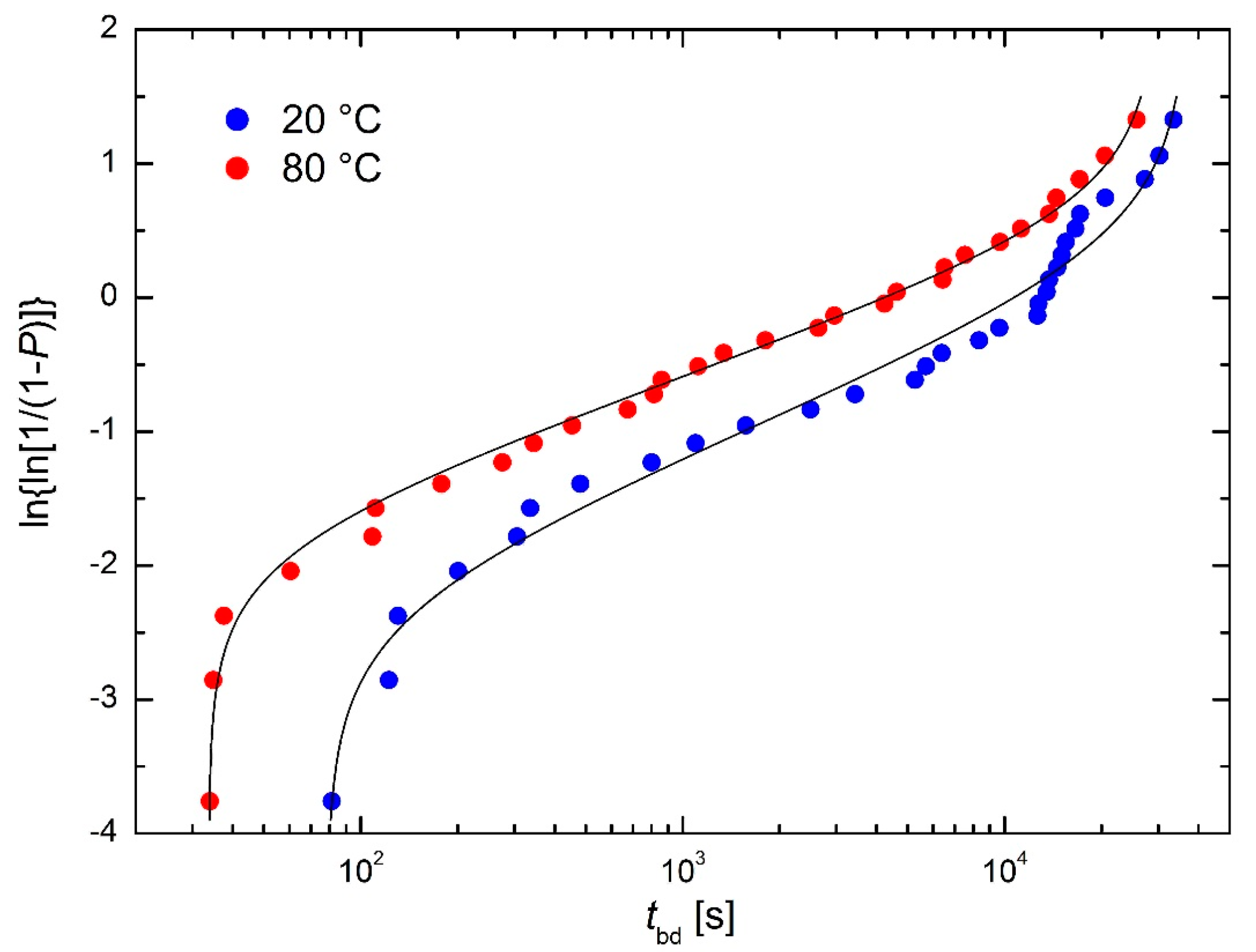
Figure 1. Weibull plots of the time-to-breakdown of Hf-doped Ta2O5/SiO2 capacitors under stress voltage −4.5 V at the presented temperatures [8].
Mathematics 11 00544 g001
Figure 2. Hazard rate (see Equation (17)) for the CDF (W4) of the time-to-breakdown of Hf-doped Ta2O5/SiO2 capacitors under stress voltage −4.5 V at the temperature of 80 °C [8], where the distribution parameters are determined by the LSM of the Weibull plot in Figure 1 (dashed line). Empirical HR is added (full circles) with its fit using Equation (17) (solid line).
Mathematics 11 00544 g002
Figure 3. Figure 2 in a more suitable log–log plot.
Mathematics 11 00544 g003
Figure 4. TTT plot of the time-to-breakdown of Hf-doped Ta2O5/SiO2 capacitors under stress voltage −4.5 V at the presented temperatures [8].
Mathematics 11 00544 g004
Figure 5. Weibull plots of the time-to-breakdown of GaN-based HEMTs at the temperature of 298 K for three gate voltages of −55 V, −60 V, and −65 V [10].
Mathematics 11 00544 g005
Figure 6. Weibull plots of the number of cycles to the destruction of the multilayer ceramic piezoelectric actuators at the temperature of 90 °C and the humidity of 30 % for given AC biases [11].
Mathematics 11 00544 g006
Figure 7. Weibull plots of the flexural strength of the aluminum nitride ceramic samples tested at given temperatures [12].
Mathematics 11 00544 g007
Figure 8. Weibull plots of the tensile strength of coated SiC fibers with given variants of ZrB2-SiC coating [5]. Regression function (W4) was successfully applied except for the ZBS-ph1 coating with σ0 = 0 MPa.
Mathematics 11 00544 g008
Figure 9. Weibull plots of the number of cycles to fracture for the FeE 460 steel cyclically loaded with σmax = 340 MPa and 420 MPa [13].
Mathematics 11 00544 g009
Figure 10. Weibull plot of fatigue life (the number of cycles to fracture) for the S10 concrete specimens loaded with the maximum flexural stress of 3.828 MPa at the frequency of 2 Hz [14].
Mathematics 11 00544 g010
Figure 11. Weibull plots of defect sizes in soda lime glass due to the air stream with sand particles at given velocities and impact angles [15].
Mathematics 11 00544 g011
Figure 12. Weibull plots of defect sizes in soda lime glass due to the air stream with sand particles at given velocities and impact angles [15] with the distribution parameters determined by MLEs (solid lines) and by LSM (dashed lines).
Mathematics 11 00544 g012
Figure 13. Weibull plots of the numbers of cycles to the destruction of the multilayer ceramic piezoelectric actuators at the temperature of 90 °C for given AC biases [11] for the 5-parameter Phani modification (dashed lines) and 6-parameter (W6) modification (solid lines).
Mathematics 11 00544 g013
Figure 14. Weibull plots for Vickers hardness of Nd–Fe–B coatings plasma sprayed from the 200 mm, 250 mm, and 300 mm standoff distances [16] using the (W3min) and (W4min) CDFs.
Mathematics 11 00544 g014
Figure 15. Weibull plots of the times to failure of a power transistor at the voltages 27 V, 26 V, and 25 V [17] for the (W4max) CDF (solid lines) and the (W3max) CDF (dashed lines).
Mathematics 11 00544 g015
Figure 16. Curve of fatigue crack growth for austempered ductile cast iron [20] with a grain size of 84 mm loaded at loading cycle asymmetry ratio R = 0.1. Regression functions (30) (dashed line) and (34) (solid line) were used for fits.
Mathematics 11 00544 g016
Table 1. Parameters of the (W4) CDF determined from the Weibull plot and empirical HR fit supplemented by the positions of the minima of the HR curves and the limit values of the β parameter.
Equationη [s]βt0 [s]t [s]tmin [s]h(tmin) [s−1]βmax
(W4)49410.84933.7529,20422322.247 × 10−41.002
(17)47220.43734.0833,86395491.005 × 10−41.002
Table 2. Comparison of the values of the distribution parameters of defect sizes in soda lime glass due to the air stream with sand particles at given velocities and impact angles [15] determined by MLEs and by LSM (two Equations (3) and (4) for cumulative probability values were considered).
Method →MLEsLSM
conditionsparameterEquations (24) and (25)a = 0 (Equation (4))a = 0.5 (Equation (3))
15 m/s and 90°η [μm]243.8177.9174.0
β [-]0.5760.7480.804
D0 [μm]22.221.421.8
D [μm]220.7266.7264.5
35 m/s and 30°η [μm]260.1205.1202.0
β [-]0.5900.7240.751
D0 [μm]39.238.538.8
D [μm]253.3290.7288.8
Table 3. Sums of least squares for the Weibull plots of the numbers of cycles to the destruction of the multilayer ceramic piezoelectric actuators at the temperature of 90 °C for given AC biases [11] when the (W4) CDF, the Phani modification, and the (W6) CDF were used as regression functions.
EquationParameters300 V700 V
(W4) ≡ Kies [6]40.4541.872
(12) or (27) ≡ Phani [7]50.3871.679
(W6)60.1310.155
Table 4. Comparison of the sums of least squares S and the values of the t0 parameter in the Weibull plots for Vickers hardness of Nd–Fe–B coatings plasma sprayed from the 200 mm, 250 mm, and 300 mm standoff distances [16] using the (W3min) and (W4min) CDFs.
QuantitySt0 [HV]
Distance [mm]200250300200250300
(W3min)0.29940.22640.7570526483465
(W4min)0.21200.19740.4112542497474
Table 5. Comparison of the sums of least squares S and the values of the t parameter in the Weibull plots of the times to failure of a power transistor at the voltages 27 V, 26 V, and 25 V [17] using the (W3min) and (W4min) CDFs.
QuantitySt [h]
Voltage [V]252627252627
(W3min)0.021920.052840.07469134824976585
(W4min)0.000590.003140.00308119003999491
Disclaimer/Publisher’s Note: The statements, opinions and data contained in all publications are solely those of the individual author(s) and contributor(s) and not of MDPI and/or the editor(s). MDPI and/or the editor(s) disclaim responsibility for any injury to people or property resulting from any ideas, methods, instructions or products referred to in the content.