Abstract
This paper investigates the determination of secondary dendrite arm spacing (SDAS) using convolutional neural networks (CNNs). The aim was to build a Deep Learning (DL) model for SDAS prediction that has industrially acceptable prediction accuracy. The model was trained on images of polished samples of high-pressure die-cast alloy EN AC 46000 AlSi9Cu3(Fe), the gravity die cast alloy EN AC 51400 AlMg5(Si) and the alloy cast as ingots EN AC 42000 AlSi7Mg. Color images were converted to grayscale to reduce the number of training parameters. It is shown that a relatively simple CNN structure can predict various SDAS values with very high accuracy, with a value of 91.5%. Additionally, the performance of the model is tested with materials not used during training; gravity die-cast EN AC 42200 AlSi7Mg0.6 alloy and EN AC 43400 AlSi10Mg(Fe) and EN AC 47100 Si12Cu1(Fe) high-pressure die-cast alloys. In this task, CNN performed slightly worse, but still within industrially acceptable standards. Consequently, CNN models can be used to determine SDAS values with industrially acceptable predictive accuracy.
1. Introduction
It is well known that the size of dendrites and the secondary dendrite arm spacing (SDAS) strongly depend on the solidification rate of a given material [1,2]. In addition, the chemical composition of the alloys has an additional influence on this structural characteristic [3]. Moreover, some authors have shown a relationship between mechanical properties and SDAS [1,4,5,6,7,8]. Properties of fracture mechanics will also depend on chemical composition, casting defects such as porosity and oxide films [8], and the size and shape of Si or Fe-rich brittle phases [9]. Most authors show a relationship between SDAS and ultimate tensile strengths (UTS) and elongation (E), while many authors indicate that SDAS has no significant effect on yield strength (YS). Moreover, another study indicates that the hardness of the material depends on SDAS, but cannot be described well enough using only this relationship [10]. Consequently, it is reasonable to assume that some material properties can be determined directly from the value of SDAS. Thus, it could be useful to know the SDAS value of the material. In this regard, an automatic method for determining SDAS could be a significant advantage.
The scope of artificial intelligence (AI) is more significant in disciplines such as computer science or electrical engineering than in materials science. However, in the last three decades, many applications can be found in materials science as well. In general, neural networks, as a core algorithm of AI, have been applied in materials science as early as 1998 [11]. Singh et al. estimated the YS and UTS as a function of each of the 108 variables for the steel rolling process. An artificial neural network (ANN) with only two hidden units was used. In another early paper, Hancheng et al. [12] developed a model to predict tensile strength based on compositions and microstructure by using adaptive neuro-fuzzy inference method. Agrawal et al. [13] determined the fatigue strength from steel processing parameters with score of over 97%. Liu et al. [14] determined the Young’s modulus, YS, and magnetostrictive strain using machine learning techniques (ML). The ML approach reduces the computation time by an average of 81.62% compared to standard optimization methods. Yang et al. [15] used ANN with one layer and 8 neurons to predict UTS and E from the heat treatment parameters. Santos et al. [16] predicted UTS of an automotive iron casting using ANN and K-Nearest Neighbor method, which outperformed several other methods, with the highest accuracy reaching 85%. Liao et al. [17] constructed ML algorithms to predict macroshrinkage of aluminum alloys based on their experimental dataset. Additionally, the interested reader is referred to reference [18], which shows several applications of DL in the field of materials science. Furthermore, in [18] and references therein, determination of material properties using DL could be found as well. Herriott and Spear [19] investigate the ability of ML and DL models to predict microstructure-sensitive mechanical properties in additive manufacturing of metals (MAM). ML and DL methods accelerated the prediction of microstructure and mechanical response for MAM.
Given that in recent decades our ability to generate data has far surpassed our ability to make sense of it in virtually all scientific domains [13], the development of DL methods could be of particular benefit in materials science. One process that involves a lot of input data is quality control. Quality control is a fundamental part of many manufacturing processes, especially casting or welding. Unfortunately, manual quality control procedures are often time consuming and error prone [20]. Quality control, SDAS in particular, could also be performed by Light Optical Microscopy (LOM) of polished samples, but SDAS evaluation still relies on manual measurements. Although there exists research tackling the problem of SDAS prediction using ANNs [21], SDAS is not predicted directly from the microstructure image. Instead, the authors predicted SDAS based on processing parameters: pouring temperature, insulation on the riser and chill specific heat, while the dataset was based on numerical simulation results. To the best of the authors’ knowledge, there is currently no literature that determines SDAS directly from the microstructure image. Following the literature review, this research hypothesizes that SDAS could be determined directly from the microstructure image data using DL methods.
2. Related Work
The algorithms available for implementing ML can be broadly categorized into the following types: shallow learning (e.g., vector machine (SVM), decision tree (DT) and ANN) and DL (e.g., CNN, recurrent neural network (RNN), deep belief network (DBN) and deep coding network) [22]. Shallow learning algorithms cannot achieve the same accuracy on different tasks as DL, although they could reduce the computational cost. As shown in [19,23] CNN performs better than standard (2D) ML models such as Ridge, XGBoost regression and the like. A transfer learning-based approach to use convolutional deep networks in [24] is generally superior to all other reconstruction approaches (decision tree, Gaussian random field, two-point correlation, physical descriptor) for most numerically evaluated material systems. CNN has also been used for casting defects recognition in [25]. These authors used 640,000 images to train CNN and also Generative Adversarial Network (GAN) was used to generate even more data. In the present study, image data were used to predict SDAS using CNNs. It is reiterated that the task of determining SDAS is often manual and subjective.
Data used in materials science can be obtained from the following sources: Material properties from experiments and simulations, chemical reaction data, image data and published data [22]. DeCost et al. [26] applied a deep CNN segmentation model to enable novel automated microstructure segmentation applications for complex microstructures. Ferguson et al. [20] proposed a casting defect detection system in X-ray images based on the Mask Region-based CNN architecture. The proposed defect detection system outperforms the state-of-the-art performance for defect detection on GDXray Castings dataset. Chowdhury et al. [27] created an image-driven machine learning approach to classify micrographs. In references therein, classification of precipitate shapes in a two-phase microstructure, the classification of cast iron microstructures and the analysis of precipitate shapes in nickel-based superalloys could also be found. Azimi et al. [23] use a segmentation-based approach based on Fully Convolutional Neural Networks (FCNNs), which are an extension of CNNs, accompanied by a max-voting scheme to classify microstructures. Exl et al. [28] used an ML-approach to identify the importance of microstructure properties in causing magnetization reversal in ideally structured large-grained Nd2Fe14B permanent magnets. The embedded Stoner–Wohlfarth method is used as a reduced-order model to determine local switching field maps that guide the data-driven learning procedure. They used datasets consisting of 700 and 800 experiments. Yucel et al. [29] showed relationships between optical micrographs and mechanical properties (YS, UTS and E) of cold-rolled high-strength low-alloy steels (HSLA) measured in standardized tensile tests. However, the models developed in the latter work are only applicable for a constant initial condition before annealing treatment, i.e., constant composition, constant hot rolling and constant cold rolling parameters. Li et al. [24] used a transfer learning approach for microstructure reconstruction and structure-property prediction. Pokuri et al. [30] show a data-driven approach for mapping microstructure to photovoltaic performance using CNNs. The VGG-16 CNN-based architecture achieved a test accuracy of up to 96.61%. DeCost et al. [31] trained an SVM to classify microstructures into one of seven groups with accuracy greater than 80% with 5-fold cross-validation.
3. Materials and Models
3.1. Aluminum Alloy Samples
In the present study, samples for training were cut and polished from three different materials cast by three different methods: high-pressure die-cast EN AC 46000 AlSi9Cu3(Fe), gravity die-cast EN AC 51400 AlMg5(Si) and EN AC 42000 AlSi7Mg alloy cast as ingots. The chemical composition of all the alloys used conformed to DIN EN 1706 [32]. The die-cast alloys were supplied in the form of commercial ingots. The ingots were melted in the gas furnace, then degassed with argon and transferred to the holding furnace at a temperature of 700 ± 10 °C. The melt was then automatically ladled into the shot sleeve and injected into the die cavity in the case of the AlSi9Cu3(Fe) alloy. Cast parts were produced using a cold chamber high pressure die casting machine (HPDC) with an intensification pressure of 800 bar. In the case of AlMg5(Si) alloy, the melt was ladled directly into the metal die and solidified under gravity conditions. Moreover, in the case of AlSi7Mg alloy, the melt was poured directly into the ingot die while exact process parameters and temperatures are not known. It should be noted that the AlMg(Si) and AlSi9Cu3(Fe) samples were cut from medium sized components between 5 and 10 kg.
Additional samples were obtained to test the prediction accuracy. This dataset consists of three materials with chemical composition according to the DIN EN 1706 [32] standard: EN AC 42200 AlSi7Mg0.6, EN AC 43400 AlSi10Mg(Fe) and EN AC 47100 AlSi12Cu1(Fe). AlSi7Mg0.6 was cast by gravity die casting technique, while AlSi10Mg(Fe) and AlSi12Cu1(Fe) alloys were cast by HPDC process. The exact process parameters and casting history for these materials are not known. Polished samples for this group of materials were cut from medium sized cast components between 5 and 10 kg.
All specimens were cut using a classic band saw and polished using standard techniques. Images were taken using an Olympus BX51 optical microscope equipped with an XC30 digital camera.
3.2. Dataset and Image Preprocessing
The dataset is created from a single polished cross section per material. The manually measured values of SDAS for AlSi9Cu3(Fe), AlSi7Mg and AlMg5(Si) alloys were , and mm, respectively. Manual SDAS measurements were performed such that the distance between the centers of two secondary dendrite arms was measured perpendicular to the primary arm, Figure 1. In other words, “Method E” from reference [33], was adopted here for manual SDAS measurement. The automated technique proposed here is based on the same SDAS measurement principle. These SDAS values were obtained at 5× magnification. To obtain more SDAS values for training, additional SDAS values were derived using different magnifications on the microscope. Thus, the equation for the derived SDAS values could be obtained with the following expression:
where SDAS is the physical SDAS value of the alloy, S is the scaled SDAS value used with the ML algorithm, and F is the factor of magnification. Note that the S values were used with the ML algorithm instead of the physical SDAS values. Only for magnification of 5× when F = 1, S = SDAS. The magnification factor for all magnifications used in the present research is given in Table 1. In addition, the values for the number of pixel per micrometer at different magnifications and the factor F are given. The procedure is illustrated using the example of the material AlSi7Mg in Figure 2. For this example, S values of and were obtained for training with the same polished cross-section sample with relatively constant SDAS values. The S values used for training are shown in Table 2 and Figure 3. It should be noted that S was determined using average measurement results on a polished cross section and not using Equation (1), i.e., 10 measurements were taken for each magnification and the average result was selected. The deviations between the measurements were less than 10% for each sample. It should be emphasized that a polished cross-section with a relatively constant value of SDAS was chosen, but due to the randomness of dendrite growth, some minor variations in S values are possible. Additionally, for the purpose of training, polished cross sections were chosen that contained defects. The defects could be roughly classified into five groups as shown in Figure 4: (a), (b)—air and shrinkage porosity defects; (c), (d)—scratches; (e)—blurred image; (c), (f), (g), (i)—different brightness and contrast of the image; (g), (h)—externally consolidated crystals (ECS). The presence of defects is beneficial to build the model’s resistance to industry working conditions, as such defects are often seen in samples. About 10% of the dataset were images showing materials with some kind of defects. We should reiterate that images with this type of defect should not be used for SDAS predictions and are for training purposes only, as explained earlier. Finally, note that the Figure 3 and Figure 4 contain images as supplied to the neural network. This is the reason for a lower standard of quality than usual in material science. However, the original higher quality images are available as supplementary materials to this paper (Figures S1 and S2).
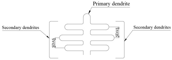
Figure 1.
SDAS definition: the distance between two secondary dendrites.

Table 1.
Magnification factor F and appropriate pixel per micrometer value.
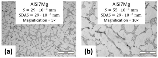
Figure 2.
The procedure of deriving different S values using different magnifications on the microscope: (a) 5× magnification image; (b) 10× magnification image. The scale bar corresponds to S value.
Table 2.
Images count per different material and different magnification.
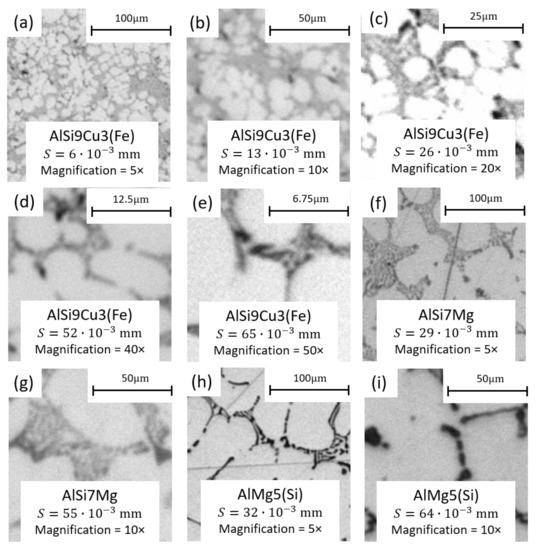
Figure 3.
pixel images used for training, their derived S values and alloy.
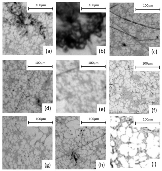
Figure 4.
Images of different types of defects used for the training: (a,b)—air and shrinkage porosity defects; (c,d)—scratches; (e)—blurred image; (c,f,g,i)—different brightness and contrast of the image; (g,h)—ECS (some images are purportedly of lower quality).
The image dataset for training consists of pixel images created from the original pixel images, as shown in Figure 5. The original image was first split into 70 images with a pixel resolution of , which were then resized to pixel. The S values and image count used for training, validation and testing are listed in Table 2. The training set, validation set and test set were split in the ratio 60:20:20. The data instances were evenly distributed in terms of S values.
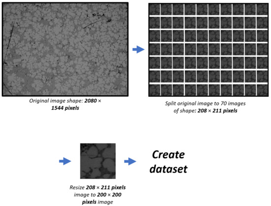
Figure 5.
Schematic representation of dataset generation: the original image was first split into 70 images with a pixel resolution of , which were then resized to pixel.
In an earlier approach [34], the images were preprocessed by the morphological transformation, Gaussian blur and Otsu’s threshold [35] to reduce the number of training parameters. The color scale of the image was reduced from an eight-bit three-channel depth (i.e., full RGB) to a one-bit color depth (e.g., black or white). Unfortunately, the approach requires manual tuning of the hyperparameters for each SDAS value, making it impractical. For the present study, grayscale images were used to achieve fully automatic detection of SDAS using DL to avoid any manual operation. Nevertheless, the training parameters were reduced by a factor of three by using only one color channel instead of three.
3.3. Overview of the CNN Model
Predictive model at hand is based on the CNN architecture. It is assumed that other ML approaches would exhibit inferior behavior and therefore they were not considered. In the present case, the CNN model is based on a basic feedforward (sequential) network. The model consists of three 2D convolutional layer blocks. Each convolutional filter is followed by a Rectified Linear Unit (ReLU) activation, batch normalization and a max-pooling layer. Filter sizes used were , and for the first, second and third convolutional layers, respectively. Zero-padding was applied evenly across both dimensions to compensate for edges. The convolutions were performed with stride 1. Each max-pooling filter was of size , and pooling was performed with stride 2. This resulted in the following intermediate activation maps: (input), (following the first convolutional block), (following the second convolutional block) and (following the third convolutional block). Activation of the final convolutional block was then flattened to create a meta-layer of 20,000 neurons, which was then followed by a fully-connected layer consisting of 64 neurons, followed by the ReLU activation function and batch normalization. Finally, this layer was then fully connected to the output layer, which contained a single linear neuron—because of the assumed regression operation. Thus, for a 2D input image of size , a single real value—S value is obtained. The Adam optimizer was used, using a learning rate of . The schematic CNN architecture is shown in Figure 6. The total number of parameters was 1,294,977. It was trained with the Keras library on an Intel® Core™ I7-4970 CPU running at 3.60 GHz using 8 parallel processing units. Training was completed in 5 h—for 30 epochs total. A batch size of 32 was used for the training.
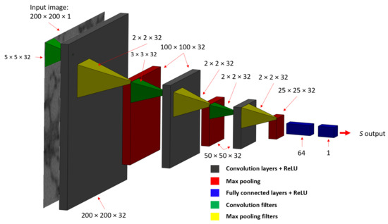
Figure 6.
The CNN architecture used for estimating SDAS directly from microstructure image patches.
4. Results and Discussion
The CNN model described in the previous section showed very good performance, having the score of on the test set. We performed an additional experiment to test the accuracy and practical usability of the model for possible industrial applications. The input image of pixel is taken as a reference and split into 70 images of pixel using the same approach as shown in Figure 5. The average result of 70 predictions is then captured while the prediction deviation and prediction error were also captured. We performed two mutually independent evaluation tests: one using materials that were used during the training, and another using materials that were not used during the training. It should be noted that individual images of both group of materials that were used for this test were not involved in the training, i.e., disjoint test subsets were used for both. The results are shown in Table 3 and Table 4, while the images used for the prediction task are shown in Figure 7 and Figure 8. S values were obtained using the same procedure as explained in the previous section.
Table 3.
Results of prediction for materials used during training.
Table 4.
Results of prediction for materials not used during training.
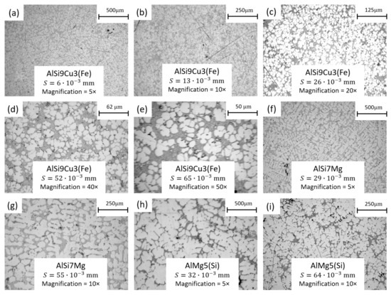
Figure 7.
Images of materials used during the training: The images were split into pixel images following the procedure in Figure 5 and used for the prediction task.
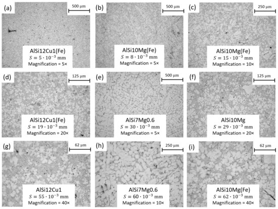
Figure 8.
Images of materials that were not used during the training: The images were split into pixel images following the procedure in Figure 5 and used for the prediction task.
The predicted results are very accurate for the trained materials. Average prediction deviation was evaluated for 10× magnification, giving only mm. Moreover, the maximum prediction deviation is mm, while every other prediction deviation is less than mm. In Table 3, it can be observed that a higher prediction deviation as well as a higher prediction error correlates with a smaller magnification. This could be directly attributed to the resolution of the images. At higher magnification, a dendrite is described with more pixels, so it is expected that the predicted results are more accurate. For example, the highest magnification of 50× results in an error of only 0.1 µm. Hopefully, SDAS smaller than mm is rarely seen in industrial applications. However, even assuming the highest deviation, such SDAS prediction model performances are quite acceptable for industry. A model with such performance could even be used to determine the SDAS distribution on a single microstructure image and/or polished cross-section sample.
The prediction error for the predicted results was also recorded. The average prediction error for the trained materials at 10× magnification is very low while the highest is . Again, the highest prediction errors were associated with the lowest resolution for all alloys considered. Increasing the number of pixels that depicts SDAS through higher magnification effectively eliminates the accuracy problem. At the highest magnifications, the errors were in the range of –, as can be seen in Table 3. It is therefore recommended to use a magnification of at least 10×.
In addition, prediction accuracy was also tested with materials that were not used during training (Table 4). The physical SDAS values of AlSi10Mg(Fe), AlSi12Cu1(Fe) and AlSi7Mg0.6 were mm, mm and mm, respectively. The results shown in Table 4 indicate that the predictions are less accurate than for the trained materials. The prediction error is also slightly higher, while the average prediction deviation is mm for highest magnifications. For the AlSi10Mg(Fe) alloy, the highest error of was obtained for 40× magnification, while errors close to were obtained for the other alloys. Note that a very high error (178%) was obtained for AlSi12Cu1(Fe) at low magnification, indicating that higher magnifications should again be preferred for the application of the CNN trained on other materials. This allows the error to be reduced to 3.5% for the 40× magnification, which is in the same range as when the CNN is applied to trained materials, cf. Table 3. For general analysis (e.g., to determine whether the component was cast in sand or in permanent mold, or for general determination of solidification rate), the model could be used successfully in the foundry industry, ensuring that magnification greater than 10× is used. As an example, even the deviation of the different measurement methods reported in [33] falls within the performance range of the model. The highest prediction deviation of mm was obtained for the alloy AlSi10Mg(Fe).
5. Conclusions
The present study confirms the hypothesis that SDAS can be determined directly from microstructure image data by the DL methodology. The model shows excellent performance on the materials used in the training, provided that the highest possible magnification is used. On the other hand, the model performs slightly worse for the materials not used in training. However, both variants could be used in any type of industry depending on the model accuracy. A model for materials used during training could even be used to determine the distribution of SDAS on a single microstructure image and/or polished cross-section sample. Furthermore, the model could still be applied for materials not used during training, although some caution should be exercised. Thus, from the discussion shown, it appears that the technique based on DL can predict SDAS with a high degree of certainty.
Since manual tuning of hyperparameter values is avoided in the present study, such an approach could be fully automated. Furthermore, this approach now has a potential application as part of Industry 4.0 for the automotive or other sector. Additionally, the methods of DL could also have a potential application for automated prediction of mechanical properties from an image of the microstructure. However, for this type of task, the link between SDAS and material properties should be part of the analysis.
Supplementary Materials
The following are available online at https://www.mdpi.com/article/10.3390/met11050756/s1, Figure S1: Images used for training (Figure 3, full resolution). Figure S2: Images of different types of defects used for the training (Figure 4, full resolution).
Author Contributions
Conceptualization, methodology, software, validation, investigation, writing—review and editing: F.N., I.Š. and M.Č. All the authors contributed equally to this work. All authors have read and agreed to the published version of the manuscript.
Funding
This research received no external funding.
Data Availability Statement
Data required to reproduce these findings are available for download from: http://dx.doi.org/10.17632/jkp57kbzxn.1, accessed on 31 March 2021. The following dataset consists of figures which are used during the training of the convolutional neural network as well as saved weights of the convolutional neural network after the training.
Acknowledgments
This work has been partially supported by the University of Rijeka under the project number uniri-tehnic-18-37. Polished samples were purchased from the University of Ljubljana: Faculty of Natural Sciences and Engineering. Additional samples were donated by TC Livarstvo d.o.o, and CIMOS d.d. Automotive Industry. This support is gratefully acknowledged.
Conflicts of Interest
The authors declare no conflict of interest.
References
- Vandersluis, E.; Ravindran, C. Relationships between solidification parameters in A319 aluminum alloy. J. Mater. Eng. Perform. 2018, 27, 1109–1121. [Google Scholar] [CrossRef]
- Vandersluis, E.; Ravindran, C. Influence of solidification rate on the microstructure, mechanical properties, and thermal conductivity of cast A319 Al alloy. J. Mater. Sci. 2019, 54, 4325–4339. [Google Scholar] [CrossRef]
- Djurdjevič, M.; Grzinčič, M. The effect of major alloying elements on the size of the secondary dendrite arm spacing in the as-cast Al-Si-Cu alloys. Arch. Foundry Eng. 2012, 12, 19–24. [Google Scholar] [CrossRef]
- Brusethaug, S.; Langsrud, Y. Aluminum properties, a model for calculating mechanical properties in AlSiMgFe-foundry alloys. Metall. Sci. Tecnol. 2000, 18, 3–7. [Google Scholar]
- Shabestari, S.; Shahri, F. Influence of modification, solidification conditions and heat treatment on the microstructure and mechanical properties of A356 aluminum alloy. J. Mater. Sci. 2004, 39, 2023–2032. [Google Scholar] [CrossRef]
- Kabir, M.S.; Ashrafi, A.; Minhaj, T.I.; Islam, M.M. Effect of foundry variables on the casting quality of as-cast LM25 aluminium alloy. Int. J. Eng. Adv. Technol. 2014, 3, 115–120. [Google Scholar]
- Seifeddine, S.; Wessen, M.; Svensson, I. Use of simulation to predict microstructure and mechanical properties in an as-cast aluminium cylinder head comparison-with experiments. Metall. Sci. Tecnol. 2006, 24, 7. [Google Scholar]
- Morri, A. Empirical models of mechanical behaviour of Al-Si-Mg cast alloys for high performance engine applications. Metall. Sci. Technol. 2010, 28, 25–32. [Google Scholar]
- Grosselle, F.; Timelli, G.; Bonollo, F.; Della Corte, E. Correlation between microstructure and mechanical properties of Al-Si cast alloys. La Metallurgia Italiana 2009, 27, 25–32. [Google Scholar]
- Qi, M.; Li, J.; Kang, Y. Correlation between segregation behavior and wall thickness in a rheological high pressure die-casting AC46000 aluminum alloy. J. Mater. Res. Technol. 2019, 8, 3565–3579. [Google Scholar] [CrossRef]
- Singh, S.; Bhadeshia, H.; MacKay, D.; Carey, H.; Martin, I. Neural network analysis of steel plate processing. Ironmak. Steelmak. 1998, 25, 355–365. [Google Scholar]
- Hancheng, Q.; Bocai, X.; Shangzheng, L.; Fagen, W. Fuzzy neural network modeling of material properties. J. Mater. Process. Technol. 2002, 122, 196–200. [Google Scholar] [CrossRef]
- Agrawal, A.; Deshpande, P.D.; Cecen, A.; Basavarsu, G.P.; Choudhary, A.N.; Kalidindi, S.R. Exploration of data science techniques to predict fatigue strength of steel from composition and processing parameters. Integr. Mater. Manuf. Innov. 2014, 3, 8. [Google Scholar] [CrossRef]
- Liu, R.; Kumar, A.; Chen, Z.; Agrawal, A.; Sundararaghavan, V.; Choudhary, A. A predictive machine learning approach for microstructure optimization and materials design. Sci. Rep. 2015, 5, 11551. [Google Scholar] [CrossRef]
- Yang, X.W.; Zhu, J.C.; Nong, Z.S.; Dong, H.; Lai, Z.H.; Ying, L.; Liu, F.W. Prediction of mechanical properties of A357 alloy using artificial neural network. Trans. Nonferrous Met. Soc. China 2013, 23, 788–795. [Google Scholar] [CrossRef]
- Santos, I.; Nieves, J.; Penya, Y.K.; Bringas, P.G. Machine-learning-based mechanical properties prediction in foundry production. In Proceedings of the 2009 ICCAS-SICE, Fukuoka City, Japan, 18–21 August 2009; pp. 4536–4541. [Google Scholar]
- Liao, H.; Zhao, B.; Suo, X.; Wang, Q. Prediction models for macro shrinkage of aluminum alloys based on machine learning algorithms. Mater. Today Commun. 2019, 21, 100715. [Google Scholar] [CrossRef]
- Agrawal, A.; Choudhary, A. Deep materials informatics: Applications of deep learning in materials science. MRS Commun. 2019, 9, 779–792. [Google Scholar] [CrossRef]
- Herriott, C.; Spear, A.D. Predicting microstructure-dependent mechanical properties in additively manufactured metals with machine-and deep-learning methods. Comput. Mater. Sci. 2020, 175, 109599. [Google Scholar] [CrossRef]
- Ferguson, M.K.; Ronay, A.; Lee, Y.T.T.; Law, K.H. Detection and segmentation of manufacturing defects with convolutional neural networks and transfer learning. Smart Sustain. Manuf. Syst. 2018, 2, 1–42. [Google Scholar] [CrossRef]
- Hanumantha Rao, D.; Tagore, G.; Ranga Janardhana, G. Evolution of Artificial Neural Network (ANN) model for predicting secondary dendrite arm spacing in aluminium alloy casting. J. Braz. Soc. Mech. Sci. Eng. 2010, 32, 276–281. [Google Scholar] [CrossRef]
- Wei, J.; Chu, X.; Sun, X.Y.; Xu, K.; Deng, H.X.; Chen, J.; Wei, Z.; Lei, M. Machine learning in materials science. InfoMat 2019, 1, 338–358. [Google Scholar] [CrossRef]
- Azimi, S.M.; Britz, D.; Engstler, M.; Fritz, M.; Mücklich, F. Advanced steel microstructural classification by deep learning methods. Sci. Rep. 2018, 8, 2128. [Google Scholar] [CrossRef]
- Li, X.; Zhang, Y.; Zhao, H.; Burkhart, C.; Brinson, L.C.; Chen, W. A transfer learning approach for microstructure reconstruction and structure-property predictions. Sci. Rep. 2018, 8, 13461. [Google Scholar] [CrossRef]
- Mery, D. Aluminum Casting Inspection Using Deep Learning: A Method Based on Convolutional Neural Networks. J. Nondestruct. Eval. 2020, 39, 12. [Google Scholar] [CrossRef]
- DeCost, B.L.; Lei, B.; Francis, T.; Holm, E.A. High throughput quantitative metallography for complex microstructures using deep learning: A case study in ultrahigh carbon steel. arXiv 2018, arXiv:1805.08693. [Google Scholar] [CrossRef]
- Chowdhury, A.; Kautz, E.; Yener, B.; Lewis, D. Image driven machine learning methods for microstructure recognition. Comput. Mater. Sci. 2016, 123, 176–187. [Google Scholar] [CrossRef]
- Exl, L.; Fischbacher, J.; Kovacs, A.; Oezelt, H.; Gusenbauer, M.; Yokota, K.; Shoji, T.; Hrkac, G.; Schrefl, T. Magnetic microstructure machine learning analysis. J. Phys. Mater. 2018, 2, 014001. [Google Scholar] [CrossRef]
- Yucel, B.; Yucel, S.; Ray, A.; Duprez, L.; Kalidindi, S.R. Mining the Correlations Between Optical Micrographs and Mechanical Properties of Cold-Rolled HSLA Steels Using Machine Learning Approaches. Integr. Mater. Manuf. Innov. 2020, 9, 240–256. [Google Scholar] [CrossRef]
- Pokuri, B.S.S.; Ghosal, S.; Kokate, A.; Sarkar, S.; Ganapathysubramanian, B. Interpretable deep learning for guided microstructure-property explorations in photovoltaics. NPJ Comput. Mater. 2019, 5, 95. [Google Scholar] [CrossRef]
- DeCost, B.L.; Holm, E.A. A computer vision approach for automated analysis and classification of microstructural image data. Comput. Mater. Sci. 2015, 110, 126–133. [Google Scholar] [CrossRef]
- DIN EN 1706: Aluminium und Aluminiumlegierungen-Gussstücke-Chemische Zusammensetzung und mechanische Eigenschaften; Beuth: Berlin, Germany, 1998.
- Vandersluis, E.; Ravindran, C. Comparison of measurement methods for secondary dendrite arm spacing. Metallogr. Microstruct. Anal. 2017, 6, 89–94. [Google Scholar] [CrossRef]
- Nikolic, F.; Štajduhar, I.; Čanađija, M. Aluminum microstructure inspection using deep learning: A convolutional neural network approach toward secondary dendrite arm spacing determination. In 4th Edition of My First Conference; University of Rijeka, Faculty of Engineering: Rijeka, Croatia, 2020. [Google Scholar]
- Alexander Mordvintsev, A.K.R. Image Processing in OpenCV. 2013. Available online: https://opencv-python-tutroals.readthedocs.io/en/latest/py_tutorials/py_imgproc/py_table_of_contents_imgproc/py_table_of_contents_imgproc.html (accessed on 5 September 2020).


Publisher’s Note: MDPI stays neutral with regard to jurisdictional claims in published maps and institutional affiliations. |
© 2021 by the authors. Licensee MDPI, Basel, Switzerland. This article is an open access article distributed under the terms and conditions of the Creative Commons Attribution (CC BY) license (https://creativecommons.org/licenses/by/4.0/).