Evidence and Credibility: Full Bayesian Significance Test for Precise Hypotheses

Abstract

A Bayesian measure of evidence for precise hypotheses is presented. The intention is to give a Bayesian alternative to significance tests or, equivalently, to p-values. In fact, a set is defined in the parameter space and the posterior probability, its credibility, is evaluated. This set is the “Highest Posterior Density Region” that is “tangent” to the set that defines the null hypothesis. Our measure of evidence is the complement of the credibility of the “tangent” region.

1. Introduction

The objective of this paper is to provide a coherent Bayesian measure of evidence for precise null hypotheses. Significance tests [1] are regarded as procedures for measuring the consistency of data with a null hypothesis by the calculation of a p-value (tail area under the null hypothesis). [2] and [3] consider the p-value as a measure of evidence of the null hypothesis and present alternative Bayesian measures of evidence, the Bayes Factor and the posterior probability of the null hypothesis. As pointed out in [1], the first difficult to define the p-value is the way the sample space is ordered under the null hypothesis. [4] suggested a p-value that always regards the alternative hypothesis. To each of these measures of evidence one could find a great number of counter arguments. The most important argument against Bayesian test for precise hypothesis is presented by [5]. Arguments against the classical p-value are full in the literature. The book by [6] and its review by [7] present interesting and relevant arguments to the statisticians start to thing about new methods of measuring evidence. In a more philosophical terms, [8] discuss, in a great detail, the concept of evidence. The method we suggest in the present paper has simple arguments and a geometric interpretation. It can be easily implemented using modern numerical optimization and integration techniques. To illustrate the method we apply it to standard statistical problems with multinomial distributions. Also, to show its broad spectrum, we consider the case of comparing two gamma distributions, which has no simple solution with standard procedures. It is not a situation that appears in regular textbooks. These examples will make clear how the method should be used in most situations. The method is “Full” Bayesian and consists in the analysis of credible sets. By Full we mean that one needs only to use the posterior distribution without the need for any adhockery, a term used by [8].

2. The Evidence Calculus

Consider the random variable D that, when observed, produces the data d. The statistical space is represented by the triplet $(\Xi ,\Delta ,\Theta )$ where $\Xi$ is the sample space, the set of possible values of d, $\Delta$ is the family of measurable subsets of $\Xi$ and $\Theta$ is the parameter space. We define now a prior model $(\Theta ,B,{\pi }_d)$, which is a probability space defined over $\Theta$. Note that this model has to be consistent, so that $\mathrm{Pr}(A|\theta )$ turns out to be well defined. As usual after observing data d, we obtain the posterior probability model $(\Theta ,B,{\pi }_d)$, where ${\pi }_d$ is the conditional probability measure on $B$ given the observed sample point, $d$. In this paper we restrict ourselves to the case where the function ${\pi }_d$ has a probability density function.

To define our procedure we should concentrate only on the posterior probability space $(\Theta ,B,{\pi }_d)$. First we will define $T_{\varphi }$ as the subset of the parameter space where the posterior density is greater than $\varphi$.

$$T_{\varphi }=\left\{\theta \in \Theta |f(\theta )\varphi \right\}$$

The credibility of $T_{\varphi }$ is its posterior probability,

$$\kappa ={\displaystyle {\int }_{ T_{\varphi }}f(\theta |d)d\theta } = {\displaystyle {\int }_{ \Theta }{f}_{\varphi }(\theta |d)d}\theta$$

where $f_{\varphi }(x)=f(x)$ if $f(x)\varphi$ and zero otherwise.

Now, we define f^* as the maximum of the posterior density over the null hypothesis, attained at the argument $\theta *$,

$$\theta *\in \arg \underset{\theta \in {\Theta }_0}{\max }f(\theta ), f*=f(\theta *)$$

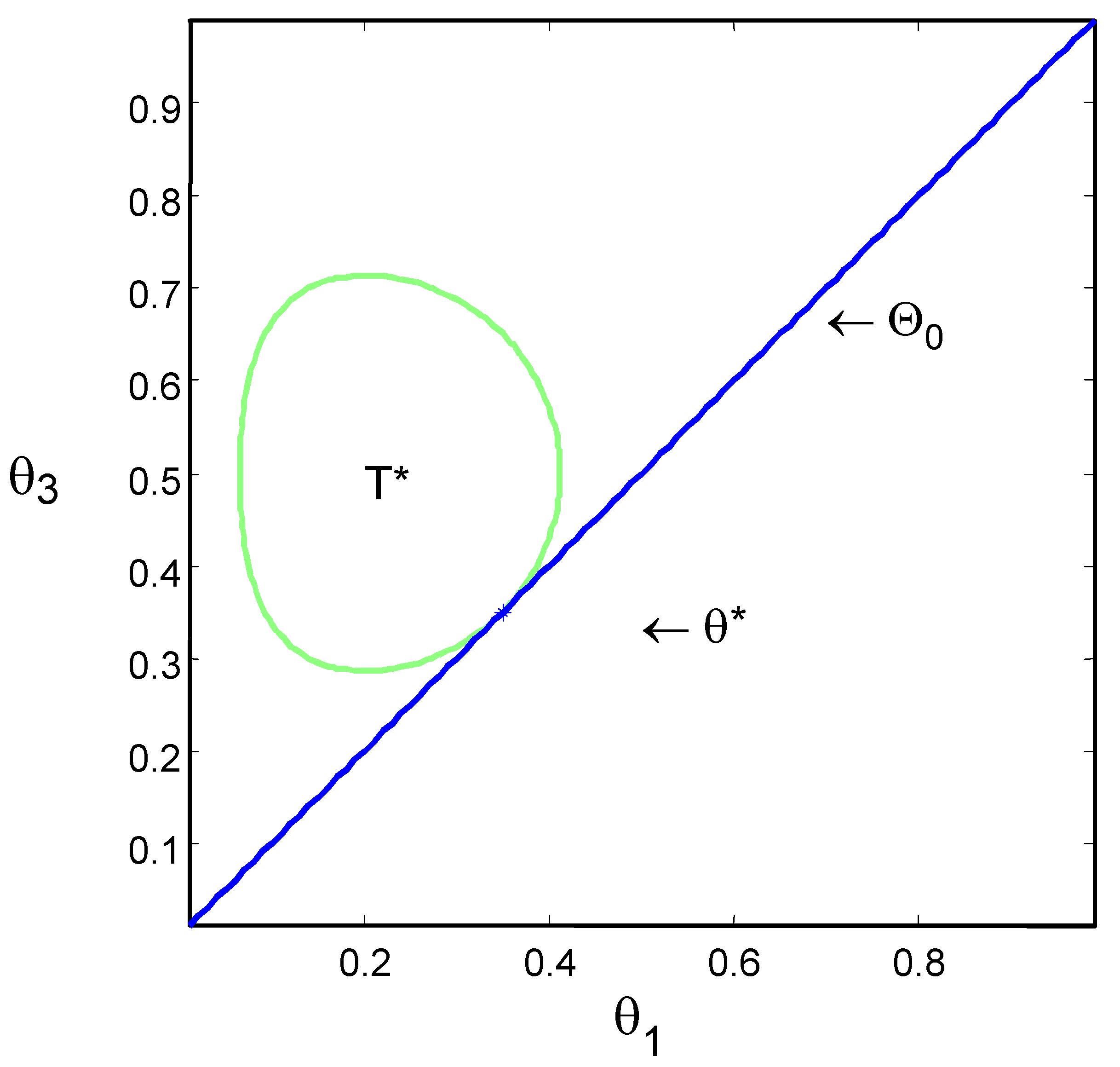
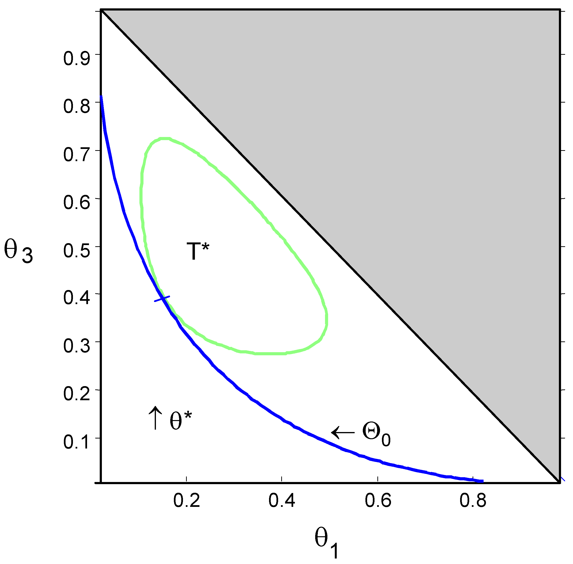
and define $T*=T_{f*}$ as the set “tangent” to the null hypothesis, H, whose credibility is $\kappa *$. Figure 1 and Figure 2 show the null hypothesis and the contour of set T^* for Examples 2 and 3 of Section 4.

The measure of evidence we propose in this article is the complement of the probability of the set T^*. That is, the evidence of the null hypothesis is

$$Ev(H)=1-\kappa *\text{ or }1-{\pi }_d(T*).$$

If the probability of the set T^* is “large”, it means that the null set is in a region of low probability and the evidence in the data is against the null hypothesis. On the other hand, if the probability of T^* is “small”, then the null set is in a region of high probability and the evidence in the data is in favor of the null hypothesis.

Although the definition of evidence above is quite general, it was created with the objective of testing precise hypotheses. That is, a null hypothesis for which the dimension is smaller than that of the parameter space, i.e. $\dim ({\Theta }_0)\dim (\Theta )$.

3. Numerical Computation

In this paper the parameter space, $\Theta$, is always a subset of Rⁿ, and the hypothesis is defined as a further restricted subset ${\Theta }_0\subset \Theta \subseteq R^n$. Usually, ${\Theta }_0$is defined by vector valued inequality and equality constraints:

$${\Theta }_0=\left\{\theta \in \Theta |g(\theta )\le 0 \wedge h(\theta )=0\right\}.$$

Since we are working with precise hypotheses, we have at least one equality constraint, hence $\dim ({\Theta }_0)\dim (\Theta )$. Let $f(\theta )$ be the probability density function for the measure ${\pi }_d$, i.e.,

$${\pi }_d(b)={\displaystyle {\int }_{ b}f(\theta )d\theta }.$$

The computation of the evidence measure defined in the last section is performed in two steps, a numerical optimization step, and a numerical integration step. The numerical optimization step consists of finding an argument $\theta *$ that maximizes the posterior density $f(\theta )$under the null hypothesis. The numerical integration step consists of integrating the posterior density over the region where it is greater than $f(\theta *)$. That is,

• Numerical Optimization step:

  $$\theta *\in \arg \underset{\theta \in {\Theta }_0}{\max }f(\theta ), \varphi =f*=f(\theta *)$$
• Numerical Integration step:

$$\kappa *={\displaystyle {\int }_{ \Theta }{f}_{\varphi }(\theta |d)d}\theta$$

where $f_{\varphi }(x)=f(x)$ if $f(x)\varphi$ and zero otherwise.

Efficient computational algorithms are available for local and global optimization as well as for numerical integration in [9], [10], [11], [12], [13], and [14]. Computer codes for several such algorithms can be found at software libraries as NAG and ACM, or at internet sites as www.ornl.org.

We notice that the method used to obtain T^* and to calculate $\kappa *$ can be used under general conditions. Our purpose, however, is to discuss precise hypothesis testing, under absolute continuity of the posterior probability model, the case for which most solutions presented in the literature are controversial.

4. Examples

In the sequel we will discuss five examples with increasing computational difficulty. The first four are about the Multinomial model. The first example presents the test for a specific success rate in the standard binomial model, and the second is about the equality of two such rates. For these two examples the null hypotheses are linear restrictions of the original parameter spaces. The third example introduces the Hardy-Weinberg equilibrium hypothesis in a trinomial distribution. In this case the hypothesis is quadratic.

Forth example considers the test of independence of two events in a $2\times 2$ contingency table. In this case the parameter space has dimension three, and the null hypothesis, which is not linear, defines a set of dimension two.

Finally, the last example presents two parametric comparisons for two gamma distributions. Although straightforward in our paradigm, it is not presented by standard statistical textbooks. We believe that, the reason for this gap in the literature is the non-existence of closed analytical forms for the test. In order to be able to fairly compare our evidence measure with standard tests, like Chi-square tail (pV), Bayes Factor (BF), and Posterior-Probability (PP), we always assume a uniform prior distribution. In these examples the likelihood has finite integral over the parameter space. Hence we have posterior density functions that are proportional to the respective likelihood functions. In order to achieve better numerical stability we optimize a function proportional to the log-likelihood, $L(\theta )$, and make explicit use of its first and second derivatives (gradient and Jacobian).

For the 4 examples concerning multinomial distributions we present the following figures (Table 1, Table 2, and Table 3):

• Our measure of evidence, Ev, for each d;
• the p-value, pV obtained by the ${\chi }^2$ test; that is, the tail area;
• the Bayes Factor,

  $$BF=\frac{\mathrm{Pr}\left\{{\Theta }_0\right\}\mathrm{Pr}\left\{d|{\Theta }_0\right\}}{\left(1-\mathrm{Pr}\left\{{\Theta }_0\right\}\right) \mathrm{Pr}\left\{d|\Theta -{\Theta }_0\right\}}; \mathrm{and}$$
• the posterior probability of H,

  $$PP=\mathrm{Pr}\left\{{\Theta }_0|d\right\}={\left\{1+{(BF)}^{-1}\right\}}^{-1}.$$

For the definition of the Bayes Factor and properties we refer to [8] and [15].

4.1. Success rate in standard binomial model

This is a standard example about testing that a proportion, $\theta$, is equal to a specific value, p. Consider the random variable, D being binomial with parameter $\theta$ and sample size n. Here we consider $n=20$ trials, $p=0.5$ and d is the observed success number. The parameter space is the unit interval $\Theta =\left\{0\le \theta \le 1\right\}$. The null hypothesis is defined as $H:\theta =p$. For all possible values of d, Table 1 presents the figures to compare our measure with the standard ones. To compute the Bayes Factor, we consider a priori $\mathrm{Pr}\left\{H\right\}=\mathrm{Pr}\left\{\theta =p\right\}=0.5$ and a uniform density for $\theta$ under the “alternative” hypothesis, $A:\theta \ne p$. That is,

$$BF=(n+1) \left(\begin{array}{c}n\\ d\end{array}\right) p^d{(1-p)}^{n-d}.$$

Table 1. Standard binomial model.

d	Ev	PV	BF	PP
0	0.00	0.00	0.00	0.00
1	0.00	0.00	0.00	0.00
2	0.00	0.00	0.00	0.00
3	0.00	0.00	0.02	0.02
4	0.01	0.01	0.10	0.09
5	0.02	0.03	0.31	0.24
6	0.06	0.07	0.78	0.44
7	0.16	0.18	1.55	0.61
8	0.35	0.37	2.52	0.72
9	0.64	0.65	3.36	0.77
10	1.00	1.00	3.70	0.79

Table 1. Standard binomial model.

d	Ev	PV	BF	PP
0	0.00	0.00	0.00	0.00
1	0.00	0.00	0.00	0.00
2	0.00	0.00	0.00	0.00
3	0.00	0.00	0.02	0.02
4	0.01	0.01	0.10	0.09
5	0.02	0.03	0.31	0.24
6	0.06	0.07	0.78	0.44
7	0.16	0.18	1.55	0.61
8	0.35	0.37	2.52	0.72
9	0.64	0.65	3.36	0.77
10	1.00	1.00	3.70	0.79

4.2. Homogeneity test in 2× 2 contingency table

This model is useful in many applications, like comparison of two communities with relation to a disease incidence, consumer behavior, electoral preference, etc. Two samples are taken from two binomial populations, and the objective is to test whether the success ratios are equal. Let x and y be the number of successes of two independent binomial experiments of sample sizes m and n, respectively. The posterior density for this multinomial model is

$$f(\theta |x,y,n,m) \propto {\theta }_1^x{\theta }_2^{n-x}{\theta }_3^y{\theta }_4^{m-y}.$$

The parameter space and the null hypothesis set are:

$$\Theta =\left\{0\le \theta \le 1 | {\theta }_1+{\theta }_2=1 \wedge {\theta }_3+{\theta }_4=1\right\}$$

$${\Theta }_0=\left\{\theta \in \Theta |{\theta }_1={\theta }_3\right\}.$$

The Bayes Factor considering a priori $\mathrm{Pr}\left\{H\right\} = \mathrm{Pr}\left\{{\theta }_1={\theta }_3\right\} = 0.5$ and uniform densities over ${\theta }_0$ and $\theta -{\theta }_0$ is given in the equation below. See [16] and [17] for details and discussion about properties.

$$BF = \frac{\left(\begin{array}{c}m\\ x\end{array}\right) \left(\begin{array}{c}n\\ y\end{array}\right)}{\left(\begin{array}{c}m+n\\ x+y\end{array}\right)} \frac{(m+1) (n+1)}{m+n+1}$$

Left side of Table 2 presents figures to compare Ev(d) with the other standard measures for $m=n=20$. Figure 1 presents H and T* for $x=10$ and $y=4$ with $n=m=20$.

Table 2. Tests of homogeneity and Hardy-Weinberg equilibrium.

Homogeneity						Hardy-Weinberg
x	y	Ev	pV	BF	PP	x1	x3	Ev	pV	BF	PP
5	0	0.05	0.02	0.25	0.20	1	2	0.01	0.00	0.01	0.01
5	1	0.18	0.08	0.87	0.46	1	3	0.01	0.01	0.04	0.04
5	2	0.43	0.21	1.70	0.63	1	4	0.04	0.02	0.11	0.10
5	3	0.71	0.43	2.47	0.71	1	5	0.09	0.04	0.25	0.20
5	4	0.93	0.71	2.95	0.75	1	6	0.18	0.08	0.46	0.32
5	5	1.00	1.00	3.05	0.75	1	7	0.31	0.15	0.77	0.44
5	6	0.94	0.72	2.80	0.74	1	8	0.48	0.26	1.16	0.54
5	7	0.77	0.49	2.31	0.70	1	9	0.66	0.39	1.59	0.61
5	8	0.58	0.31	1.75	0.64	1	10	0.83	0.57	2.00	0.67
5	9	0.39	0.18	1.21	0.55	1	11	0.95	0.77	2.34	0.70
5	10	0.24	0.10	0.77	0.43	1	12	1.00	0.99	2.55	0.72
10	0	0.00	0.00	0.00	0.00	1	13	0.96	0.78	2.57	0.72
10	1	0.00	0.00	0.02	0.02	1	14	0.84	0.55	2.39	0.71
10	2	0.01	0.01	0.07	0.06	1	15	0.66	0.33	2.05	0.67
10	3	0.05	0.02	0.19	0.16	1	16	0.47	0.16	1.58	0.61
10	4	0.12	0.05	0.41	0.29	1	17	0.27	0.05	1.06	0.51
10	5	0.24	0.10	0.77	0.43	1	18	0.12	0.00	0.58	0.37
10	6	0.41	0.20	1.23	0.55	5	0	0.02	0.01	0.05	0.05
10	7	0.61	0.34	1.74	0.63	5	1	0.09	0.04	0.25	0.20
10	8	0.81	0.53	2.21	0.69	5	2	0.29	0.14	0.60	0.38
10	9	0.95	0.75	2.54	0.72	5	3	0.61	0.34	1.00	0.50
10	10	1.00	1.00	2.66	0.73	5	4	0.89	0.65	1.29	0.56
12	0	0.00	0.00	0.00	0.00	5	5	1.00	1.00	1.34	0.57
12	1	0.00	0.00	0.00	0.00	5	6	0.90	0.66	1.18	0.54
12	2	0.00	0.00	0.01	0.01	5	7	0.66	0.39	0.89	0.47
12	3	0.01	0.00	0.04	0.04	5	8	0.40	0.20	0.58	0.37
12	4	0.03	0.01	0.10	0.09	5	9	0.21	0.09	0.32	0.24
12	5	0.07	0.03	0.24	0.19	5	10	0.09	0.04	0.16	0.13
12	6	0.14	0.06	0.46	0.32	9	0	0.21	0.09	0.73	0.42
12	7	0.26	0.11	0.80	0.44	9	1	0.66	0.39	1.59	0.61
12	8	0.42	0.21	1.24	0.55	9	2	0.99	0.91	1.77	0.64
12	9	0.62	0.34	1.73	0.63	9	3	0.86	0.59	1.33	0.57
12	10	0.81	0.53	2.21	0.69	9	4	0.49	0.26	0.74	0.43
						9	5	0.21	0.09	0.32	0.24
						9	6	0.06	0.03	0.11	0.10
						9	7	0.01	0.01	0.03	0.03

Table 2. Tests of homogeneity and Hardy-Weinberg equilibrium.

Homogeneity						Hardy-Weinberg
x	y	Ev	pV	BF	PP	x1	x3	Ev	pV	BF	PP
5	0	0.05	0.02	0.25	0.20	1	2	0.01	0.00	0.01	0.01
5	1	0.18	0.08	0.87	0.46	1	3	0.01	0.01	0.04	0.04
5	2	0.43	0.21	1.70	0.63	1	4	0.04	0.02	0.11	0.10
5	3	0.71	0.43	2.47	0.71	1	5	0.09	0.04	0.25	0.20
5	4	0.93	0.71	2.95	0.75	1	6	0.18	0.08	0.46	0.32
5	5	1.00	1.00	3.05	0.75	1	7	0.31	0.15	0.77	0.44
5	6	0.94	0.72	2.80	0.74	1	8	0.48	0.26	1.16	0.54
5	7	0.77	0.49	2.31	0.70	1	9	0.66	0.39	1.59	0.61
5	8	0.58	0.31	1.75	0.64	1	10	0.83	0.57	2.00	0.67
5	9	0.39	0.18	1.21	0.55	1	11	0.95	0.77	2.34	0.70
5	10	0.24	0.10	0.77	0.43	1	12	1.00	0.99	2.55	0.72
10	0	0.00	0.00	0.00	0.00	1	13	0.96	0.78	2.57	0.72
10	1	0.00	0.00	0.02	0.02	1	14	0.84	0.55	2.39	0.71
10	2	0.01	0.01	0.07	0.06	1	15	0.66	0.33	2.05	0.67
10	3	0.05	0.02	0.19	0.16	1	16	0.47	0.16	1.58	0.61
10	4	0.12	0.05	0.41	0.29	1	17	0.27	0.05	1.06	0.51
10	5	0.24	0.10	0.77	0.43	1	18	0.12	0.00	0.58	0.37
10	6	0.41	0.20	1.23	0.55	5	0	0.02	0.01	0.05	0.05
10	7	0.61	0.34	1.74	0.63	5	1	0.09	0.04	0.25	0.20
10	8	0.81	0.53	2.21	0.69	5	2	0.29	0.14	0.60	0.38
10	9	0.95	0.75	2.54	0.72	5	3	0.61	0.34	1.00	0.50
10	10	1.00	1.00	2.66	0.73	5	4	0.89	0.65	1.29	0.56
12	0	0.00	0.00	0.00	0.00	5	5	1.00	1.00	1.34	0.57
12	1	0.00	0.00	0.00	0.00	5	6	0.90	0.66	1.18	0.54
12	2	0.00	0.00	0.01	0.01	5	7	0.66	0.39	0.89	0.47
12	3	0.01	0.00	0.04	0.04	5	8	0.40	0.20	0.58	0.37
12	4	0.03	0.01	0.10	0.09	5	9	0.21	0.09	0.32	0.24
12	5	0.07	0.03	0.24	0.19	5	10	0.09	0.04	0.16	0.13
12	6	0.14	0.06	0.46	0.32	9	0	0.21	0.09	0.73	0.42
12	7	0.26	0.11	0.80	0.44	9	1	0.66	0.39	1.59	0.61
12	8	0.42	0.21	1.24	0.55	9	2	0.99	0.91	1.77	0.64
12	9	0.62	0.34	1.73	0.63	9	3	0.86	0.59	1.33	0.57
12	10	0.81	0.53	2.21	0.69	9	4	0.49	0.26	0.74	0.43
						9	5	0.21	0.09	0.32	0.24
						9	6	0.06	0.03	0.11	0.10
						9	7	0.01	0.01	0.03	0.03

Figure 1. Homogeneity test with $x=10$, $y=4$ and $n=m=20$.

Figure 1. Homogeneity test with $x=10$, $y=4$ and $n=m=20$.

4.3. Hardy-Weinberg equilibrium law

In this biological application there is a sample of n individuals, where x₁ and x₃ are the two homozigote sample counts and $x_2=n-x_1-x_3$ is hetherozigote sample count. $\theta =\left[{\theta }_1,{\theta }_2,{\theta }_3\right]$ is the parameter vector. The posterior density for this trinomial model is

$$f(\theta |x) \propto {\theta }_1^{x_1}{\theta }_2^{x_2}{\theta }_3^{x_3}$$

The parameter space and the null hypothesis set are:

$$\Theta =\left\{\theta \ge 0 | {\theta }_1+{\theta }_2+{\theta }_3=1\right\}$$

$${\Theta }_0=\left\{\theta \in \Theta | {\theta }_3={\left(1 - \sqrt{{\theta }_1}\right)}^2\right\}$$

The problem of testing the Hardy-Weinberg equilibrium law using the Bayes Factor is discussed in detail by [18] and [19].

The Bayes Factor considering uniform priors over ${\theta }_0$ and $\theta -{\theta }_0$ is given by the following expression:

$$BF = \frac{(n+2)! t! (2n-t)! 2^{x_2}}{(2n+1)! x_1! x_2! x_3!} \left[5/6 - \frac{2 (t+1) (2n-t+1)}{(2n+2) (2n+3)}\right]$$

Here $t=2x_1+x_2$ is a sufficient statistic under H. This means that the likelihood under H depends on data d only through t.

Right side of Table 2 presents figures to compare Ev(d) with the other standard measures for $n=20$. Figure 2 presents H and T^* for $x_1=5$, $x_3=10$ and $n=20$.

4.4. Independence test in a 2× 2 contingency table

Suppose that laboratory test is used to help in the diagnostic of a disease. It should be interesting to check if the test results are really related to the health conditions of a patient. A patient chosen from a clinic is classified as one of the four states of the set

$$\left\{(h,t)|h,t=0\text{ or }1\right\}$$

in such a way that h is the indicator of the occurrence or not of the disease and t is the indicator for the laboratory test being positive or negative. For a sample of size n we record $(x_{00},x_{01},x_{10},x_{11})$, the vector whose components are the sample frequency of each the possibilities of (t,h). The parameter space is the simplex

$$\Theta =\left\{\left({\theta }_{00},{\theta }_{01},{\theta }_{10},{\theta }_{11}\right) | {\theta }_{ij}\ge 0 \wedge {\displaystyle \sum _{i,j}{\theta }_{ij}}=1\right\}$$

and the null hypothesis, h and t are independent, is defined by

$${\Theta }_0=\left\{\theta \in \Theta | {\theta }_{00}={\theta }_{0•}{\theta }_{•0}, {\theta }_{0•}={\theta }_{00}+{\theta }_{01}, {\theta }_{•0}={\theta }_{00}+{\theta }_{10}\right\}$$

Figure 2. Hardy-Weinberg test with $x_1=5$, $x_3=10$ and $n=20$.

Figure 2. Hardy-Weinberg test with $x_1=5$, $x_3=10$ and $n=20$.

The Bayes Factor for this case is discussed by [17] and has the following expression:

$$BF = \frac{\left(\begin{array}{c}{x}_{0•}\\ x_{00}\end{array}\right) \left(\begin{array}{c}{x}_{1•}\\ x_{11}\end{array}\right)}{\left(\begin{array}{c}n\\ x_{•0}\end{array}\right)} \left\{\frac{(n+2) \left\{(n+3)-(n+2)\left[P(1-P)+Q(1-Q)\right]\right\}}{4(n+1)}\right\}$$

where $x_{i•}=x_{i0}+x_{i1}$, $x_{•j}=x_{0j}+x_{1j}$, $P=\frac{x_{0•}}{n+2}$ and $Q=\frac{x_{•0}}{n+2}$.

Table 3. Test of independence.

x00	x01	x10	x11	Ev	pV	BF	PP
12	6	95	35	0.96	0.57	4.73	0.83
48	25	9	10	0.54	0.14	1.04	0.51
96	50	18	20	0.24	0.04	0.50	0.33
18	5	39	30	0.29	0.06	0.50	0.33
36	10	78	60	0.06	0.01	0.11	0.10

Table 3. Test of independence.

x00	x01	x10	x11	Ev	pV	BF	PP
12	6	95	35	0.96	0.57	4.73	0.83
48	25	9	10	0.54	0.14	1.04	0.51
96	50	18	20	0.24	0.04	0.50	0.33
18	5	39	30	0.29	0.06	0.50	0.33
36	10	78	60	0.06	0.01	0.11	0.10

4.5. Comparison of two gamma distributions

This model may be used when comparing two survival distributions, for example, medical procedures and pharmacological efficiency, component reliability, financial market assets, etc. Let $\left[x_{1,1},x_{1,2},\dots ,x_{1,n_1}\right]$ and $\left[x_{2,1},x_{2,2},\dots ,x_{2,n_2}\right]$ be samples of two gamma distributed survival times. The sufficient statistic for the gamma distribution is the vector [n,s,p], i.e. the sample size, the observations sum and product. Let $\left[{\alpha }_1,{\beta }_1\right]$ and $\left[{\alpha }_2,{\beta }_2\right]$, all positive, be these gamma parameters. The likelihood function is:

$$f(n_1,{\alpha }_1,{\beta }_1,n_2,{\alpha }_2,{\beta }_2|data) \propto \frac{{\beta }_1^{{\alpha }_1{n}_1}}{\Gamma {({\alpha }_1)}^{n_1}} \frac{{\beta }_2^{{\alpha }_2{n}_2}}{\Gamma {({\alpha }_2)}^{n_2}} p_1^{{\alpha }_1-1} e^{-{\beta }_1{s}_1} p_2^{{\alpha }_2-1} e^{-{\beta }_2{s}_2}$$

This likelihood function is integrable on the parameter space. In order to allow comparisons with classical procedures, we will not consider any informative prior, i.e., the likelihood function will define by itself the posterior density.

Table 4 presents time to failure of coin comparators, a component of gaming machines, of two different brands. An entrepreneur was offered to replace brand 1 by the less expensive brand 2. The entrepreneur tested 10 coin comparators of each brand, and computed the sample means and standard deviations. The gamma distribution fits nicely this type of failure time, and was used to model the process. Denoting the gamma mean and standard deviation by $\mu =\alpha /\beta$ and $\sigma =\mu /\beta$, the first hypothesis to be considered is $H\text{'} : {\mu }_1={\mu }_2$. The high evidence of H', $Ev(H\text{'})=0.89$, corroborates the entrepreneur decision of changing its supplier. Note that the naive comparison of the sample means could be misleading. In the same direction, the low evidence of $H : {\mu }_1={\mu }_2 \wedge {\sigma }_1={\sigma }_2$, $Ev(H)=0.01$, indicates that the new brand should have smaller variation on the time to failure. The low evidence of H suggests that costs could be further diminished by na improved maintenance policy [20].

Table 4. Comparing two gamma distributions.

Brand 1 sample
39.27	31.72	12.33	27.67	56.66
28.32	53.72	29.71	23.76	33.55
mean1=33.67			std1=13.33
Brand 2 sample
28.32	53.72	29.71	23.76	33.55
24.07	33.79	33.10	26.93	27.23
mean2=29.25			std2=3.62
Evidence
$Ev(H\text{'})=0.89$			$Ev(H)=0.01$

Table 4. Comparing two gamma distributions.

Brand 1 sample
39.27	31.72	12.33	27.67	56.66
28.32	53.72	29.71	23.76	33.55
mean1=33.67			std1=13.33
Brand 2 sample
28.32	53.72	29.71	23.76	33.55
24.07	33.79	33.10	26.93	27.23
mean2=29.25			std2=3.62
Evidence
$Ev(H\text{'})=0.89$			$Ev(H)=0.01$

5. Final Remarks

The theory presented in this paper, grew out of the necessity of testing precise hypotheses made on the behavior of software controlled machines [21]. The hypotheses being tested are software requirements and specifications. The real machine software is not available, but the machine can be used for input-output black-box simulation. The authors had the responsibility of certifying whether gaming machines were working according to Brazilian law (requirements) and manufacturer's game description (specifications). Many of these requirements and specifications can be formulated as precise hypotheses on contingency tables, like the simple cases of Examples 1, 2 and 4. The standard methodologies, in our opinion, where not adequate to our needs and responsibilities. The classical p-value does not consider the alternative hypothesis that, in our case, is as important as the null hypothesis. Also the p-value is the measure of a tail in the sample space, whereas our concerns are formulated in the parameter space. On the other hand, we like the idea of measuring the significance of a precise hypothesis.

The Bayes factor is indeed formulated directly in the parameter space, but needs an ad hoc positive prior probability on the precise hypothesis. First we had no criterion to assess the required positive prior probability. Second we would be subject to Lindley's paradox, that would privilegiate the null hypothesis [5], [22].

The methodology of evidence calculus based on credible sets presented in this paper is computed in the parameter space, considers only the observed sample, has the significance flavor as in the p-value, and takes in to account the geometry of the null hypothesis as a surface (manifold) imbedded in the whole parameter space. Furthermore, this methodology takes into account only the location of the maximum likelihood under the null hypothesis, making it consistent with “benefit of the doubt” juridical principle. This methodology is also independent of the null hypothesis parametrization. This parametrization independence gives the methodology a geometric characterization, and is in sharp contrast with some well known procedures, like the Fisher exact test [23].

Recalling [6] in its Chapter 6, - “...recognizing that likelihoods are the proper means for representing statistical evidence simplifies and unifies statistical analysis.”- the measure Ev(H) defined in this paper is in accord with this Royall's principle.