Thermal Contact

Abstract

The concepts of temperature and entropy as applied in equilibrium thermodynamics do not easily generalize to nonequilibrium systems and there are transient systems where thermodynamics cannot apply. However, it is possible that nonequilibrium steady states may have a thermodynamics description. We explore the consequences of a particular microscopic thermostat-reservoir contact needed to both stabilize and measure the temperature of a system. One particular mechanical connection mechanism is considered in detail and a contact resistance is observed in the numerical simulations. We propose a microscopic mechanism to explain this effect for both equilibrium and nonequilibrium systems. These results emphasize the difficulty in identifying a microscopic expression for the thermodynamic temperature. It is evident that the kinetic temperature is not necessarily equal to the thermodynamic temperature, especially when used to define the local temperature.

1. Introduction

Entropy in nonequilibrium systems is a very difficult quantity. For an isolated equilibrium system the entropy is a maximum. However, if that system is connected to a reservoir and perturbed from equilibrium the system is said to produce entropy, but that entropy production is transferred to some reservoir or surroundings and the intrinsic entropy of the nonequilibrium system is lower than it is at equilibrium. Thus, when the perturbation is removed the relaxation is driven by an increase in the intrinsic entropy. Perhaps a more useful construct is to consider this entropy flow instead as a flow of energy through the system that maintains it in a steady state. This energy flow has been called the housekeeping heat [1] to distinguish it from other intrinsic heat flows. As well, following the axiomatic approach to equilibrium thermodynamics, the temperature is defined by the zeroth law, and the identification of the entropy follows as a consequence. It may well be better for nonequilibrium systems, to identify the temperature first and then look for a consistent nonequilibrium entropy.

From a macroscopic viewpoint the concept of temperature at equilibrium is well established by the zeroth law of thermodynamics. This involves the idea of bringing together two systems and allowing them to exchange energy. However, as soon as a microscopic treatment based on this idea is considered it is clear that a detailed microscopic mechanism that facilitates energy transfer is needed, and that involves both the structure of the systems and the details of the interaction at the boundary. One example where these microscopic details have been considered is the adiabatic piston separating two fluids [10]. This is somewhat beyond the zeroth law construction as we expect both thermal and mechanical equilibruim to be established. What these studies do show very clearly is that the piston becomes just like an extra particle. It has a temperature, and the fluctuations in this temperature allow heat to move from one fluid to the other. With two processes, heat flow and volume change, their rates become important, and typically mechanical equilibrium is established much faster than thermal equilibrium.

For systems away from equilibrium the status of the zeroth law is not clear. There have been a number of studies of possible nonequilibrium temperatures [2,3,4,5,6,7,8,9] but to date the question is not settled.

2. Concepts of Temperature

2.1. Macroscopic

The Zeroth Law of Thermodynamics proposed by Fowler and Planck was the last of the laws of thermodynamics to be formulated. It recognizes in an axiomatic way the fundamental importance of the concept of temperature and connects it with two of its properties - transitivity and measurability. The key ingredient is that the temperature is defined without reference to its conjugate variable - the entropy. If this were not possible then all arguments about thermodynamics would be circular.

The first concept of equilibrium statistical mechanics is the existence of an equilibrium state. Given two systems characterized by their values of pressure and volume, we propose that an equilibrium state exists. Following Callen [11] and Thompson [12] we associated with each pair of systems A and B a function $f(P_A,V_A,P_B,V_B)$ of the two states $(P_A,V_A)$ and $(P_B,V_B)$ such that if A and B are in equilibrium then

$$f(P_A,V_A,P_B,V_B)=0.$$

(1)

At this stage the assumption of the existence of an equilibrium state is the same as the assumption that the function f exists. The second concept is that if two systems A and B are in equilibrium and B is in equilibrium with C, then A must be in equilibrium with C. This implies that as well as equation (1) being satisfied for systems A and B, and B and C separately, we have

$$f(P_C,V_C,P_B,V_B)=0.$$

(2)

This is both a notion of transitivity and a statement about measurability. Physically, if system B is an ideal gas thermometer, then the fact that both A and C are both separately in equilibrium with B means that they both have the same temperature. Mathematically, given that equations (1) and (2) are satisfied, and the function f is continuous and has continuous partial derivatives, then the implicit function theorem states that

$$P_B=\Omega (P_A,V_A,V_B)=\Omega (P_C,V_C,V_B).$$

(3)

Now as B is a fixed system, $V_B$ is a constant, and we can ignore the $V_B$ dependence of Ω and define $\Omega (P_A,V_A)$ to be the empirical temperature of system A.

For systems that are away from equilibrium, but in steady non-transient states, we expect that the concept of a temperature may still apply. There are however, many situations where particular components of the system (different degrees of freedom) may have different values of the temperature, as energy constantly moves from one group of components (or degrees of freedom) of the system, to another, to maintain the steady state. This is observed in the molecular dynamics simulation of a nonequilibrium steady state Couette flow for molecular systems [13] where rotational and translational degrees of freedom have different kinetic temperatures. It is also usual for such a steady state to have different values of the pressure in different directions, so the diagonal elements of the pressure tensor are not equal. This leads to nonzero values for the normal stress coefficients and other characteristic non-Newtonian properties.

To apply the same scheme as at equilibrium we need to specify more about the interaction between the two systems. In equilibrium the contact (or interaction) was largely arbitrary, as long as it allowed the transfer of energy between the two systems. Away from equilibrium, for the Couette flow example, if the thermometer B is in contact with the bottom surface of the shearing fluid with streaming velocity $u_x=\gamma y$, then $P_B=P_{A,yy}$ and we expect that a function $f_{non}$ exists which satisfies

$$f_{non}(P_{A,yy},V_A,P_B,V_B)=0.$$

(4)

If the third system C is also a Couette flow with the same geometry, but perhaps a different value of the shear rate γ then

$$f_{non}(P_{C,yy},V_C,P_B,V_B)=0$$

(5)

where $f_{non}$ is the same function. Mathematically, we can with the same assumptions about the function $f_{non}$, use the implicit function theorem to write

$$P_B=\Omega (P_{A,yy},V_A,V_B)=\Omega (P_{C,yy},V_C,V_B)$$

(6)

As the thermometer B is a fixed system, then the property Ω is the same for both systems.

The physical interpretation of this process is not as straightforward as in the equilibrium case. Considering this as a measurement scheme, what does a fixed reading of $P_B$ mean? Presumably, a fixed reading means that there is no net energy flow between the thermometer B and the nonequilibrium system A or C. But is it true that if systems A and C were placed in contact with each other, that there would be no net energy flow? Then the question of what is meant by contact between two systems can have a crucial importance. In this paper we explore the consequences of a very simple microscopic definition of thermal contact and see that it has unexpected effects on the microscopic temperature, even at equilibrium.

2.2. Microscopic

Molecular dynamics simulations have proved a very effective means of testing theoretical approaches to the study of fluids. Given a particular atomic pair interaction, the results obtained are free of approximations, with their accuracy limited only by statistical considerations. A further advantage of microscopic simulation is that it can provide the numerical values of the transport coefficients that are needed as inputs to hydrodynamics.

It has become commonplace in the practice of molecular dynamics simulation [14] to use the equipartition theorem to define the kinetic temperature. In a system in d spatial dimensions with N particles the translational kinetic energy is $\frac{kT}{2}$ per degree of freedom so

$$T=\frac{2}{dN}\sum _{i=1}^N\frac{{\mathbf{p}}_i^2}{2m},$$

(7)

where d is the spatial dimension. This defines an operational temperature for nonequilibrium systems. The relation between this kinetic temperature and the thermodynamic temperature is only beginning to be explored [3,4,15].

Further, in this case we will extend the idea of kinetic temperature to define the kinetic temperature of a single atom as $T_i={\mathbf{p}}_i^2/dm$. In principal, we can use this definition to provide an instantaneous local temperature, but it is more usual make the connection between the average local kinetic temperature and the local thermodynamic (or macroscopic) temperature. This local temperature will be used to determine the temperature profile inside the system. In a similar way we also define the ${\alpha }^{th}$ component of the temperature of particle i to be

$$T_{i,\alpha }=\frac{p_{i,\alpha }^2}{m},$$

(8)

and we will use the condition that the average of the individual components of the local temperature of a particular particle are equal, to infer that the system is locally equilibrated.

3. Heat Reservoirs

To define the canonical ensemble at equilibrium we need to consider the system of interest in contact with a heat reservoir. This reservoir can exchange energy with the system but is sufficiently large that its thermodynamic state is not effected, so at equilibrium the details of the thermal contact are not believed to be important. Away from equilibrium the details of the thermal contact are central. We are not only interested in exchanging energy to equilibrate a system of interest, but also to consider reservoirs that actively couple to the system to measure the temperature, as intended in the zeroth law.

To specify the thermal contact between system and reservoir it is necessary to move from a macroscopic picture to a microscopic one. This involves the description of the collision process at the boundary for both system and reservoir that allows energy to flow across the boundary. This is very difficult in general, and some simplified models have been introduced to capture the essentials of the process. We can separate reservoir models into two classes; ones that have a stochastic element, and those that are deterministic. One stochastic method is to use Gaussian reservoirs to provide a source of particles at a predetermined kinetic temperature. Such reservoirs are incapable of sensing the temperature of a system because they are not mechanically coupled to the system, they are simply sources of thermalized particles.

In this section we examine a very simple microscopic model for thermal coupling to a reservoir which can be used in contact with either, an equilibrium system, or to supply and remove heat from a system to maintain it a nonequilibrium steady state. As this microscopic model couples mechanically to the system it may be modified to measure the temperature. In all that follows we will consider this microscopic model and no systematic attempts to improve the model will be made.

3.1. Equilibrium

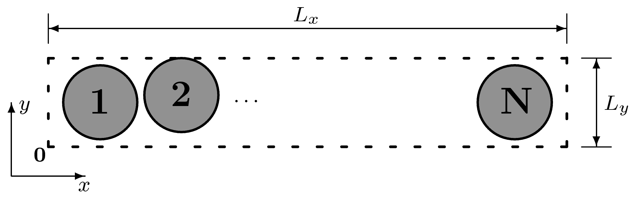
The quasi-one-dimensional (QOD) system introduced recently [16] can be modified to interact with an idealized heat reservoir in a deterministic and reversible way [17], to study heat conduction in low dimensional systems [21] and the Lyapunov mode structure. Similar systems have been used recently to study heat flow [19,20]. This system contains hard disks in a narrow channel that does not allow the disks to change their (left to right) order, see Figure 1.

Figure 1. Schematic of an N hard-disk quasi-one-dimensional (QOD)system. The height $L_y$ is sufficiently small that the disks cannot pass one another. We choose the coordinate origin to be located at the bottom left corner of the system, and system boundaries are denoted by dashed lines. The boundaries at $x=0,L_x$ are hard walls and those at $y=0,L_y$ periodic (that is, a HP quasi-one-dimensional system).

Figure 1. Schematic of an N hard-disk quasi-one-dimensional (QOD)system. The height $L_y$ is sufficiently small that the disks cannot pass one another. We choose the coordinate origin to be located at the bottom left corner of the system, and system boundaries are denoted by dashed lines. The boundaries at $x=0,L_x$ are hard walls and those at $y=0,L_y$ periodic (that is, a HP quasi-one-dimensional system).

The equations of motion connecting the QOD system to the two reservoirs at $x=0,L_x$ define the thermal contact. When a particle collides with a reservoir wall the normal component of the momentum of the particle is changed by

$$p_x^{\prime }=ϵp_I-(1-ϵ)p_x.$$

(9)

$p_I$ is the value of the reservoir momentum for the $I^{th}$ reservoir (either $p_L$ or $-p_R$). If $ϵ=0$ there is no interaction with the reservoir, and if $ϵ=1$ the incoming momentum is completely replaced by the reservoir momentum. Generally we use a value of $ϵ=0.5$ which provides an effective mixing of the incoming momentum with the reservoir momentum, and a density of 0.8. The value of $L_y=1.15\sigma$ and $L_x$ varies with the number of particles N as $N{\sigma }^2/\left(L_x{L}_y\right)=0.8$. For a boundary temperature of $T_I$ the reservoir momentum is given by $p_I=\sqrt{2T_I}$. The temperature profile is determined from the average components of the kinetic temperature of each particle (the average of equation 8 ). As the QOD system is narrow enough to prevent particles interchanging their positions, the order of the particles remains fixed. Therefore, the temperature profiles are shown as functions of the particle number, rather than particle position. Also both x and y components of the temperature are presented together to show the level of local thermal equilibration. 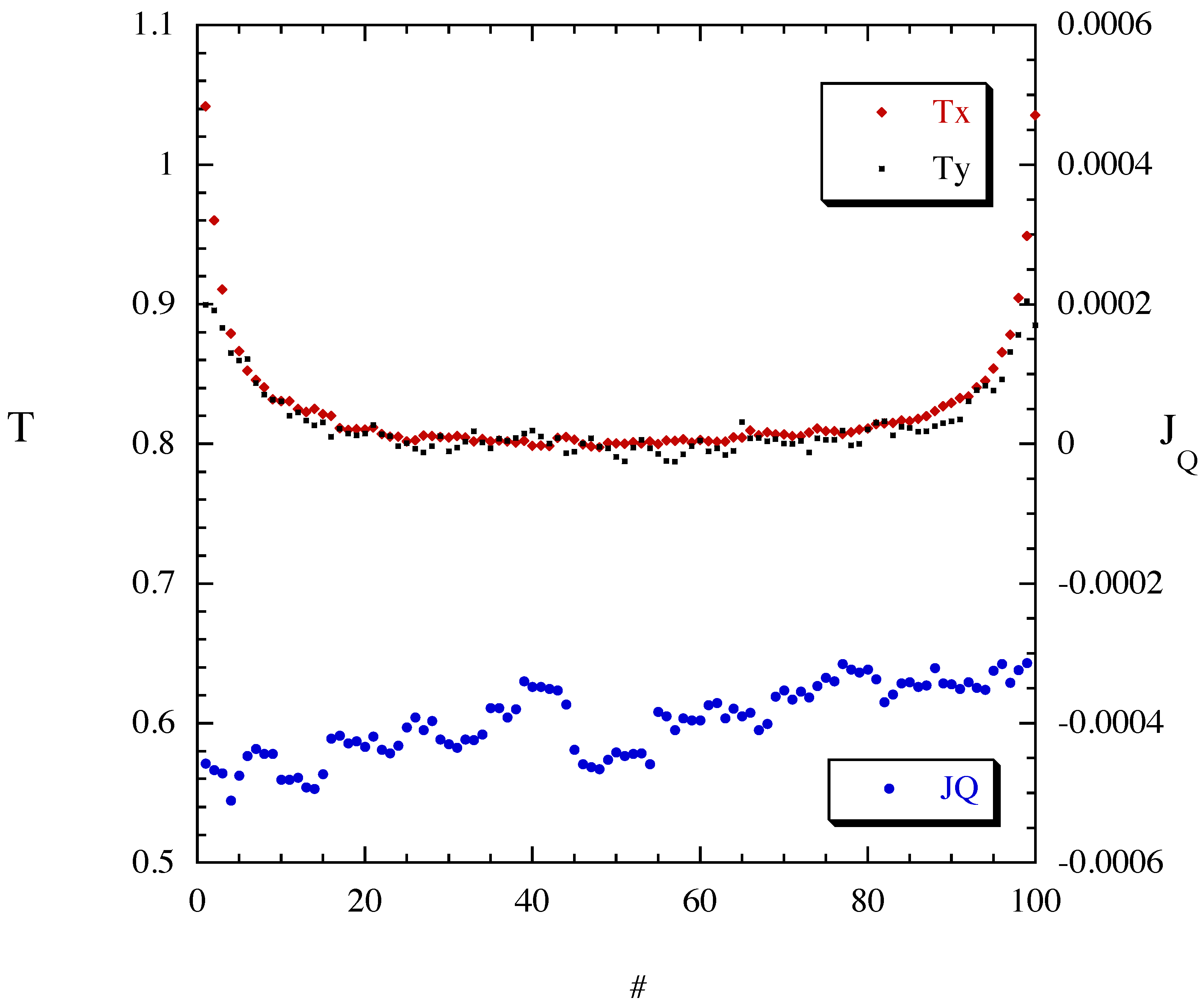Figure 2 shows both components of the temperature profile for a QOD system of 100 disks with reservoirs of temperature $T=1$ on each side.

Figure 2. The temperature profile $T_x$ and $T_y$, and inter-disk heat current $J_Q$ for a QOD system of 100 hard-disks. Notice that the temperature increases near the two reservoirs with the temperature in the centre is about 20% smaller than the nominal reservoir temperature $T=1$. This is termed the contact resistance. There is a very small residual heat current to the left. There is also a noticeable difference between the x and y temperatures of the particles closest to the two boundaries. This arises because the boundary collisions treat x and y components of momentum differently.

Figure 2. The temperature profile $T_x$ and $T_y$, and inter-disk heat current $J_Q$ for a QOD system of 100 hard-disks. Notice that the temperature increases near the two reservoirs with the temperature in the centre is about 20% smaller than the nominal reservoir temperature $T=1$. This is termed the contact resistance. There is a very small residual heat current to the left. There is also a noticeable difference between the x and y temperatures of the particles closest to the two boundaries. This arises because the boundary collisions treat x and y components of momentum differently.

The change in temperature near the contact with the reservoir has been observed before and has been termed the Kapitza resistance [21,22]. Here the centre of this equilibrium system is about 20% colder than the two reservoirs. Numerical calculation of the $p_x$-distribution for the particle in the centre of the system gives a Gaussian distribution with the same temperature as the centre of the profile, as shown in Figure 2. We observe that to a good approximation, the two halves of this Gaussian propagate to the left and the right unchanged. Thus the distribution of incident momentum $p_x$ at each reservoir is Gaussian with the same temperature as the centre of the system. As the system is intended to be at equilibrium with the two reservoirs it is steady when the net energy flow through the boundaries is zero. Thus if p is the momentum before collision with the wall and $p^{\prime }$ is the momentum after collision then $<{p^{\prime }}_x^2-p_x^2>=0$. Using the collision rule in equation (9) and taking the wall momentum as $p_I$, we require

$$ϵ(ϵ-2)<p^2>-2ϵ(1-ϵ)<p>p_I+{ϵ}^2{p}_I^2=0.$$

(10)

The incoming half Gaussian has a mean of $<p>=\sigma \sqrt{\frac{2}{\pi }}$ and a variance of $<p^2>={\sigma }^2$, so inserting these into equation (10), setting $p_I=1$, and solving for the variance of the incoming Gaussian $\sigma \left(ϵ\right)$ gives

$$\sigma \left(ϵ\right)=\frac{1}{2-ϵ}[\sqrt{\frac{2}{\pi }}(1-ϵ)+\sqrt{\frac{2}{\pi }{(1-ϵ)}^2+ϵ(2-ϵ)}].$$

(11)

For $ϵ=\frac{1}{2}$ the temperature is $T={\sigma }^2=0.813$ which is in good agreement with the temperature at the middle of the system.

As the incoming momentum distribution is half Gaussian, using the collision rule in equation (9), we can estimate the outgoing $p_x$ distribution for particle 1 as the weighted convolution of the reflected half Gaussian and the delta function reservoir momentum distribution. Recollisions of particle 1 and 2 will modify this approximate distribution, but for our purposes this will be sufficient. This out-going distribution for particle 1 interacts with the in-coming distribution of particle 2 to generate the out-going distribution for particle 2. We assume that the inputs to this process are two independent random variables so the out-going distribution is the convolution of the two input distributions. Thus for particle 2 the outgoing distribution is the convolution of a half Gaussian and a delta function, with its maximum at $\frac{p_I}{2}$ and half the variance.

To generate approximate distributions for successive particles 3, 4 and 5 etc. we again assume that we can again convolve the out-going distribution of particle i with the incoming distribution of particle $i+1$ to get the out-going distribution of particle $i+1$. With each convolution the maximum of the distribution moves to $\frac{p_I}{2^n}$ and the variance becomes $(1-\frac{1}{2^n}){\sigma }^2$. The contribution to the variance from the outgoing distribution of the $n^{th}$ particle is

$$<p_n^2>=\frac{p_I^2}{2^{2n}}+\sqrt{\frac{2}{\pi }}\frac{p_I}{2^n}\sqrt{1-\frac{1}{2^n}}+{\sigma }^2(1-\frac{1}{2^n}).$$

(12)

Notice that in the limit as $n\to \infty$, $<p_n^2>\to {\sigma }^2$ so the distribution again matches the full Gaussian distribution in the centre of the system. The temperature is then

$$T_n=\frac{{\sigma }^2}{2}+\frac{<p_n^2>}{2}={\sigma }^2$$

(13)

In a numerical calculation the kinetic energy transferred from particle i to particle $i+1$ in each collision can be calculated from

$$\Delta e_{\to }=-\frac{1}{2m}({\mathbf{p}}_{ij}.{\mathbf{r}}_{ij}){\mathbf{r}}_{ij}.({\mathbf{p}}_i+{\mathbf{p}}_j),$$

(14)

where ${\mathbf{r}}_{ij}={\mathbf{r}}_j-{\mathbf{r}}_i$ and ${\mathbf{p}}_{ij}={\mathbf{p}}_j-{\mathbf{p}}_i$. The time average of this quantity gives the average energy current flowing from particle i to $i+1$. Notice that when the total momentum of the two colliding particles is zero, no energy is transferred. The transfer of energy is correlated with fluctuations of the pair momentum away from zero.

3.2. Nonequilibrium

Figure 3 shows the temperature profile for a nonequilibrium QOD system in an external temperature gradient $T_L=3$ and $T_R=2$. The contact resistance is again evident at both boundaries, both the hot boundary and the cold boundary. The mechanism that produced this effect in the equilibrium case occurs again, but now modified by the temperature gradient. The incoming distributions will be Gaussian but with a variance that changes slowly with position. This is due to the local equilibration of the energy between x and y coordinates of the same particle as evident in Figure 3, leading to the x and y components of the temperature of each particle being approximately equal.

Figure 3. The temperature profile and inter-disk heat current $J_Q$ for a nonequilibrium QOD system of 100 hard-disks with $T_L=3$ and $T_R=2$. Notice that the contact resistance is evident at both reservoirs. Due to the temperature difference there is a heat current of $J_{Qx}=0.245$ to the right.

Figure 3. The temperature profile and inter-disk heat current $J_Q$ for a nonequilibrium QOD system of 100 hard-disks with $T_L=3$ and $T_R=2$. Notice that the contact resistance is evident at both reservoirs. Due to the temperature difference there is a heat current of $J_{Qx}=0.245$ to the right.

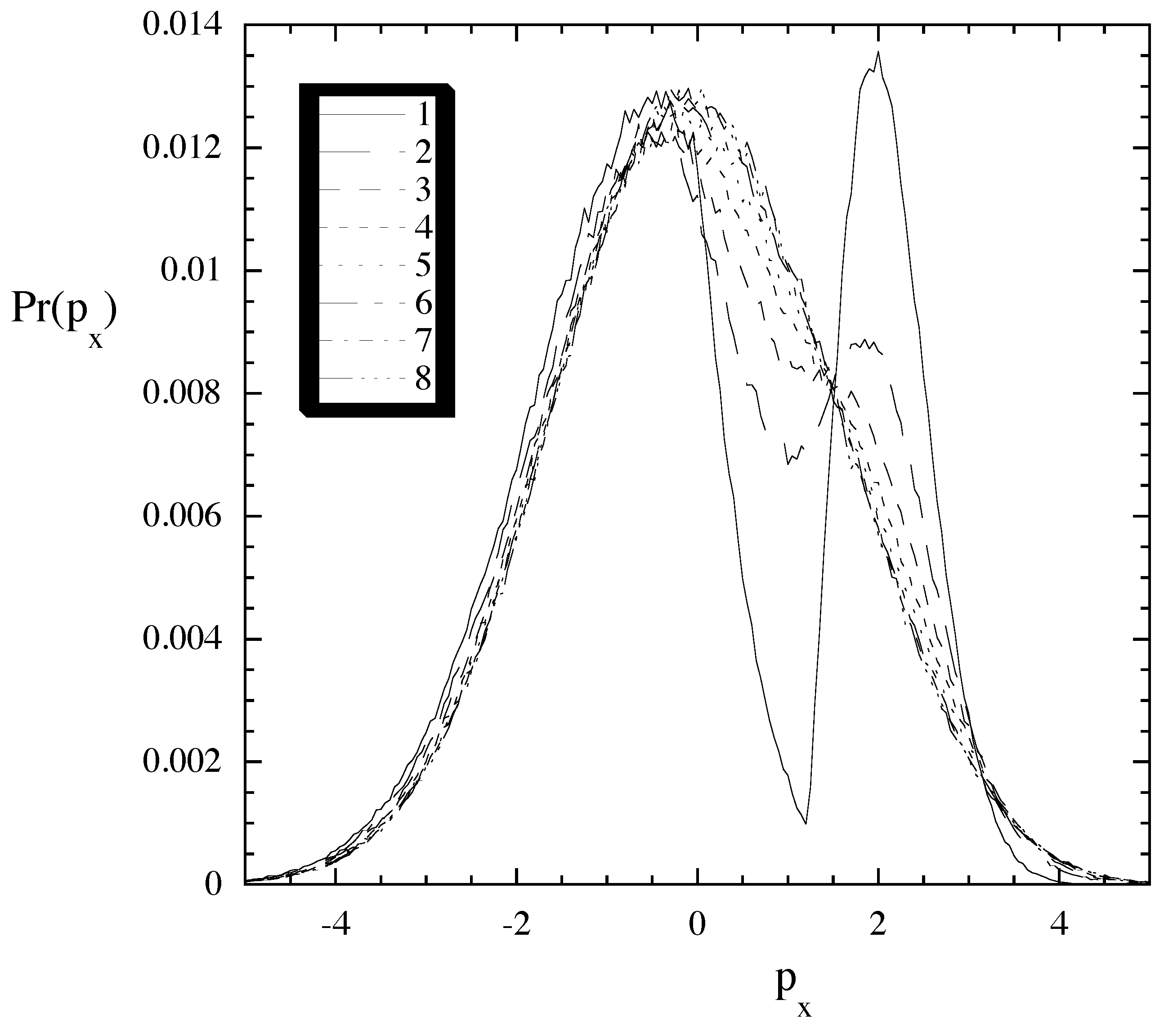
The process is clear when we look at the distributions of $p_x$ for the first eight particles on the left-hand side of the system in Figure 4. These are the particles closest to the hot reservoir. The incoming distributions are again approximately Gaussian, and the out-going distributions show the same behaviour as the equilibrium system. For particle 1, the distribution is changed by the collision process at the boundary, but for particle 2 this diminishes and each successive particle distribution diminishes the effect of the wall even more, until at particle 8 the whole distribution looks almost completely Gaussian again. While the momentum distributions cannot be exactly Gaussian because this nonequilibrium system supports an energy current, the deviations from Gaussian are at best only subtle.

Figure 4. The probability distribution for the x component of the momentum for particles 1 to 8 in the nonequilibrium QOD system shown in figure (3). These are the particles nearest the hot reservoir. The incoming distributions (the negative part of the $p_x$ distribution) are very close to Gaussian for each particle, while the outgoing distributions show the same qualitative behaviour as the outgoing distributions in the equilibrium case. There is a strong effect in the outgoing distribution of particle 1, and that effect successively diminishes in particles 2, 3, etc. as the distribution slowly returns to its approximately Gaussian shape.

Figure 4. The probability distribution for the x component of the momentum for particles 1 to 8 in the nonequilibrium QOD system shown in figure (3). These are the particles nearest the hot reservoir. The incoming distributions (the negative part of the $p_x$ distribution) are very close to Gaussian for each particle, while the outgoing distributions show the same qualitative behaviour as the outgoing distributions in the equilibrium case. There is a strong effect in the outgoing distribution of particle 1, and that effect successively diminishes in particles 2, 3, etc. as the distribution slowly returns to its approximately Gaussian shape.

3.3. Stochastic Models

Eckmann and Young [18] have developed Hamiltonian and stochastic models for heat transport in low dimensional systems. The Hamiltonian models consist of energy storage devices which couple to each other through the motion of tracer particles that carry the energy. Although these models principally store energy as rotational kinetic energy, they are similar in many ways to the QOD system that we consider. The Lorentz gas can be considered to be the model obtained by taking two disks on a torus and expanding one disk to twice its diameter and shrinking the other to a point. In this way the interaction between the scatterer and point is the same as the interaction between the two disks. In a similar way, expanding all the even numbered disks and contracting all the old numbered disks in the QOD system, leaves the interaction between neighbouring disks the same. The transformed QOD system then resembles an array of scatterers (the even numbered disks) with a tracer particle between each pair (the odd number disks), except that the QOD system does not lead to equally spaced scatterers. Therefore it is reasonable to suppose that the QOD system may be in the same universality class as those considered by Eckmann and Young and their result for the temperature profile of the system may be valid. That is

$$T\left(x\right)={(T_L^{\alpha }+(T_R^{\alpha }-T_L^{\alpha })x)}^{\frac{1}{\alpha }},$$

(15)

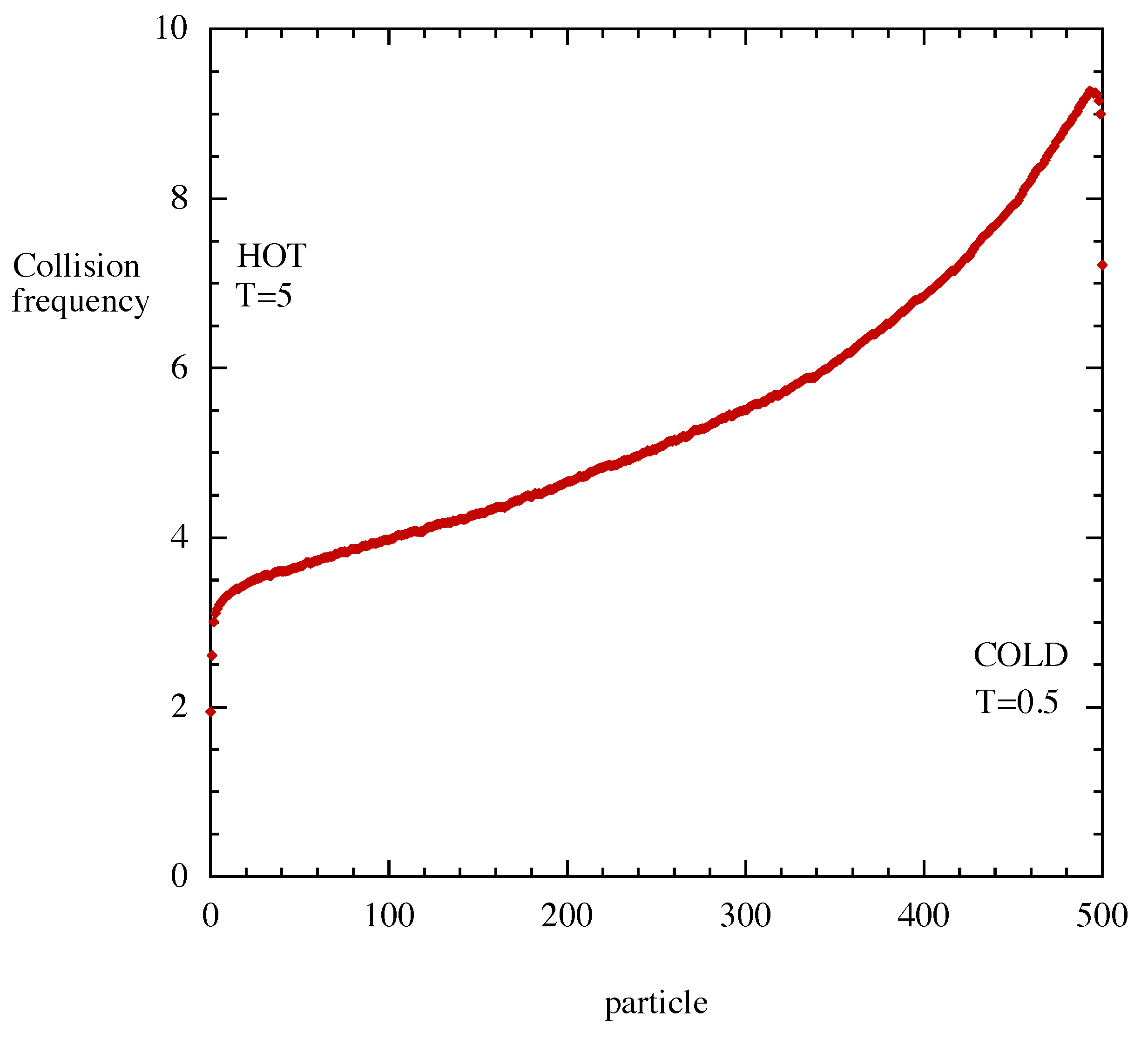
where $T_L$ and $T_R$ are fixed the temperatures at the left and right ends, and x goes from 0 to 1 as we move from the left end to the right end. The constant α depends on the nature of the coupling, and if the energy is purely kinetic a value of $\alpha =\frac{3}{2}$ is expected. The model is based on two very reasonable assumptions: that energy is shared in tracer-scatterer collisions, and that the speed of the tracer particles is proportional to some power of their kinetic energy. Therefore we would expect the speed and collision frequency to be highest near the hot reservoir and lowest near the cold reservoir. The rate at which a tracer does a cycle of interaction (interacting with both its neighbours) is the inverse of the time it takes to do two collisions. In a molecular dynamics simulation of the QOD system in Figure 5 we observe exactly the opposite effect. The collision frequency is greatest near the cold reservoir and smallest near the hot reservoir.

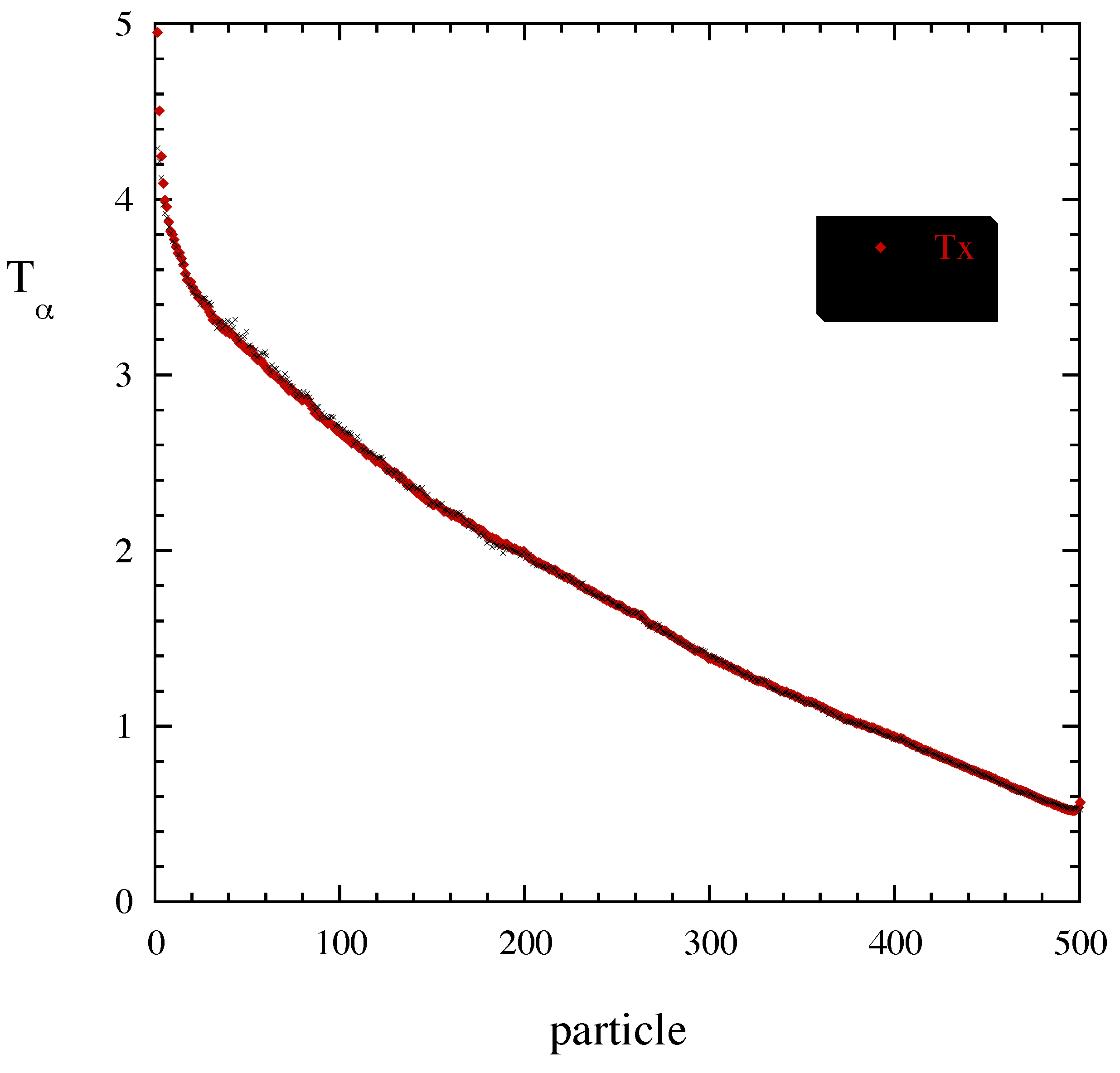
In Figure 6 we present the temperature profile calculated in the simulation. Clearly the temperature profile must decay from a value of $T=5$ at the left-hand boundary to a value of $T=0.5$ at the right-hand boundary. From the results of Eckmann and Young we expect a value of $\alpha =\frac{3}{2}$, whereas the observed temperature profile in Figure 6 implies a value of $\alpha <1$. Further, even fitting the observed temperature profile to the function given in equation (15) with α unconstrained gives a very poor fit. The assumption that is made about the collision rate in the stochastic model, although reasonable, is not correct for this system. One possible reason for this discrepancy may be the fact that the temperature gradient in the QOD system produces a density gradient where the hot region is less dense than the cold region. This would lead the QOD system to give tracer-scatterer system non-equally spaced scatterers.

4. Conclusion

We have investigated the consequences of a particular model microscopic coupling of a system to a reservoir. The advantages of the model include its relative simplicity and the fact that it is deterministic. The model coupling mechanism produces a contact resistance in the kinetic temperature at the boundaries between the system and the reservoirs in both equilibrium and nonequilibrium situations. This contact resistance in the kinetic temperature is commonly observed in the computer simulations of low-dimensional heat conduction [21].

The expected equilibrium configuration of a system between two reservoirs of the same temperature leads to a system that has a steady kinetic temperature which is lower than the temperatures of the reservoirs. By considering the probability distributions of the momentum of particles near the boundary, and the details of the reservoir dynamics, we provide a microscopic explanation of this effect. The appearance of a kinetic temperature gradient near the boundary of an equilibrium system with no associated heat current implies that the kinetic and thermodynamics temperatures are different in this region. We take as our definition of the thermodynamic temperature, that property whose gradient produces a heat current, so the observation of no heat current in the system implies that the thermodynamic temperature is constant everywhere in the system. The thermodynamic temperature is thus defined indirectly and we are unable to write it in terms of microscopic variables. The kinetic temperature difference across the boundary of an equilibrium system, makes the idea of stablising systems to some target temperature, by placing it in thermal contact with a reservoir, more difficult than expected. To achieve a certain target system kinetic temperature the temperature of the reservoir has to be higher. The Kapitza effect observed in nonequilibrium systems with a heat flow, may also be an artifact of the difference between kinetic and thermodynamic temperatures.

Figure 5. The collision frequency for each disk in a nonequilibrium QOD system of 500 hard-disks. The left reservoir has $T_L=5$ and the right reservoir has $T_R=0.5$. Notice that the collision frequency is largest near the cold reservoir and smallest near the hot reservoir. There is a heat current from left to right.

Figure 5. The collision frequency for each disk in a nonequilibrium QOD system of 500 hard-disks. The left reservoir has $T_L=5$ and the right reservoir has $T_R=0.5$. Notice that the collision frequency is largest near the cold reservoir and smallest near the hot reservoir. There is a heat current from left to right.

Stochastic modeling of the heat conduction process for related Hamiltonian systems does not agree with molecular dynamics computer experiments presented here for the QOD system. We have identified the assumptions made in the stochastic treatment of a seemingly similar system that do not apply for the QOD system. We conclude that applying a temperature gradient to the QOD system induces a density profile, so that the QOD system can no long be approximated by a periodic scatterer-tracer system. We believe that this may be the reason that the stochastic assumptions applied to scatterer-tracer system do not hold for the QOD system.

Figure 6. The temperature profile in a nonequilibrium QOD system of 500 hard-disks with $T_L=5$ and $T_R=0.5$. The x component of the temperature has red symbols and the y component of the temperature has black symbols. The x and y temperatures are approximately equal for each particle even though there is a strong temperature gradient in the system.

Figure 6. The temperature profile in a nonequilibrium QOD system of 500 hard-disks with $T_L=5$ and $T_R=0.5$. The x component of the temperature has red symbols and the y component of the temperature has black symbols. The x and y temperatures are approximately equal for each particle even though there is a strong temperature gradient in the system.

References and Notes

1. Hatano, T.; Sasa, S. Steady-State Thermodynamics of Langevin Systems. Phys. Rev. Lett. 2001, 86, 3463. [Google Scholar]
2. Morriss, G.P.; Rondoni, L. On a Definition of Temperature in Equilibrium and Nonequilibrium Systems. Phys. Rev. E 1999, 59, 5. [Google Scholar] [CrossRef]
3. Baranyai, A. Numerical temperature measurement in far from equilibrium model systems. Phys. Rev. E 2000, 61, 3306. [Google Scholar] [CrossRef]
4. Baranyai, A. Temperature of nonequilibrium steady-state systems. Phys. Rev. E 2000, 62, 5989. [Google Scholar] [CrossRef]
5. Jou, D.; Casas-Vazquez, J.; Lebon, G. Extended Irreversible Thermodynamics; Springer: Berlin, 2001. [Google Scholar]
6. Ottinger, H.C. Beyond Equilibrium Thermodynamics; Wiley: New York, 2005. [Google Scholar]
7. Ritort, F. Resonant Nonequilibrium Temperatures. J. Phys. Chem. B 2005, 109, 6787. [Google Scholar] [CrossRef] [PubMed]
8. Garriga, A.; Ritort, F. Mode-dependent nonequilibrium temperature in aging systems. Phys. Rev. E 2005, 72, 031505. [Google Scholar] [CrossRef]
9. Shokef, Y.; Shulkind, G.; Levine, D. Isolated nonequilibrium systems in contact. Phys. Rev. E 2007, 76, 030101. [Google Scholar] [CrossRef]
10. Gruber, Ch.; Frachebourg, L. On the adiabatic properties of a stochastic adiabatic wall: Evolution, stationary non-equilibrium, and equilibrium states. Physica A 1999, 272, 392. [Google Scholar] [CrossRef]
11. Callen, H.B. Thermodynamics; Wiley: New York, 1960. [Google Scholar]
12. Thompson, C.J. Mathematical Statistical Mechanics; Macmillian: New York, 1972. [Google Scholar]
13. Morriss, G.P.; Daivis, P.J.; Evans, D.J. The Rheology of n-alkanes: Decane and Eicosane. J. Chem. Phys. 1991, 94, 7420. [Google Scholar] [CrossRef]
14. Evans, D.J.; Morriss, G.P. Statistical Mechanics of Nonequilibrium Liquids, 2nd Edition ed; Cambridge University Press: Cambridge, 2008. [Google Scholar]
15. Evans, D.J. On the Entropy of Nonequilibrium States. J. Stat. Phys. 1989, 57, 745. [Google Scholar] [CrossRef]
16. Taniguchi, T.; Morriss, G.P. Boundary effects in the stepwise structure of the Lyapunov spectra for quasi-one-dimensional systems. Phys. Rev. E 2003, 68, 026218. [Google Scholar] [CrossRef]
17. Taniguchi, T.; Morriss, G.P. Lyapunov Modes for a Nonequilibrium System with a Heat Flux. Comptes Rendus Physique 2007, 8, 625. [Google Scholar] [CrossRef]
18. Eckmann, J.P.; Young, L.S. Temperature profiles in Hamiltonian heat conduction. Europhysics Lett. 2004, 68, 790. [Google Scholar] [CrossRef]
19. Deutsch, J.M.; Narayan, O. One-dimensional heat conductivity exponent from a random collision model. Phys. Rev. E 2003, 68, 010201. [Google Scholar] [CrossRef]
20. Deutsch, J.M.; Narayan, O. Correlations and scaling in one-dimensional heat conduction. Phys. Rev. E 2003, 68, 041203. [Google Scholar] [CrossRef]
21. Lepri, S.; Livi, R.; Politi, A. Thermal conduction in classical low-dimensional lattices. Phys. Rep. 2003, 377, 1. [Google Scholar] [CrossRef]
22. Lumpkin, M.E.; Saslow, W.M.; Visscher, W.M. One-dimensional Kapitza conductance: Comparison of the phonon mismatch theory with computer experiments. Phys. Rev. B 1978, 17, 4295. [Google Scholar] [CrossRef]