1. Introduction
Given a sample of statistical data, the maximum entropy method (MEM) is commonly employed to construct an analytical form for the probability density function (pdf) in myriad applications across a diverse array of disciplines [
1,
2,
3]. The classic problem has been posed as: Given a finite set of power moments over the random variable,
x, defined as
,
; find a pdf that reproduces these power moments. Unfortunately, this problem is ill-posed because it is clear that a finite number of moments cannot lead to a unique pdf. Moreover, if a sequence of such moments is arbitrarily specified, it is possible that no pdf can be constructed because there exists well-known inequality relations that must be satisfied among the moments when they are derived from any true pdf. For example, if the assumed pdf is bounded on a finite interval, the construction of the pdf is referred to as the Hausdorff moment problem, which remains a highly active research area in statistics and probability theory [
4,
5,
6,
7] in regards to finding the most faithful pdf when only limited information about the moments is known.
The problem of interest in this paper is much simpler than the Hausdorff moment problem because the collected statistical data ensures that a pdf exists. For example, the pdf can be directly estimated by making a histogram of the statistical data. Although the histogram method may provide a sufficient estimate for the pdf, its analytical form will be unknown. To determine an analytical form, a common approach is to calculate the set of power moments
from the sampled statistical data, and apply the postulate that the true pdf will maximize entropy while satisfying the set of constraints that all known moments will be reproduced. As such, the MEM is useful because it recasts an ill-posed inverse problem into a well-defined calculus of variation problem. Although other methods are available that do not invoke the maximum entropy assumption [
8], it has been shown that the MEM generally is able to obtain a pdf with the same degree of accuracy using less number of moments [
9].
Due to the appeal of the MEM, and its connection and origins with statistical physics concepts [
10], many inverse problems encountered in physics have been successfully solved [
11] using a markedly small number of moments. As powerful as the MEM has proven to be, it has been notoriously difficult to find stable algorithms to reconstruct the pdf when the number of known empirical moments become more than four [
12,
13,
14]. This problem is unfortunate, because in principle a more accurate pdf can be determined the greater number of moments that are known. The common attribute of numerical methods that have problems with convergence and stability require employing a Hessian matrix to find a minimum of a function of many variables (being the set of Lagrange multipliers that appear from the calculus of variation problem). Interestingly, much greater numerical stability has been achieved by considering moments of certain types of orthogonal polynomials where the zeros of all the polynomials are within the domain range of the random variable,
x, such as the Chebyshev polynomials [
15] appropriately scaled on a bound interval. Recently, a robust method has been developed that has been demonstrated to be stable using hundreds of moments [
16]. Although using moments of orthogonal functions achieve greater numerical stability compared to power moments, convergence problems remain, and this approach is not completely robust. Rather than viewing a set of moments as characterizing a pdf, the histogram of the sampled data has been directly used as constraints within the framework of the MEM [
17]. The maximum entropy histogram approach appears to be robust.
In this paper, a combination of the orthogonal function moments and the maximum entropy histogram approach are combined to yield a novel MEM variant that is robust. The motivation for developing a new MEM was to determine a pdf with high accuracy that extends deep into the tails of the distribution function, where the sampling is very sparse. The specific application of interest is related to the calculation of a partition function at temperature,
T, given that the probability density of finding a system in a state of energy,
E, while subject to a thermal bath at temperature,
, is given by
. It is straightforward to derive the partition function is given as
where
is the lowest possible energy of the system,
, and
k is the Boltzmann constant. In this application of interest, the sampling of
E was obtained using Monte Carlo (MC) simulation at
, and from this data, an accurate pdf was sought. Thermodynamic functions, such as free energy, mean energy, entropy and heat capacity are then calculated from
. For these quantities to be accurate at temperatures,
T, far away from
, the pdf must be accurate in the tails at both low and high energy,
E. The new MEM that was developed to solve this problem was verified to work well, because the MC simulations were performed at other temperatures as a direct check. Although it is possible to simply run MC simulation for all temperatures of interest, the approach defined in Equation 1 provides analytical expressions, which were desired.
The focus of this paper is to describe the novel MEM in a general context because determining an accurate pdf from sampled data is ubiquitous. In particular, in many applications the true answer is not known, and it is impractical to simply sample more to obtain better accuracy within the tails. Therefore, consider the generic problem that requires re-weighting the pdf with exponential factors, such that
where
is an arbitrary function,
is the unknown pdf that is to be determined, and
μ is essentially a conjugate Laplace transform variable. One problem with Equation 2 is that
could have high powers of
x, or
, making the average
very sensitive to noise in the sampling data. More difficult is the exponential re-weighting factor that increases the significance in the tails of the original pdf that were low probability regions. This sort of problem had to be solved in some practical way. Obviously, any method will break down at some point for
too large, or for some misbehaved function. Therefore, the first approach was to simply smooth the original sampled data using a sliding histogram smoothing technique. However, when attempting to re-weight the pdf while working with moments dealing with powers of
, the smoothing/histogram method failed to yield satisfactory results. Failure in using a smoothed distribution function was confirmed by performing numerical experiments where the exact
function is known. This null result suggested to apply some standard MEM that was already available. Unfortunately, the method that promised to be very robust [
16] failed to work. It was this discouraging result that required reformulating the problem so that a solution for the pdf, given the existence of the histogram, would always be possible.
In this paper, I present a solution to the problem of constructing the pdf from statistical data that works remarkably well for applications described by Equation 2. The MEM presented is pragmatic in nature, using a combination of computational and optimization methods. I provide no proofs that the method presented is optimal, as it appears one could create many variants to work just as good. In my original application of interest, no a priori information about the true pdf is known, except that the pdf exists in the form of a histogram, and the lower limit in x is bounded, but this value is unknown. In this paper, the method is developed to allow for either the lower and upper limits in Equation 2 to be finite or not. The conclusion is what one should expect. First, the method will always return a result. The final pdf that is returned can reproduce the original statistics observed from the sampled data. Extrapolating the moments using Equation 2 will almost surely be in error for most problems if one exceeds reasonable limits on . However, for reasonable extrapolations, the method is probably the best one can hope for. That is, an analytical form for the pdf is always constructed that allows for accurate integration of -moments, and the sensitivity of the re-weighted moments can be controlled to a point, which provides a means to estimate uncertainties in the predictions. Thus, the method presented is a robust way to solve a common problem regarding constructing probability density functions, and calculating averages of functions.
A key feature of the new method described here is that the constraints are not considered to be exact. This is because one must realize that the power moments or moments of orthogonal functions carry with them error bars that reflect the number of independent samples taken. This error due to limited sampling is also present in the histogram. In particular, when the sampling is very limited, there is large intrinsic noise due to unavoidable fluctuations. Methods that rely on exact known values of certain moments can be expected to have problems because of the uncertainties within the constraints. Recent work has been done in trying to correct for intrinsic noise that appears due to limiting sampling [
18,
19,
20]. The approach taken here is to spread errors due to inconsistencies that originate from fluctuations in sampling over all the constraints being imposed. In other words, all the constraints are softened by minimizing the least squares error between the final predicted moments with the empirically derived moments that are operationally calculated from the statistical data. The advantages of the least squares approach in the context of determining a pdf has also been considered before [
21].
The new MEM described here yields the “best” pdf for quantitatively representing statistical data. This claim is made because many constraints are considered simultaneously, which includes a large number of moments, as well as requiring the pdf to reproduce the histogram. The method is set up in a generic fashion, meaning nothing special needs to be known about the nature of the pdf. However, when the sample dataset is small, the predicted pdf can substantially deviate from the true pdf. Nevertheless, the method is robust in the sense that it always returns a pdf that reproduces the statistics while gracefully distributing statistical uncertainties. It is demonstrated that as the number of samples increases, the predicted pdf converges to the true pdf markedly well, even for difficult cases.
2. Method
This section is broken down into a step-by-step prescription for a novel MEM, where each step is a straightforward exercise. First, the sampled data is transformed to reside on a finite interval, which makes the subsequent analysis much easier. Consequently, the pdf of the transformed data is subject to the Hausdorff moment problem. Second, rather than using power moments which tend to loose useful information across the entire domain range as the power increases, the moments for a set of orthogonal level-functions is much more appropriate because all regions within the domain range of the random variable are covered more uniformly. Third, the least squares error method is formulated such that the constraints need not be perfectly satisfied, but rather all constraints should be satisfied as best as possible by distributing the residual errors over all the imposed constraints. These constraints include matching to the histogram, where the binning size is properly taken into account. Fourth, a discussion of how to handle boundary conditions is given. Fifth, a method for smoothing the pdf is described that adds additional constraints to the least squares method. In this way, smoothing is handled with ease, and the degree of smoothing can be controlled by the user at the expense of increasing errors between empirical based moments and the calculated moments from the predicted pdf. Sixth, a simulated annealing technique is proposed to avoid dealing with ill-behaved Hessian matrices that cause numerical instability. The method implemented prevents over specifying Lagrange multipliers, which is determined by monitoring how the least squares error decreases as more Lagrange multipliers are included. In the seventh step, a novel type of adaptive simulated annealing technique, called funnel diffusion is described, which was implemented in this work. The description of these seven prudent steps will hopefully become a valuable resource for those who would like to either use the method presented as is, or further explore variations.
2.1. Transforming the sampled data
The situation envisioned deals with statistical data,
, consisting of
N unbiased observed random events. Whether true or not, initially it is assumed that the range of accessible values of
x is over all reals
. However, the probability of observing an
that is an extreme outlier approaches zero rapidly, and thus the tails of the pdf are not sampled well. The lowest and greatest observed values define
and
respectively. All random data is mapped onto an interval that has a range
through the transformation
By setting
for
on the interval
; Equation 3 maps all
N observed data points onto the
smaller interval between
, where
is free to be set to a desirable value. Since
for
, selecting a small value for
will keep the transformation essentially linear. However, small
will compress all the data into a local region near the origin, and resolution is lost. Resolution means that if a curve having minimums and maximums is squeezed down into a very small region,
, a set of orthogonal functions that span the range
will accurately represent the curve only if they vary rapidly over short scales. Thus, to keep the need to resolve small scales to a minimum, it is best to spread the data over the entire range available. On the other hand, although large
yields greater resolution for most of the data, resolution in how the curve varies will be lost in the tails of the distribution where the transformation is non-linear in the regime where
. Keeping the resolution problem in mind on both sides, a value near
for
works well. However, when the data is binned, it is best to not have any possibility that the data falls exactly on the boundary. To prevent data to lie on the boundary during the binning process, it is numerically convenient to shift the limiting
value to be infinitesimally smaller than the nominal value would otherwise indicate. A slight shift guarantees that the binning scheme that is to be employed below will maximally cover the domain range of
y, but if the shift is large, then it is possible that the bins defining the boundary will be unfilled with data. Although normally these details are not a concern, it was found that careful attention to the boundaries of bins is necessary in order to maintain high accuracy when singularities are present at a boundary. To provide a robust generic method, a slight numerical shift proved sufficient to accurately describe singularities that occur at these boundaries. Denoting
ϵ as a very small number, such as
, a value of
is found to work well in transforming the data while avoiding problematic concerns. Then,
with this choice of
, and the sampled data lies on the range (
). Alternatively, another logical choice is to set
where
is the mean value of the sampled data, and
where
is the standard deviation. In most cases good results occur using either prescription of change of variable. However, the transformation presented in Equation 3 is much better when the distribution is highly skewed to the far left or right.
The transformation of Equation 3 is applied to all input data to produce a new set of random variables given by
. Note that the new variables are dimensionless. Let
define the pdf for the
transformed random variables,
. The objective now becomes determining
using the MEM. The advantage of using the variable
y is that it is known to be bound on the interval
. After
is found, the inverse transformation is applied to arrive at
The form of Equation 4 makes the tails of
fall off extremely fast for large values of
x due to the
function in the denominator. This functional behavior at the boundaries is fully welcomed and desirable to guarantee that the predicted
is normalizable.
2.2. Maximum entropy method applied to level-functions
Consider a set of functions that are labeled as
. Based on the dataset
the empirical and theoretical moments of these functions are given as
Although we do not know what the pdf is, a reasonable constraint to place on the function
is for the theoretical and empirical averages of a large set of functions to be equal. Other than satisfying all these moment conditions and the normalization condition, it is convenient to assume the functional form of
will maximize information entropy. There is of course no justification for this assumption, except what it does pragmatically. By maximizing the Shannon entropy, given by
, the distribution function will be as broad as it possibly can be to maximize this entropy term, while maintaining the other equalities. As such, the function
can be determined using the calculus of variation by finding the maximum of the functional given by:
where
and the set,
, are Lagrange multipliers. Once the Lagrange multipliers are determined, the general form of
is simply given by:
The MEM shows the generic form of the pdf is an exponential of a linear combination of the moment-functions used in observations. It is common to consider a set of functions that are elementary powers of y, such as y, , , . Alternatively, the moment-functions could also be polynomials, such as . Each of these polynomial functions (of all different sorts) are associated with its own Lagrange multiplier as shown in Equation 6. In either case, the solution using the MEM for is the exponential of a polynomial function. Based on the generic form given in Equation 7, the Lagrange multipliers can be grouped together in algebraic combinations to form a single coefficient per power of y to yield a power series, which in practice is truncated to some highest order term deemed important.
The choice of using polynomials for the moment-functions is not necessary, but the best reason for this choice is because working with a power series is convenient for a generic solution to a general problem. Without knowing specific details to motivate using exotic non-analytic functions, they are best avoided. Having said this, even after the Lagrange multipliers are grouped together to form a generic power series, the choice of moment-functions is important. In general, selecting elementary powers of y is not good, since higher powers probe less of the function for . It is better to probe regions of as uniformly as possible. To this end, it is prudent to use multiple level-functions that more uniformly span different regions in the interval . Note that a level-function means that its absolute value is bound, usually expressed as . Example level-functions are the Chebyshev polynomials, , Legendre polynomials, and sine, and cosine functions, , among many other possible choices. In this work, these four types of level-functions are employed, for integer n from 0 to 20. Notice that in the four examples, the level functions define an orthogonal set of functions. Orthogonality is a desirable property, since each additional condition (enforced through the Lagrange multiplier) is distinct from all previous conditions. Consequently, orthogonality provides the desired feature of uniformity, which is not the case when using the power basis, .
A polynomial will be obtained regardless of whether a few or multiple sets of orthogonal level-functions are used to determine the form of
. Moreover, this polynomial is expected to be truncated to a maximum power, up to
. In this case, the polynomial is expressed exactly in terms of the Chebyshev polynomials. Note that there is nothing fundamentally special about using the Chebyshev polynomials compared to the sine and cosine functions, or the Legendre polynomials over the interval
. However, sine and cosine functions have powers to infinite order, so they were not selected. It is also generally true that Chebyshev polynomials have the best convergence properties among similar finite power series polynomials. Nevertheless, any choice of orthogonal polynomials is expected to work, but determining what the optimal choice is, has not been attempted. With the selection of the Chebyshev polynomials, the general solution for
that maximizes the Shannon entropy while all theoretical moments are constrained to the empirically observed moments is given by
The coefficients
reflect the series expansion for the optimal polynomial function needed to match the empirical moments. Note that if it happens that
is a Gaussian distribution, then it follows that
where
An important point is that higher power moments of a pdf may be fully described by Equation 8 with
found to have
m small. In other words, it is not a priori required to have more non-zero
just because higher moments are calculated and enforced by Lagrange multipliers. If more expansion coefficients are necessary, then surely the higher order level-function moments are critical to determine these coefficients accurately. On the other hand, it can happen that new information about the form of the pdf may appear when higher moments are considered, not because of principle, but because of unwanted sampling noise.
Nominally, the best solution for is expressed by Equation 8, but the values of the expansion coefficients still need to be determined. Unfortunately, the solution will be sensitive to noise in the random sampling. For example, for sampled data points, a certain set of m expansion coefficients, will fit the specific set of observed points. However, for another completely independent set of sampled data points, a different optimal set of expansion coefficients, will in all likelihood be obtained. Thus, sampling noise renders finding an exact solution impossible. Even within a single dataset sampled, the ability for Equation 8 to satisfy an arbitrarily large number of moment-functions may become impossible because m is truncated too soon. Therefore, the criteria of a good representative pdf must be changed from solving the functional given in Equation 6 with an exact set of Lagrange multipliers, to finding an optimal approximate set of expansion coefficients , and optimal number of coefficients from Equation 8. This is conveniently implemented by minimizing the least squares error between all corresponding empirical and theoretical moments simultaneously, where the majority of moment-functions considered are not explicitly represented within the function .
2.3. Least squares error method and integral evaluation
The algorithm that is to be applied to determine the expansion coefficients, , is based on an iterative approach of random guessing. Actually, m is guessed, is guessed for all j such that , and is determined by the normalization condition. For a given set of expansion coefficients, a weighted least squares error, E, for a collection of target conditions is calculated, and used as an objective function. The goal is to guess the set such that . The details of the employed iterative guessing procedure (funnel diffusion) will be described below. Here, consider as given. The dependence on the expansion coefficients is explicitly expressed by writing the function as, .
The generic form of the objective function is given by
where
is a separate objective function for smoothing. Take
when no smoothing is desired. The scale factor
is used to weight the overall importance of the
j-th type of level-function. The selected level-functions,
, include the four types of orthogonal functions described above (
i.e.,
). For these four orthogonal functions, the
n-index specifies the mode for which the greater value of
n implies a greater degree of oscillation and greater number of zero crossings on the interval (-1,1). At some point, appreciable oscillations occur on a scale,
, while
will be approximately constant for the same
. This means that
for large
n. The weight factor,
, can formally represent a cutoff, such that
, and
. However, better results were obtained when moments with (lower, higher)
n are assigned a (greater, lesser) weight. In particular, for
the scale factors were set as
, and
were set with an identical exponential decay of
. With the mode index range of
, this exponential decay sets moments with
a weight of 1, and for
the weight factor is
.
Two more level-functions related to the frequency counts of sampled data (for
) are also included in Equation 10. Perhaps the most common way to estimate a pdf from unbiased sampled data is to construct a histogram using a fixed binning scheme. For the
n-th bin, there will be a count of observations,
. The total number of observations,
N, is given by the sum rule,
. The frequency for finding a random event within bin,
n, is given by
. With respect to the transformed
y-variable, the binning function
is defined as
when
y falls within bin
n, and
when
y is not within bin
n. The empirical estimate is matched with the theoreticalprediction (for
) as
where
is the counts with respect to the
y-variable. A similar pair of equations (for
) is given as
where
in Equation 12 is understood to represent counts with respect to the
x-variable. The relative weighting to match the empirical frequency based on the normalized histogram method to the integrated pdf within corresponding bins has in this work been set to
for
j either 5 or 6.
The number of bins to construct the histogram in the
y-variable was selected to be 40, and 50 bins were used for the
x-variable. In the former case, the bin width is always 0.05 and the 40 bins cover the range (-1,1). The transformation given in Equation 11 for the
y-variable should be commensurate with the bin boundaries. For example, the bin that spans the
y-values between
and
is fully sampled because care was given to make sure
does not fall anywhere other than at the very end of this bin. There is no similar concern for the
x-variable because no artifact from a transformation equation is present to cause a problem. Therefore, the number of bins span the range between
and
, so that
is the bin width. On the theoretical side, integrals given in Equations 5, 11, 12 are discretized. For the problems considered here, it was found that using the Riemann sum of calculus with
points is sufficient, where
Note that because the reference points used in the Riemann sums are centered, the above choice of bin number and
give five Riemann terms for every bin estimating
where
and four Riemann terms for every bin estimating
, where
. Note that it is necessary to make sure the bin resolution for doing this numerical integration is commensurate with the bin resolution for histograms in the
y- and
x-variables. It was found that this resolution is good enough to make sums and integrals virtually indistinguishable. However, more sophisticated numerical methods for estimating integrals should be incorporated if the integrand varies wildly.
2.4. Boundary conditions
There are two possible boundary conditions for at negative y-values (i.e., left, L) and at positive y-values (i.e., right, R). These are either that , or to a limiting value corresponding to a minimum or maximum value in x for the L- or R-sides respectively. If a limiting value is known, it can be specified and used directly to scale the sampled data in Equation 3. In absence of knowing what the limiting value is, other than it exists, the lowest observed value from sampling is used. In either case, all the sampled data representing always falls between . The consequence of enforcing a finite boundary is that when calculating the least squares error given in Equation 10—the range is restricted to be within the physically realizable domain, and outside this domain.
When the boundary condition corresponds to an unlimited range in x-values: Say for the R-side where implying , the function is truly unknown for since no random events have been sampled. However, a frequency of where N is the total number of samples taken is assigned to all bins in the y-domain that fall beyond the inclusive range of where data has been observed. This augmentation to bins with no statistics prevents to be zero, due to insufficient sampling. Furthermore, because the noisy statistics of sampling is associated with uncertainty, the value of is added to any bin within the range that would otherwise have zero events.
In some applications, the frequency count formula given in Equation 11 was modified such that
for all bins considered (based on boundary conditions). However, this augmentation in frequency is not done for the bins representing
over the
x-values. This is because moments of the level orthogonal functions is calculated and compared only to
and the observed
y-variables. Note that the minimum number of events of
W need not be an integer. In some applications, when
N was large,
worked well. However, when
N is small, this arbitrary perturbation was not helpful. In all the results presented here,
. This aspect is documented because it provides another way to impose some a priori known conditions into the problem.
2.5. Smoothing the pdf
It is often desirable to smooth a pdf for aesthetic reasons, or to demand that an unknown pdf is smooth to hedge against noise due to an insufficient amount of sampling. Smoothing is easily implemented within the least squares method as an added error term,
, as introduced above in Equation 10. The analytical form for the best pdf is given by Equation 8 where the smoothness of
will be a direct reflection of how smooth
is. Since
is an expansion of
m Chebyshev polynomials, it is a continuously differentiable function at all orders, but only up to order
m will it have non-trivial terms. Therefore, the smoothing condition in this context is to prevent the function from rapidly varying over certain scales. The smoothness of the function will be based on a local Taylor expansion to second order. With respect to the finest resolution employed for the Riemann summation process,
, consider
, where
s is an integer. Then, the estimate for
to second order about the point
is given by:
where
and
are respectively the first and second derivatives of the Chebyshev polynomial functions. Note that not only is it easy to determine the values of the Chebyshev polynomials using recursion relations, but also the first and second derivatives are also easy to evaluate in a similar way. Thus, the expression for
is exactly calculated.
The least square error term for
is defined as
where
is the relative weighting factor for smoothing, and has been set to 1111 in this work. When
,
because no smoothing is being enforced. We can therefore increase the degree of smoothing by simply increasing
s. In this work,
implies that the
function will be smooth over scales of 0.05 in the
y-variable. Although increasing
s allows control over the degree of smoothness for
, other least square components in Equation 10 will inevitably increase. Therefore, the deformation in
that results from demanding greater smoothness will decrease the overall agreement between empirical and theoretical moments of the level-functions. Thus, judgment must be exercised to determine which aspect of the pdf is more important for the problem under consideration.
2.6. Procedure to determine expansion coefficients
Given the objective function to be minimized (defined by Equations 10 and 16)—the number of unknown expansion coefficients, m, and the expansion coefficients themselves, , must be determined. The first part of the question has been implemented using a conceptually simple procedure, albeit not algorithmically efficient. Namely, each m is considered sequentially starting from 1 up to a maximum value, such as 80. Although the efficiency can be readily improved by replacing this sequential search method with a bisection method, this aspect of the problem is not of concern since the computational cost of the implemented method is negligible compared to the time it takes to collect the samples in the actual application that motivated this work. Nevertheless, the bisection method should be implemented for real-time applications.
The implemented procedure minimizes the objective function for one expansion coefficient, then two, then three, and so forth until the root mean squared error () reaches a target value. The is defined as the square root of the normalized objective function. The normalized objective function is the least squares error divided by the number of comparison points. The number of comparison points defines the number of individual squared terms in the objective function, regardless of the α weight factors. By design, with the numbers selected above for the α weight factors, the number of distinct types of level orthogonal functions and number of their moments, the number of histogram level functions and number of their bins, and, the number of Riemann points used—a of 1 indicates an excellent solution. In fact, there is no need to attempt to reduce the further, albeit it is frequently possible to reduce below a tenth. Note that with different numbers of comparison points for various quantities, the α weight factors can be adjusted so that the target value of 1 remains excellent.
In this work, a of 5 will result in a fair to good solution, while a quickly deteriorates from fair to poor. Consequently, different m are considered, starting from 1, and sequentially checking greater values until the target goal is reached, or the maximum m is reached. This approach ensures the function for is not over-parameterized. For each trial m value, an optimization in a m-dimensional space is required to determine the expansion coefficients. Recall that is determined by the normalization condition based on the values of for . Finding the best values for is the second aspect of the problem.
The second aspect of finding m parameters is solved by employing a method I call funnel diffusion. Funnel diffusion is similar in concept to simulated annealing, except direct comparisons are made against the energy function (or objective function) where temperature is never used. Although a procedure that does not use the temperature has been implemented by others, I have refined the method to such a degree that it has evolved into a separate method of its own that is worth describing here. In my work, funnel diffusion has proven to be a robust optimization algorithm across several different applications. Therefore, funnel diffusion will be briefly described here for completeness, although any other method to search for a global minimum of an objective function in a high dimensional space can be applied.
2.7. Funnel diffusion: A surrogate for simulated annealing
Given
m and an initial guess for
and the error function,
, funnel diffusion consist of performing a random walk with varying step size to find the minimum error. In particular, the step size is decreased gradually based on certain acceptance criteria. As the landscape of the error function is explored, the random walker’s step size starts out at large scales, and then funnels down into finer scales. To facilitate discussion of this algorithm, let
define a vector in the
m-dimensional space, where
is a projection for the
j-th expansion coefficient. The algorithm consists of just a handful of steps given as:
Initialization: Set the current position equal to an initial guess: . Define the initial standard deviation for a zero-mean Gaussian distributed random step for each component to be . Set the decay rate, r, to control the rate at which the random step size decreases. In this work, . As funnel diffusion proceeds, the step size will be at the i-th iteration, given by . In vector notation, the standard deviation for each component is expressed as . The criteria for the step size to decrease is that the error does not decrease after many consecutive failed attempts. Initialize the number of consecutive failed steps, , equal to zero. The step size is decreased only after exceeds a maximum number of consecutive failed steps, . In this work, .
Random step: Generate an independent random step in each of the m directions characterized by the corresponding standard deviation given by to arrive at the vector displacement, . Define a new test position, , and evaluate .
Acceptance criteria: If the current position does not change, and is incremented by 1. Otherwise, accept the move such that the new test position becomes the current position. In addition, reset , and also reset in order to reflect the new current position. Notice that is updated on each successful move in order to provide an automated adaptive scale for the step size for each component. Consequently, is also updated, although the iteration index, i, remains the same.
Funneling: If continue without doing anything. Conversely, if , the current step size is too large. Therefore, decrease the step size where . To reflect the continual decrease in step size as the bottom of the funnel is approached, the index i is incremented by 1. Finally, reset .
Convergence: If , the current position, is returned as the final answer. In this work, the tolerance is set as . Otherwise, take the next Random step.
Variants to the funnel diffusion algorithm, such as adding a bias toward directions that previously decreased error, and/or accepting random test positions that raise the error to a small degree are easy to incorporate. However, based on experience in applying funnel diffusion to several types of problems, the specific algorithm presented above (the simplest version) performs markedly well, and it is a fast method compared to simulated annealing. The above algorithm will work for hundreds of parameters, albeit there is no guarantee that the solution obtained is the global minimum (as is the case for simulated annealing). It is worth mentioning that in this application, funnel diffusion is started for each increment in the dimensionality of the space (i.e., ). Therefore, the initial guess for is obtained by using the previously determined solution given by for all and for the extra dimension, setting . Surprisingly, it was found (in this application) that funnel diffusion performs at about the same speed, and same level of accuracy and robustness regardless of the initial guess for .
3. Results
In this section, the utility of the maximum entropy method as described above is illustrated using four examples. Three concerns are addressed in each example. How good is the method for a small number of samples? How robust is the result for considering that the non-deterministic method of funnel diffusion is used to determine the expansion coefficients? How good is the comparison (see Equation 5) between the level-functions calculated from the proposed to those empirically determined? Since in real applications we do not know what the true pdf is, the random sampling for the four examples given here are generated by an a priori known pdf. In all cases, the pdf is specified by , and the cumulative probability distribution is used to generate random samples in the standard way. Namely, a uniform random number, r, on the range from is generated, and the random variable is determined by setting . The statistics of the set will reproduce in the limit that . In all cases presented here, the greatest number of samples considered is , while the least number of samples considered is . The predicted based on a given random sampling is monitored as a progression from small samples to large samples.
Of the four test example , only the first example has an analytical form that agrees with Equation 8, and then of course is transformed to using Equation 4. This type of functional form resembles the density of states for solids, as well as the applications of interest related to biomolecules that motivated this work. The second example has a discontinuous derivative in , which means it is impossible for the proposed method to result in an exact solution. The cusp shape may describe a resonance peak encountered in a physical system. In the third case, a divergence in of the form as is considered. This example was based on the density of states for a one-dimensional harmonic oscillator. Finally, in the fourth case; is constructed to be bimodal—as a sum of two Gaussian pdf. In spectral analysis it is common to model the peaks as separate Gaussian distributions. This fourth case is also used to compare different smoothing requests. After the results are shown for each of the four cases, a brief discussion will follow summarizing the strengths and weaknesses of the method.
3.1. Test example 1
The function
from Equation 8 is specified as:
where
,
,
,
,
,
,
,
,
,
,
,
, and
are the actual parameters used to generate test example 1. Note that
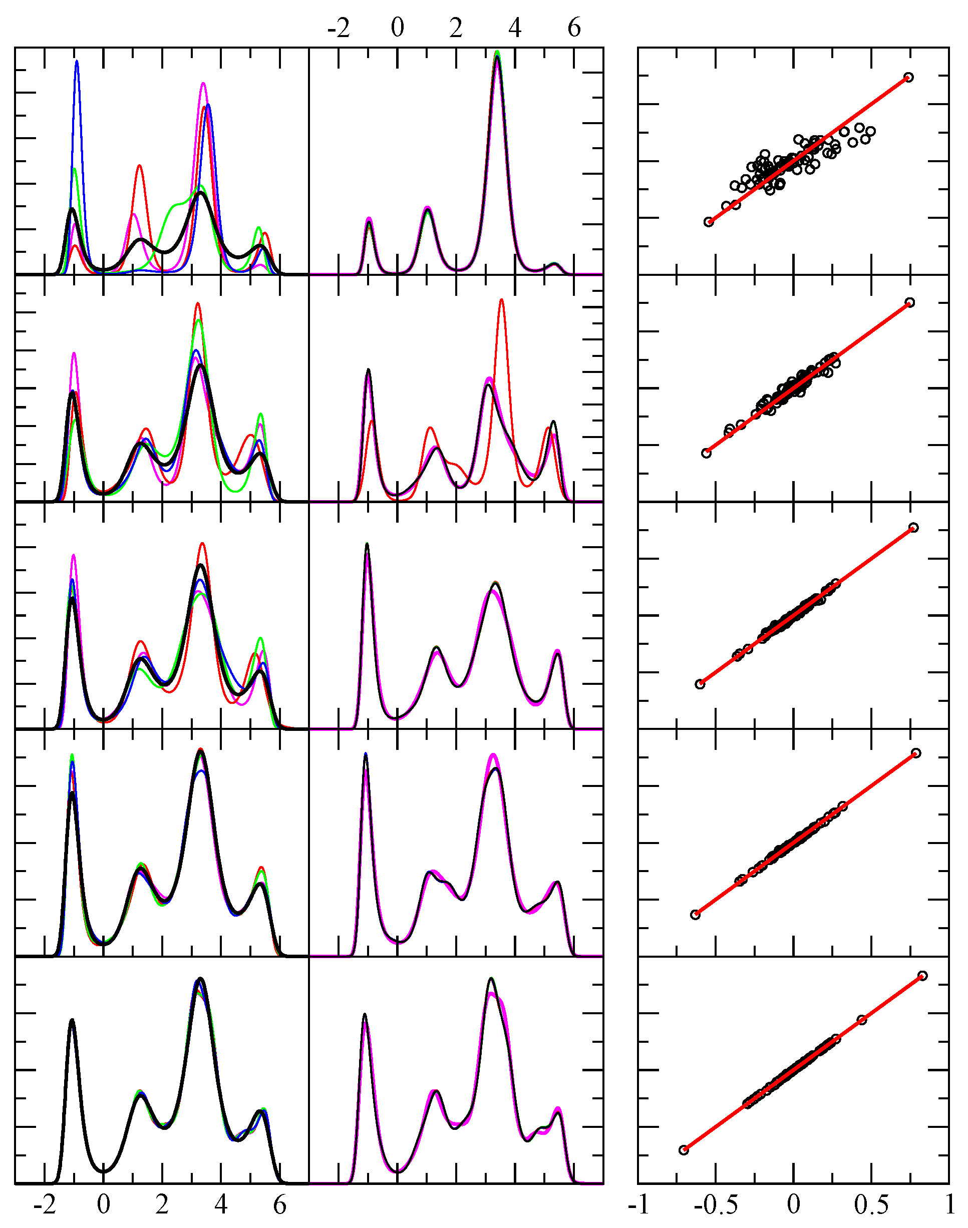
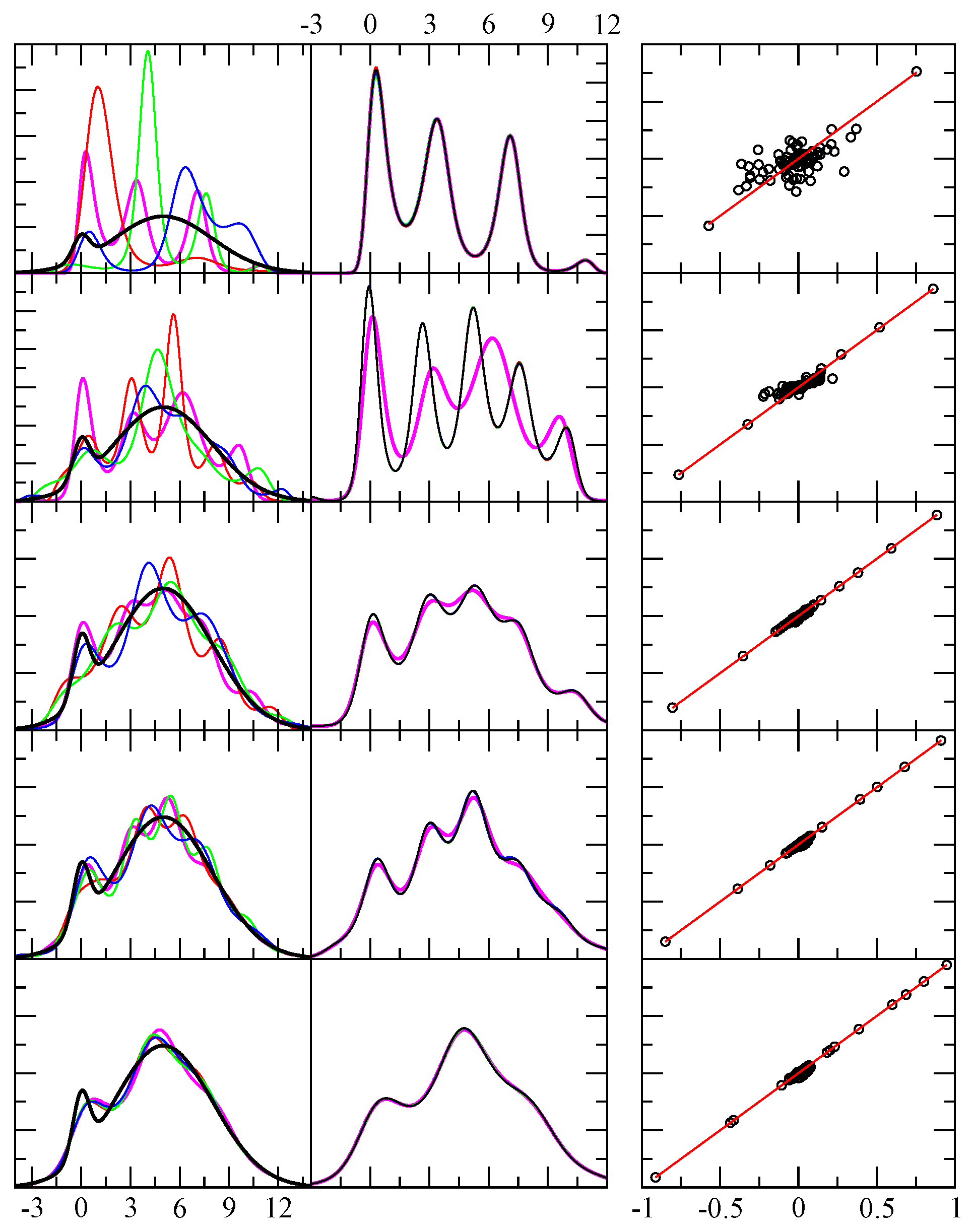
was determined by the normalization condition numerically (not selected). The parameters given here were simply adjusted by hand to give a distribution that showed four well-defined peaks of varying heights, widths and separations. Other than obtaining an interesting example, nothing special was associated with the selection of these parameters. The results are shown in
Figure 1 corresponding to four different test sets, each independently generated, for
,
,
,
number of samples. It is noted that for the case of
samples (having the least noise) one might expect the method will return a predicted
that will converge to the actual function given in Equation 17. However, it is found that for
samples, the optimal solutions for the least squares error typically contain between 33 to 35 coefficients. This indicates that there are many functions that look very close to
but not equal, and consisting of a lot more terms (33 versus 9). This result implies
is not a relevant target function, because the regions of
that do not lead to appreciable probability density are not well characterized as there are many ways to force the exponential toward zero. As such, there is a family of
that can yield regions of low probability, while maintaining the same values in regions of high probability. Rather than
, the relevant quantities are the level-function moments, such that the theoretical predicted values match well with the empirical values, while maximizing the entropy. In other words, there are indeed an infinite number of different
that will yield virtually indistinguishable results for
, and thus, indistinguishable results for
.
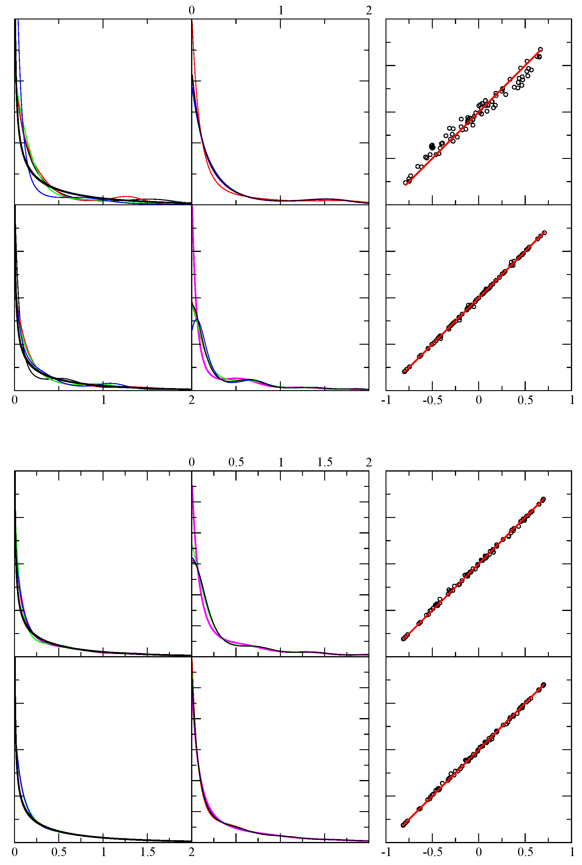
Figure 1.
Example results for test case 1. The first column shows the exact pdf (black) and four predicted pdf (red, green, blue, magenta) using independent random samples. The x-axis displays the range of the random variable in arbitrary units, while the y-axis is dimensionless. From top to bottom rows the number of random events in each sample were 64, 256, 1024, 4096 and 1048576. The second column is similar to the first, except it shows the result shown in magenta in the first column, and compares it with four additional results for the same sample — but from a different funnel diffusion run (black, red, green and blue). The third column shows 80 different level function moments calculated from the empirical data (x-axis) and from the theoretical prediction (y-axis) as defined in Equation 5. Perfect agreement would fall along the red line ().
3.2. Test example 2
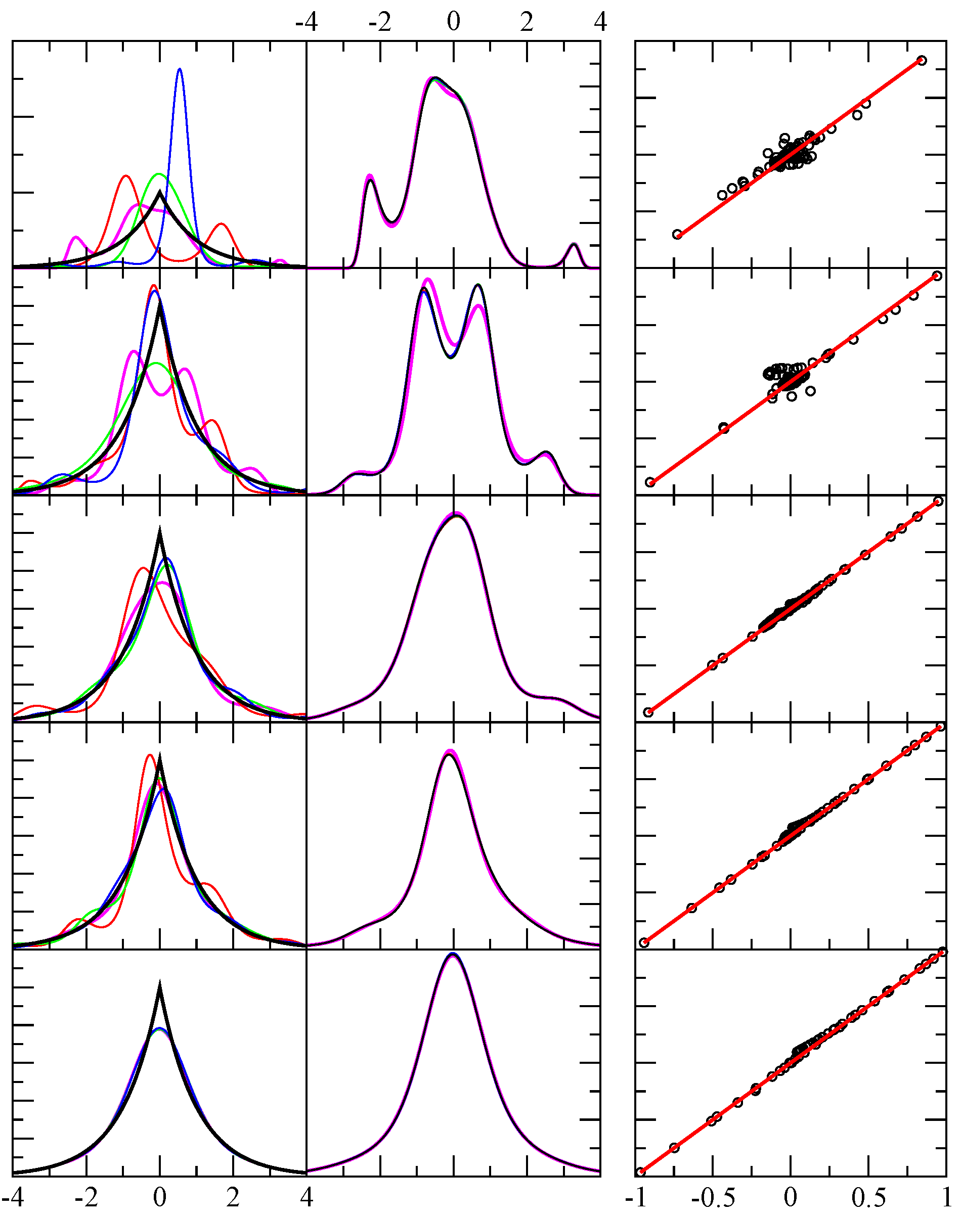
The pdf for test example 2 is defined as:
This pdf is a continuous function, but it has a cusp at
due to the discontinuous first derivative. The results for this example is shown in
Figure 2. Since the function
is continuously differentiable to all orders of
m, it is clear that an exact solution is impossible to achieve. Nevertheless, the method will always return a solution with smallest least squares error. For this exponential form, the wings for
are matched well, but the cusp is rounded. It might be expected that greater accuracy will be achieved by including more Chebyshev polynomials (
i.e., greater m). Specifically, the cusp will be better approximated. In principle this is true, but more samples are required for such a strategy to be successful.
Figure 2.
Example results for test case 2. The first column shows the exact pdf (black) and four predicted pdf (red, green, blue, magenta) using independent random samples. The x-axis displays the range of the random variable in arbitrary units, while the y-axis is dimensionless. From top to bottom rows the number of random events in each sample were 64, 256, 1024, 4096 and 1048576. The second column is similar to the first, except it shows the result shown in magenta in the first column, and compares it with four additional results for the same sample — but from a different funnel diffusion run (black, red, green and blue). The third column shows 80 different level function moments calculated from the empirical data (x-axis) and from the theoretical prediction (y-axis) as defined in Eqaution Equation 5. Perfect agreement would fall along the red line ().
Employing additional orthogonal polynomials (large m) beyond a point for which the data cannot justify m free parameters yields an undesirable, but interesting result (not shown). The result is that the sampled data will be effectively clustered by the appearance of many sharp peaks in the pdf, and outside of these peaks, the pdf is essentially zero. In other words, the result approaches a simple sum over Dirac-delta functions. The level-function moments will still yield good comparisons, because essentially this result is approximating a Gauss quadrature! The location of the sharp peaks are the quadrature points, and the area under their curves is the Gauss quadrature weight factors for the particular pdf. Thus, arbitrarily adding more Chebyshev polynomials should not be done. The algorithm that starts with using , then , and so forth will eventually yield a least squares error that is sufficiently small to terminate exploring greater m, or the least squares error will begin to increase. As such, in practice it is easy to avoid using too many Chebyshev polynomials. A consequence of this, however, is that if the pdf of interest has a sharp feature, such as a cusp, it should be expected that these type of features will be lost. On the other hand, this rounding effect is a natural smoothing of the pdf.
3.3. Test example 3
The pdf for test example 3 is defined as:
In this example,
C is determined numerically to satisfy the normalization condition. This particular functional form was motivated by an actual application to a physical system, related to the density of states for a one-dimensional harmonic oscillator combined with a relative Boltzmann factor. The important point here, is that the minimum value of
was known in advance (zero energy state of the system), and there is a divergence as
. Therefore, in these calculations, the finite left boundary condition was applied. The results are shown in
Figure 3. The 64 sample case is not shown in order to show the results of the other sample sizes more clearly. It is seen the method has absolutely no problem in representing this
, as given by Equation 19.
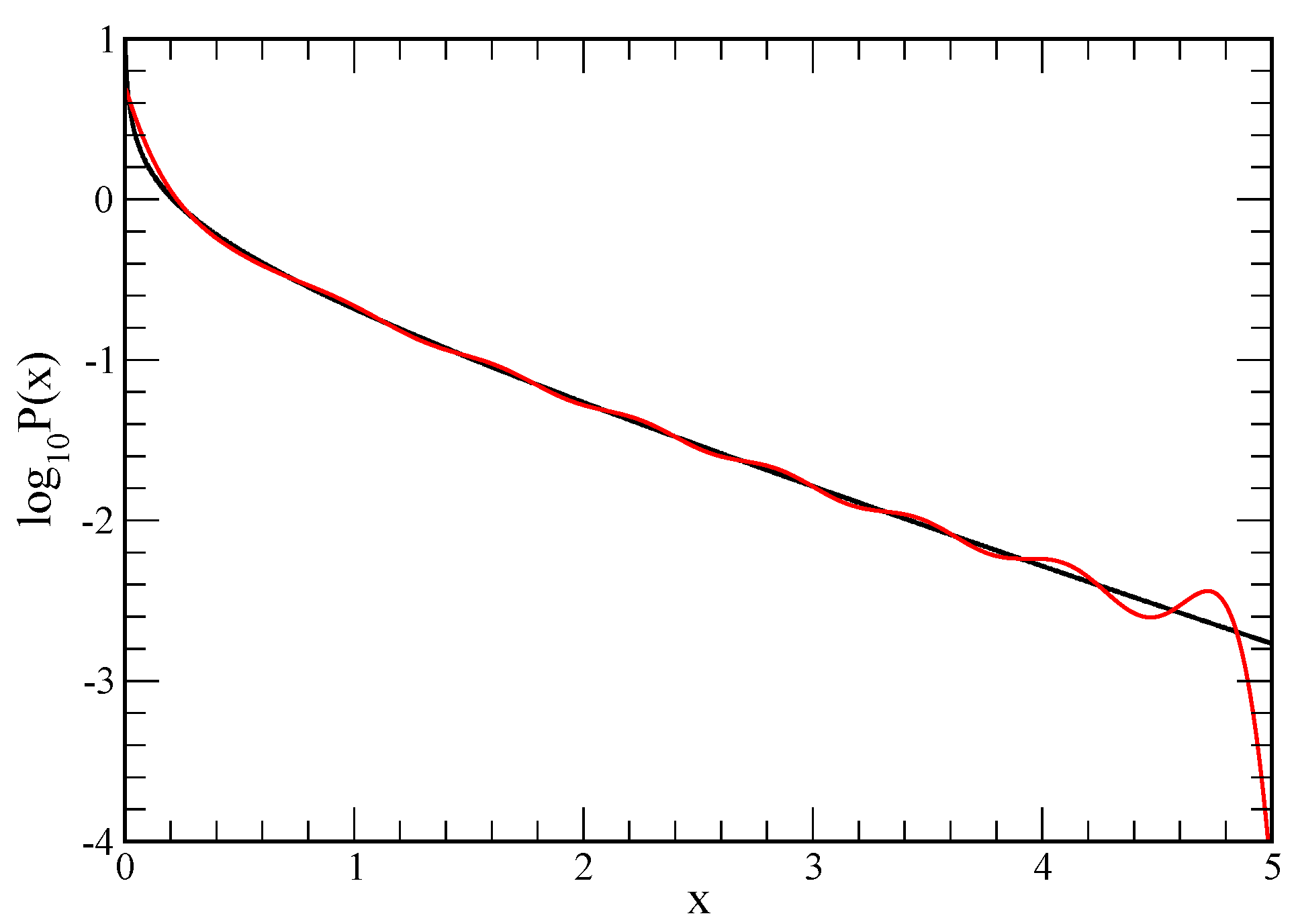
For the largest random data set consisting of
samples, the predicted
matches extremely well to the exact result. To show the level of deviation, the same data is plotted in
Figure 4 on a log scale for the probability. It is seen that the predicted
on the far tail starts to fall off much faster than the true
, which is mainly due to the Jacobian factor in transforming back from
to
. In this large sample case, the number of terms used is between 23 and 26. An important aspect of this method, is that for 1024 samples, there already emerges a very good representative of the true pdf.
3.4. Test example 4
The pdf for test example 4 is defined as:
Here,
denotes a Gaussian pdf of mean,
μ, and standard deviation,
σ. By construction, the functional form given in Equation 20 cannot be represented by a single exponential, which places the method outside of its range of applicability. Of course, in real applications this is not a priori known. Although the relative weighting of each Gaussian distribution, and the parameters of each Gaussian was arbitrarily selected, this case will provide insight into the following important question that needs to be answered. Will blindly using the method as described above provide a reasonable analytical form for
based on the maximum entropy assumption, albeit this assumption does not mimic the true pdf?
The results are given in
Figure 5, and the reconstruction of
is fair. In this case, even as the number of samples goes to
there is a fundamental discrepancy between the actual pdf and the predicted one. Nevertheless, the comparison between level-function moments are good enough for practical use. It is worth noting that the entropy of the predicted pdf is greater than the actual pdf as a consequence of trying to maximize it. In this case, the result cannot be improved because the entropy is being maximized under the constraints enforced by the various level-function moments. Because many of these level-functions are being used, the method still yields a good representation of the true pdf. For relatively small samples, it would be virtually impossible to distinguish the example 1 with say four Gaussian distributions. The final output of this method will allow a check on overall errors with respect to the level-function comparisons. As such, one can make an informed choice as to whether apply the predicted
or flag the calculation for further analysis.
Figure 3.
Example results for test case 3. Top panel: The first column shows the exact pdf (black) and four predicted pdf (red, green, blue, magenta) using independent random samples. The x-axis displays the range of the random variable in arbitrary units, while the y-axis is dimensionless. The top and bottom rows respectively show the results using 256 and 1024 random events. The second column is similar to the first, except it shows the result shown in magenta in the first column, and compares it with four additional results for the same sample — but from a different funnel diffusion run (black, red, green and blue). The third column shows 80 different level function moments calculated from the empirical data (x-axis) and from the theoretical prediction (y-axis) as defined in Eqaution 5. Perfect agreement would fall along the red line (). Bottom panel: The same description as the top panel, except that the number of events sampled in the top and bottom rows are respectively 4096 and 1048576.
![]()
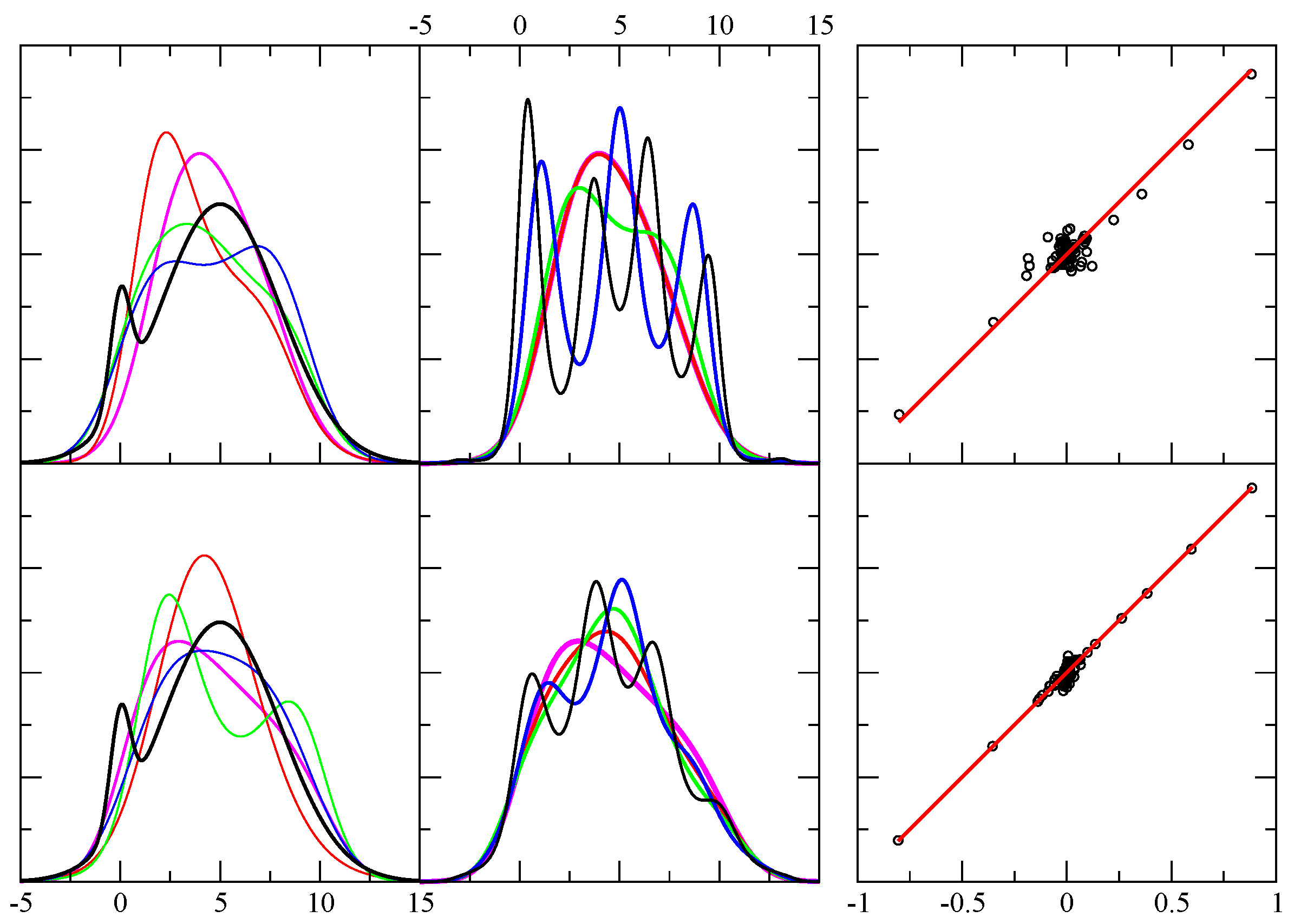
For this example test function, smoothing was also applied with results shown in
Figure 6. In practice, one may get a lot of oscillations in the pdf, especially when using small number of random samples. Since the noise in the data will be the main reason for these oscillations, the additional smoothing criteria is a viable option. It is seen that the agreement between empirical and theoretical level-function moments is worsened somewhat, compared to no smoothing. However, at the level of accuracy one can expect from using a small number of random samples in the first place, the increase in error is insignificant. The user through trial-and-error and inspection can try different smoothing levels to determine the best compromise between accuracy and smoothness. Note that the smoother the curves, the number of Chebyshev polynomials used to represent
decreases. This process is always subjective, because the smoothing is never required for the method to reproduce the input sample statistics. The only sure way to get a better estimate of the pdf is to collect more samples.
Figure 4.
Example results for test case 3. This re-plots one of the results from
Figure 3 that was shown as magenta for the 1048576 random samples. Here, we can see the accuracy better using a semi-log scale.
Figure 4.
Example results for test case 3. This re-plots one of the results from
Figure 3 that was shown as magenta for the 1048576 random samples. Here, we can see the accuracy better using a semi-log scale.
4. Discussion
The novel MEM described above has been applied to many application problems that initially motivated its development. In these applications, the true pdf is unknown. Nevertheless, the quantitative comparison between empirical and predicted moments consistently returns a satisfactory pdf, and these results will be published elsewhere in relation to the application of protein thermodynamics. In the last section, four example cases were considered to illustrate the results in a general context involving different types of known probability densities, all of which have a challenging aspect. Comparison of the predictions obtained by the new MEM for varying amounts of sampled data to the true pdf suggests that the “best” pdf under the maximum entropy assumption is indeed obtained. That is, the final predicted faithfully gives back what is known from the sampled data, and extrapolation is stable. Moreover, the results show constant improvement in converging toward a final pdf that is close (or the same) as the true pdf as the number of samples progressively increases. The success of this approach is not based on newly discovered principles about MEM. Rather, combining several novel steps has produced a robust MEM for generic applications.
Figure 5.
Example results for test case 4. The first column shows the exact pdf (black) and four predicted pdf (red, green, blue, magenta) using independent random samples. The x-axis displays the range of the random variable in arbitrary units, while the y-axis is dimensionless. From top to bottom rows the number of random events in each sample were 64, 256, 1024, 4096 and 1048576. The second column is similar to the first, except it shows the result shown in magenta in the first column, and compares it with four additional results for the same sample — but from a different funnel diffusion run (black, red, green and blue). The third column shows 80 different level function moments calculated from the empirical data (x-axis) and from the theoretical prediction (y-axis) as defined in Equation 5. Perfect agreement would fall along the red line ().
The most important aspect is to use many different level-function moments, some of which reflect the histogram (frequency counts). The level-function moments provide superior target functions, compared to elementary power moments, because taken together they give a much more uniform representation of all regions of the pdf. Consequently, this balanced characterization of the pdf makes the prediction for its analytical form robust. It is likely that the MEM formulated strictly as a Hausdorff moment problem would not yield a solution to any of the four cases considered here due to numerical instability [
4,
5,
6,
7,
16]. In addition to the advantages offered by using a multitude of level-function moments, the method developed here avoids using the Hessian matrix, uses an expansion in terms of orthogonal polynomials, and attempts to satisfy all the constraints using least squares error. It is worth noting that initially all the level-function moments were weighted equally. It was found, however, that the empirical moments associated with lower powers of
y are themselves more accurate. Employing an exponentially decreasing weight factor renders the decision of how many moments to keep a mute point, since adding more moments will have less and less effect until they become irrelevant. An improvement will be made in future work, such that the rate of decay in the exponent will be dependent on the number of random samples used in the analysis.
Figure 6.
Example results using smoothing on test case 4. The first column shows the exact pdf (black) and four predicted pdf (red, green, blue, magenta) using smoothing level, , (defined in Equation 16 and each case is drawn from independent random samples. The x-axis displays the range of the random variable in arbitrary units, while the y-axis is dimensionless. The top and bottom rows contain 256 and 1024 random events. The second column is similar to the first, except it shows the result shown in magenta in the first column, and compares it with four additional results for the same sample — but using different smoothing requests with shown as (black, blue, green, red). Note that the red curve is essentially indistinguishable from the curve shown in magenta. Of course, since the objective function changes, this implies a different funnel diffusion run as well. The third column shows 80 different level function moments calculated from the empirical data (x-axis) and from the theoretical prediction (y-axis) as defined in Equation 5. These results correspond to the smoothing case shown in the first column by the magenta curve. Perfect agreement would fall along the red line ().
![]()
The method automates the least squares minimization to stop at a reasonable cutoff, so as not to over-interpret the data. Tuning these criteria was based on applying the method to several applications. As mentioned above, including more Chebyshev polynomials can often continue to reduce the least squares error, but the resulting pdf begins to follow clustering in the data, which is most likely noise. Too close of an agreement with the actual data is over-fitting, because the uncertainty in the data itself scales as
, and the best resolution in the estimate of probability scales as
. As such, attempting to exactly fit to the data makes no sense, and it is better to use only the number of Chebyshev polynomials that can be justified based on the number of samples on hand. The following heuristic for termination in exploring greater number of terms is given by:
was found to work well. When the
reaches 1 the pdf already results in an excellent reconstruction of
for all test cases. Although lowering the
cutoff may be advantageous, it was unnecessary for the applications of interest that motivated this work. No attempt was made to optimize based on each problem of interest. For example, the number of bins used to represent the histograms of the y-variables and x-variables could adjust based on the nature of the statistics. Unequal binning could be incorporated, and different weights could be applied to the level-functions. Many technical improvements could be made, and work in this direction is in progress. When finished, the expectation is to release a freeware general application tool.
The strengths of the current method is that it is robust, where variation in different solutions for predicted is much lower than the variation that one gets due to noise when using a finite number of random samples (when the number is lower than 1000). The fact that different estimates are obtained for different independent samples is not a weakness. Limiting the number of samples is effectively adding noise to the true pdf, because a finite number of samples create feature perturbations due to fluctuations. This approach eliminates the need to add auxiliary noise, but more importantly it provides insight into the performance characteristics of determining the true pdf from limited samples. Unless something is a priori known about the form of the pdf, the sampled data must drive the representative prediction of . In this context, the funnel diffusion approach is an excellent method to determine the expansion coefficients, which are related to the Lagrange multipliers. Multiple solutions from independent funnel diffusion runs yield insignificant deviations in the predicted compared to the variation found in due to limited samples (noise). For a case where m reaches 40 (sequentially trying 1 to 40) the funnel diffusion typically takes less than 20 minutes on a 2.3 GHz computer. Replacing the sequential search with a bisection method will reduce the calculation time to just a few minutes. The funnel diffusion method has been applied to many different optimization problems, and has always provided a robust self-adapting simulated annealing method. In particular, it self determines the degree of randomness needed as the annealing takes place. In standard simulated annealing, the degree of randomness is controlled by temperature. In many applications, such as the one considered here (i.e., minimizing a function) temperature is an artificial concept. Funnel diffusion is conceptually more natural, and its implementation is embarrassing simple.
The weakness of the presented MEM derives only from the maximum entropy assumption itself. In particular, the maximum entropy assumption need not be true for the actual data. Demanding maximum entropy is basically an automatic smoother, since the broadest possible pdf consistent with the level-function moments will be generated. As such, another improvement is currently under development that separately applies the MEM into distinct modes. Each mode will separately be subject to the maximum entropy assumption, but multiple modes will be considered. In a similar way that the number of terms in the function is optimized (smallest m that describes the data well), this generalization finds the least number of modes that describes the data well. The form and procedure of the k-th mode is identical to this method, since it is a method based on one mode. The number of terms for the k different functions will be . Then the estimate for the pdf is given as where is the statistical weight of the k-th mode, and is calculated using the current method. This generalization is being implemented into a general user-friendly application tool (to be published).

