1. Introduction
Evidence from climate science suggests that, in at least some cases, the dynamics of planetary atmospheres obey a principle of maximum entropy production [
1,
2,
3]. The rates of heat flow in these systems are such that either increasing or decreasing them by a significant amount would reduce the rate at which entropy is produced within the system. If this principle could be extended to some more general class of physical systems then it would have a wide range of important implications.
However, the principle as currently formulated suffers from an important conceptual problem, which I term the system boundary problem: it makes different predictions depending on where one draws the boundaries of the system. In this paper I present a new argument based on Edwin Jaynes’ approach to statistical mechanics, which I believe can give a constructive answer to this problem.
If the maximum entropy production principle (MEPP) turns out to be a general property of physical systems under some yet-to-be-determined set of conditions then it could potentially have a huge impact on the way science can deal with far-from-equilibrium systems. This is because planetary atmospheres are extremely complex systems, containing a great number of processes that interact in many ways, but the MEPP allows predictions to be made about them using little information other than knowledge of the boundary conditions. If this trick can be applied to other complex far-from-equilibrium physical systems then we would have a general way to make predictions about complex systems’ overall behaviour. The possibility of applying this principle to ecosystems is particularly exciting. Currently there is no widely accepted theoretical justification for the MEPP, although some significant work has been carried out by Dewar [
4,
5] and other authors [
6,
7,
8,
9].
However, maximising a system’s entropy production with respect to some parameter will in general give different results depending on which processes are included in the system. In order for the MEPP to make good predictions about the Earth’s atmosphere one must include the entropy produced by heat transport in the atmosphere but not the entropy produced by the absorption of incoming solar radiation [
10]. Any successful theoretical derivation of the MEPP must therefore provide us with a procedure that tells us which system we should apply it to. Without this the principle itself is insufficiently well defined. In
Section 2 of this paper I present an overview of the principle, emphasising the general nature of this problem.
Like the work of Dewar [
4,
5], the approach I wish to present is based on Jaynes’ [
11,
12,
13,
14,
15,
16,
17] information-theory based approach to statistical mechanics, which is summarised in
Section 3. Briefly, Jaynes’ argument is that if we want to make our best predictions about a system we should maximise the entropy of a probability distribution over its possible states subject to knowledge constraints, because that gives a probability distribution that contains no “information” (i.e., assumptions) other than what we actually know. Jaynes was able to re-derive a great number of known results from equilibrium and non-equilibrium thermodynamics from this single procedure.
In
Section 3.1. I argue that if we want to make predictions about a system at time
(in the future), but we only have knowledge of the system at time
, plus some incomplete knowledge about its kinetics, Jaynes’ procedure says we should maximise the entropy of the system’s state at time
. This corresponds to maximising the entropy produced between
and
. No steady state assumption is needed in order to make this argument, and so this approach suggests that the MEPP may be applicable to transient behaviour as well as to systems in a steady state.
This simple argument does not in itself solve the system boundary problem, because it only applies to isolated systems. The Solar system as a whole can be considered an isolated system, but a planetary atmosphere cannot. However, in
Section 4. I present a tentative argument that there is an additional constraint that must be taken account of when dealing with systems like planetary atmospheres, and that when this is done we obtain the MEPP as used in climate science. If this argument is correct then the reason we must exclude the absorption of radiation when using MEPP to make predictions about planetary atmospheres is not because there is anything special about the absorption of radiation, but because the dynamics of the atmosphere would be the same if the heat were supplied by some other mechanism.
The maximum entropy production principle, if valid, will greatly affect the way we conceptualise the relationship between thermodynamics and kinetics. There is also a pressing need for experimental studies of the MEPP phenomenon. I will comment on these issues in
Section 5.
The main arguments of this paper are in sections
Section 3.1. and
Section 4. Readers familiar with the background material may wish to start there.
2. Background: The Maximum Entropy Production Principle and Some Open Problems
The Maximum Entropy Production Principle (MEPP), at least as used in climate science, was first hypothesised by Paltridge [
2], who was looking for an extremum principle that could be used to make predictions about the rates of heat flow in the Earth’s atmosphere in a low resolution (10 box) model. Paltridge tried several different such principles [
18] before discovering that adjusting the flows so as to maximise the rate of production of entropy within the atmosphere gave impressively accurate reproductions of the actual data. The MEPP was therefore an empirical discovery. It has retained that status ever since, lacking a well-accepted theoretical justification, although some significant progress has been made by Dewar [
4,
5], whose work we will discuss shortly.
The lack of a theoretical justification makes it unclear under which circumstances the principle can be applied in atmospheric science, and to what extent it can be generalised to systems other than planetary atmospheres. The aim of this paper is to provide some steps towards a theoretical basis for the MEPP which may be able to answer these questions.
2.1. An Example: Two-Box Atmospheric Models
A greatly simplified version of Paltridge’s model has been applied to the atmospheres of Mars and Titan in addition to Earth by Lorenz, Lunine and Withers [
3]. The authors state that the method probably also applies to Venus. It is worth explaining a version of this simple two-box version of the MEPP model, because it makes clear the form of the principle and its possible generalisations. Readers already familiar with such models may safely skip to
Section 2.2.
The model I will describe differs from that given in [
3], but only in relatively minor details. Lorenz et al. use a linear approximation to determine the rate of heat loss due to radiation, whereas I will use the non-linear function given by the Stefan-Boltzmann law. This is also done in Dewar’s version of the model in [
4].
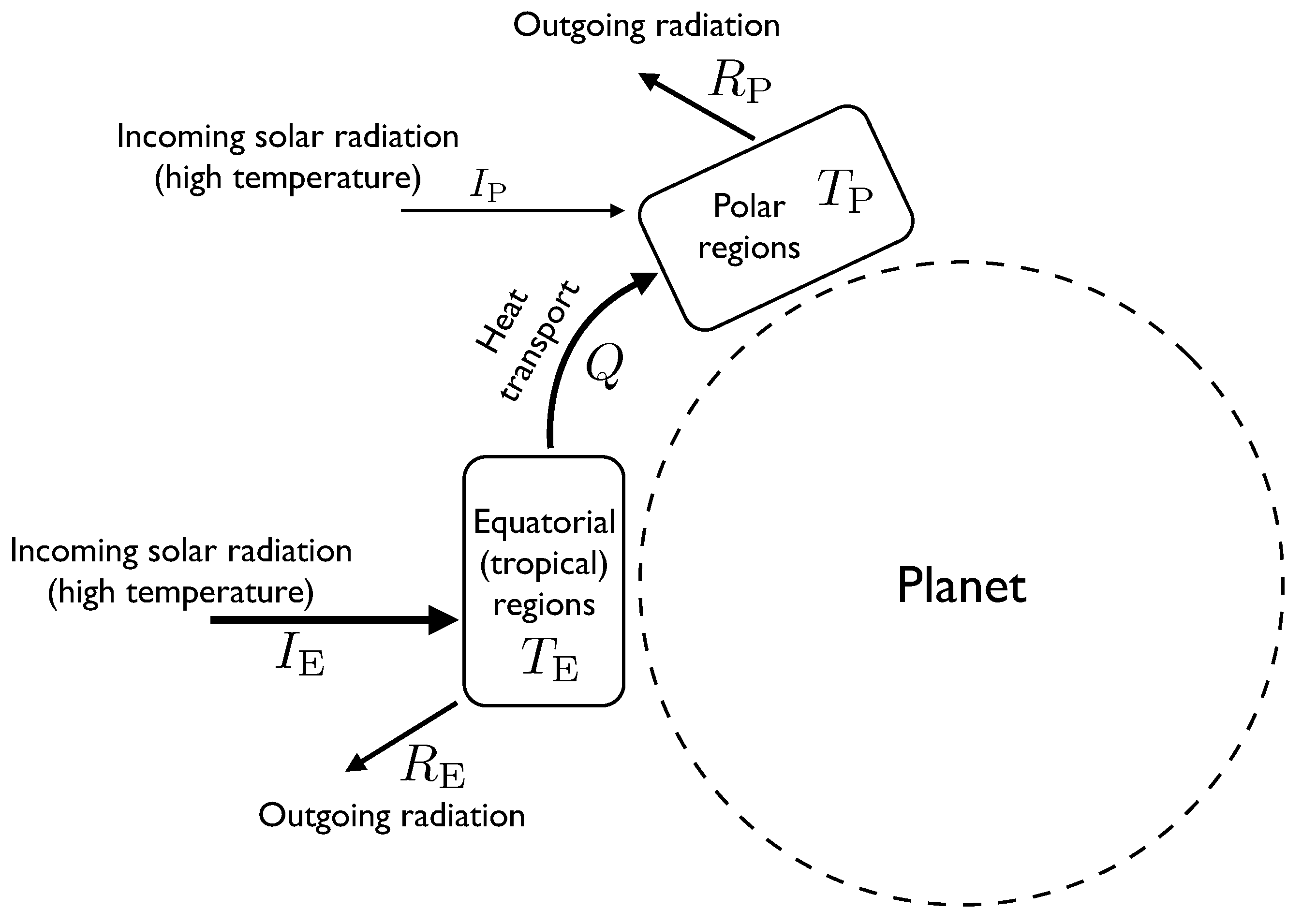
In these models, the atmosphere is divided into two boxes of roughly equal surface area, one representing the equatorial and tropical regions, the other representing the temperate and polar regions (see
Figure 1). Energy can be thought of as flowing between the boxes, mostly by convection, and each box can be very roughly approximated as having a single temperature.
Figure 1.
A diagram showing the components of the two-box atmospheric heat transport model. Labels written next to arrows indicate rates of flow of energy, whereas labels in boxes represent temperature.
Figure 1.
A diagram showing the components of the two-box atmospheric heat transport model. Labels written next to arrows indicate rates of flow of energy, whereas labels in boxes represent temperature.
Energy flows into the equatorial region at a rate . This represents the flux of incoming solar radiation (insolation). This radiation is effectively at the same temperature as the sun, which is about 5700 K. The atmospheric system is assumed in this model to be in a steady state, so this incoming energy must be balanced by outgoing flows. One outgoing flow is caused by the equatorial region radiating heat to space. The rate at which this occurs depends on the temperature of the equatorial region and is approximately determined by the Stefan-Boltzmann law, which says that the outgoing radiative flux is proportional to . The other outflow from the equatorial region is the heat flow Q transported by atmospheric processes to the polar region. We will treat Q as a parameter of the model. We will eventually use the MEPP to estimate the value of Q.
Putting this together, we have the energy balance equation for the equatorial region , where k is a parameter whose value depends on the surface area of the equatorial region and on the Stefan-Boltzmann constant. For a given value of Q, this can be solved to find . Larger values of Q result in a lower temperature for the equatorial region.
Similarly, for the polar region we have . is smaller than because the polar regions are at an angle to the incoming radiation, which is why the heat flow Q from the equator to the poles is positive.
We now wish to calculate the rate of entropy production due to the atmospheric heat transport. This is given by the rate at which the heat flow
Q increases the entropy of the polar region, minus the rate at which
Q decreases the entropy of the tropical region. Entropy is heat divided by temperature, so the rate of entropy production due to
Q is given by
or
. The quantity
will be referred to as the
gradient.
Solving the steady state energy balance equations for
and
we obtain the entropy production as a function of
Q:
The exact form of this equation is not important, but it has some important properties. when . At this point the gradient is large, but the heat flow is zero. The inverse temperature difference decreases with increasing heat flow, so that is also zero when . At this value of Q the temperatures of the equator and the poles are equal, and so there is no entropy production because there is no change in temperature of the energy being transferred. A value of Q greater than this would imply that the temperature of the poles must be greater than that of the equator, and the entropy production would become negative. An external source of energy would thus be required to maintain such a flow, and so can be thought of as the maximum value for Q. The observed value for Q in real atmospheres is somewhere between these two extremes.
The value of reaches a peak at some value of Q between 0 and . (Numerically, it looks to be about .) The work of Lorenz et al. essentially consists finding the value of Q which produces this maximum for models parameterised to match the physical situations of the atmospheres of Earth, Mars and Titan. This produces good predictions of the rate of atmospheric heat transport for these three bodies, which provides good empirical support for the MEPP.
2.2. Generalisation: Negative Feedback Boundary Conditions
The two-box atmospheric model described above has an interesting and important feature: the presence of what I will call negative feedback boundary conditions. By this I mean that if one thinks of the system as including the convective transport processes in the atmosphere, but not the emission and absorption of radiation, then the dependence of the temperature gradient on the flow rate can be thought of as a constraint imposed on the system from outside.
Usually in non-equilibrium thermodynamics we would consider one of two different types of boundary condition: we could impose a constant gradient upon the system (corresponding to holding
and
constant), and ask what would be the resulting rate of flow; or else we could hold the flow rate constant and ask the value of the gradient. The boundary conditions on the atmospheric heat transport in the two box model are a generalisation of this, whereby neither the temperature gradient nor the heat flow rate are held constant, but instead the gradient is constrained to be a particular function of the flow. The situation in Paltridge’s original 10 box model is more complicated, with more variables and more constraints, but in either case the result is an underspecified system in which many different steady state rates of flow are possible, each with a different associated value for the temperature gradient. As emphasised by Dewar [
4,
5], the MEPP is properly seen as a principle that we can use to select from among many possible steady states in systems that are underspecified in this way.
I use the term “negative feedback boundary conditions” to emphasise that, in situations analogous to these two-box atmospheric models, the gradient is a decreasing function of the flow, which results in a unique maximum value for the entropy production, which occurs when the flow is somewhere between its minimum and maximum possible values.
The notion of gradient can readily be extended to systems where the flow is of something other than heat. In electronics, the flow is the current I and the gradient is , the potential difference divided by temperature (the need to divide by temperature can be seen intuitively by noting that has the units of entropy). For a chemical process that converts a set of reactants X to products Y, the flow is the reaction rate and the gradient is , where and are the chemical potentials of X and Y.
If the effectiveness of the two-box model is the result of a genuine physical principle, one might hope that it could be extended in general to some large class of systems under negative feedback constraints. This might include the large class of ecological situations noted by Odum and Pinkerton [
19], which would provide a much-needed tool for making predictions about complex ecological systems. Odum and Pinkerton’s hypothesis was that processes in ecosystems occur at a rate such that the rate at which work can be extracted from the system’s environment is maximised. If one assumes that all this work eventually degrades into heat, as it must in the steady state, and that the temperature of the environment is independent of the rate in question, then this hypothesis is equivalent to the MEPP.
The MEPP cannot apply universally to all systems under negative feedback boundary conditions. As a counter-example, we can imagine placing a resistor in an electrical circuit with the property that the voltage it applies across the resistor is some specific decreasing function of the current that flows through it. In this case we would not expect to find that the current was such as to maximise the entropy production. Instead it would depend on the resistor’s resistance R. The constraint that , plus the imposed relationship between V and I, completely determines the result, with no room for the additional MEPP principle.
For this reason, the MEPP is usually thought of as applying only to systems that are in some sense complex, having many “degrees of freedom” [
3], which allow the system to in some way choose between many possible values for the steady state flow. A successful theoretical derivation of the MEPP must make this idea precise, so that one can determine whether a given system is of the kind that allows the MEPP to be applied.
In Dewar’s approach, as well as in the approach presented in the present paper, this issue is resolved by considering the MEPP to be a predictive principle, akin to the second law in equilibrium thermodynamics: the entropy production is always maximised, but subject to constraints. In equilibrium thermodynamics the entropy is maximised subject to constraints that are usually formed by conservation laws. In Dewar’s theory, the entropy production is maximised subject to constraints formed instead by the system’s kinetics. If we make a prediction using the MEPP which turns out to be wrong, then this simply tells us that the constraints we took into account when doing the calculation were not the only ones acting on the system. Often, in systems like the resistor, the kinetic constraints are so severe that they completely determine the behaviour of the system, so that there is no need to apply the MEPP at all.
An interesting consequence of this point of view is that, in the degenerate case of boundary conditions where the gradient is fixed, the MEPP becomes a maximum flow principle. With these boundary conditions the entropy production is proportional to the rate of flow, and so according to the MEPP, the flow will be maximised, subject to whatever macroscopic constraints act upon it. Likewise, for a constant flow, the MEPP gives a prediction of maximal gradient.
However, there is another serious problem which must be solved before a proper theory of maximum entropy production can be formulated, which is that the principle makes non-trivially different predictions depending on where the system boundary is drawn. In the next two sections I will explain this problem, and argue that Dewar’s approach does not solve it.
2.3. The System Boundary Problem
A substantial criticism of MEPP models in climate science is that of Essex [
10], who pointed out that the entropy production calculated in such models does not include entropy produced due to the absorption of the incoming solar radiation. This is important because maximising the total entropy production, including that produced by absorption of high-frequency photons, gives a different value for the rate of atmospheric heat transport, one that does not agree with empirical measurements. This will be shown below.
This is a serious problem for the MEPP in general. It seems that we must choose the correct system in order to apply the principle, and if we choose wrongly then we will get an incorrect answer. However, there is at present no theory which can tell us which is the correct system.
We can see this problem in action by extending the two-box model to include entropy production due to the absorption of radiation. The incoming solar radiation has an effective temperature of K. When this energy is absorbed by the equatorial part of the atmosphere its temperature drops to (or if it is absorbed at the poles), of the order 300 K. The entropy production associated with this drop in temperature is given by , making a total rate of entropy production . No entropy is produced by the emission of radiation, since the effective temperature of thermal radiation is equal to the temperature of the body emitting it. The outgoing radiation remains at this temperature as it propagates into deep space. (Though over very long time scales, if it is not absorbed by another body, its effective temperature will be gradually be reduced by the expansion of space.)
As in
Section 2.1. we can substitute the expressions for
and
to find
as a function of
Q. A little calculation shows that its maximum occurs at
, which is the maximum possible value for
Q, corresponding to a state in which the heat flow is so fast that the temperatures of the tropical and polar regions become equal. This is a different prediction for
Q than that made by maximising
. Indeed, for this value of
Q,
becomes zero.
Thus the results we obtain from applying the MEPP to the Earth system depend on where we draw the boundary. If we draw the system’s boundary so as to include the atmosphere’s heat transport but not the radiative effects then we obtain a prediction that matches the real data, but if we draw the boundary further out, so that we are considering a system that includes the Earth’s surrounding radiation field as well as the Earth itself, then we obtain an incorrect (and somewhat physically implausible) answer.
This problem is not specific to the Earth system. In general, when applying the MEPP we must choose a specific bounded region of space to call the system, and the choice we make will affect the predictions we obtain by using the principle. If the MEPP is to be applied to more general systems we need some general method of determining where the system boundary must be drawn.
2.4. Some Comments on Dewar’s Approach
Several authors have recently addressed the theoretical justification of the MEPP [
4,
5,
7,
8,
9], see [
6] for a review. Each of these authors takes a different approach, and so it is fair to say there is currently no widely accepted theoretical justification for the principle.
The approach presented here most closely resembles that of Dewar [
4,
5]. Dewar’s work builds upon Edwin Jaynes’ maximum entropy interpretation of thermodynamics [
11,
12]. Jaynes’ approach, discussed below, is to look at thermodynamics as a special case of a general form of Bayesian reasoning, the principle of maximum entropy (
MaxEnt, not to be confused with the maximum entropy production principle).
Dewar offers two separate derivations of the MEPP from Jaynes’ MaxEnt principle, one in [
4] and the other in [
5]. Both derive from Jaynes’ formalism, which is probably the fundamentally correct approach to non-equilibrium statistical mechanics.
Unfortunately I have never been able to follow a crucial step in Dewar’s argument (equations 11–14 in [
4]), which shows that a particular quantity is equal to the entropy production. It is difficult to criticise an argument from the position of not understanding it, but it seems that both of Dewar’s derivations suffer from two important drawbacks. Firstly, they both rely on approximations whose applicability is not clearly spelled out, and secondly neither offers a satisfactory answer to the question of how to determine the appropriate system boundary.
In [
4], Dewar writes that his derivation tells us which entropy should be maximised: the material entropy production, excluding the radiative components, which are to be treated as an imposed constraint. But there seems to be nothing in the maths which implies this. Indeed, in [
5] the principle is presented as so general as to apply to all systems with reversible microscopic laws—which is to say, all known physical systems—and this condition clearly applies as much to the extended earth system, with the surrounding radiation field included, as it does to the atmosphere alone. Dewar’s approach therefore does not solve the system boundary problem and cannot apply universally to all systems, since this would give rise to contradictory results. Dewar’s derivations may well be largely correct, but there is still a piece missing from the puzzle.
In the following sections I will outline a new approach to the MEPP which I believe may be able to avoid these problems. Although not yet formal, this new approach has an intuitively reasonable interpretation, and may be able to give a constructive answer to the system boundary problem.
3. Thermodynamics as Maximum Entropy Inference
Both Dewar’s approach and the approach I wish to present here build upon the work of Edwin Jaynes. One of Jaynes’ major achievements was to take the foundations of statistical mechanics, laid down by Boltzmann and Gibbs, and put them on a secure logical footing based on Bayesian probability and information theory [
11,
12,
13,
14,
15,
16,
17].
On one level this is just a piece of conceptual tidying up: it could be seen as simply representing a different justification of the Boltzmann distribution, thereafter changing the mathematics of statistical mechanics very little, except perhaps to express it in a more elegant form. However, on another level it can be seen as unifying a great number of results in equilibrium and non-equilibrium statistical mechanics, putting them on a common theoretical footing. In this respect Jaynes’ work should, in the present author’s opinion, rank among the great unifying theories of century physics. It also gives us a powerful logical tool — maximum entropy inference — that has many uses outside of physics. Most importantly for our purposes, it frees us from the near-equilibrium assumptions that are usually used to derive Boltzmann-type distributions, allowing us to apply the basic methodology of maximising entropy subject to constraints to systems arbitrarily far from thermal equilibrium.
Jaynes gives full descriptions of his technique in [
11,
12], with further discussion in [
13,
14,
15,
16,
17]. I will present a very brief overview of Jaynes’ framework, in order to introduce the arguments in the next section.
Like all approaches to statistical mechanics, Jaynes’ is concerned with a probability distribution over the possible microscopic states of a physical system. However, in Jaynes’ approach we always consider this to be an “epistemic” or Bayesian probability distribution: it does not necessarily represent the amount of time the system spends in each state, but is instead used to represent our state of knowledge about the microstate, given the measurements we are able to take. This knowledge is usually very limited: in the case of a gas in a chamber, our knowledge consists of the macroscopic quantities that we can measure—volume, pressure, etc. These values put constraints on the possible arrangements of the positions and velocities of the molecules in the box, but the number of possible arrangements compatible with these constraints is still enormous.
The probability distribution over the microstates is constructed by choosing the distribution with the greatest entropy , while remaining compatible with these constraints. This is easy to justify: changing the probability distribution in a way that reduces the entropy by n bits corresponds to making n bits of additional assumptions about which microscopic state the system might be in. Maximising the entropy subject to constraints formed by our knowledge creates a distribution that, in a formal sense, encodes this knowledge but no additional unnecessary assumptions.
Having done this, we can then use the probability distribution to make predictions about the system (for example, by finding the expected value of some quantity that we did not measure originally). There is nothing that guarantees that these predictions will be confirmed by further measurement. If they are not then it follows that our original measurements did not give us enough knowledge to predict the result of the additional measurement, and there is therefore a further constraint that must be taken into account when maximising the entropy. Only in the case where sufficient constraints have been taken into account to make good predictions of all the quantities we can measure should we expect the probability distribution to correspond to the fraction of time the system spends in each state.
In thermodynamics, the constraints that the entropy being maximised is subject to usually take the form of known expectation values for conserved quantities. For example, the quantities in question might be internal energy and volume. We will denote the energy and volume of the
state by
and
, and their expectations by
U and
V. Maximising the entropy subject to these constraints gives rise to the probability distribution
where
Z is a normalisation factor known as the partition function, and
are parameters whose value can in principle be calculated from the constraints if all the values
and
are known.
and
are closely related the the “intensive” quantities of thermodynamics, since it can be shown that
, where
is Boltzmann’s constant, and
. This can be extended naturally to other conserved quantities, such as mole number or electric charge, giving rise to parameters that relate to chemical potential or voltage, etc. An enormous number of previously known results from equilibrium and non-equilibrium thermodynamics can be derived quite directly from the properties of this distribution.
This method can be extended to deal with a continuum of states rather than a set of discrete ones. This introduces some extra subtleties (see [
17, chapter 12], [
20]) but does not change the overall picture. In this paper we will assume that the possible microstates of physical systems are discrete, with the understanding that the arguments presented here are unlikely to change substantially in the continuous limit.
There is a subtle point regarding the status of the second law in Jaynes’ interpretation of thermodynamics [
13]. Liouville’s theorem states that, if one follows every point in a distribution of points in a system’s microscopic phase space over a period of time, the entropy of this distribution does not change. However, if we make macroscopic measurements of the system at the end of this time period we will in general get different results. If the results of these new measurements are sufficient to predict the system’s macroscopic behaviour in the future then we are justified in re-maximising the entropy subject to constraints formed by the new measurements. This new re-maximised entropy cannot be less than the entropy at the beginning of the time period by Liouville’s theorem, but it can be greater. This increase in entropy corresponds to a loss of information, which in this case occurs because, although we have some specific information about the system’s past macroscopic state, this information is no longer useful to us in predicting the system’s future states, so we can disregard it.
3.1. A New Argument for the MEPP
Once Jaynes’ approach to thermodynamics is understood, the argument I wish to present for the MEPP is so simple as to be almost trivial. However, there are some aspects to it which have proven difficult to formalise, and hence it must be seen as a somewhat tentative sketch of what the true proof might look like.
Jaynes’ argument tells us that to make the best possible predictions about a physical system, we must use the probability distribution over the system’s microstates that has the maximum possible entropy while remaining compatible with any macroscopic knowledge we have of the system. Now let us suppose that we want to make predictions about the properties of a physical system at time , in the future. Our knowledge of the system consists of measurements made at the present time, , and some possibly incomplete knowledge of the system’s kinetics.
The application of Jaynes’ procedure in this case seems conceptually quite straight-forward: we maximise the entropy of the system we want to make predictions about—the system at time —subject to constraints formed by the knowledge we have about it. These constraints now include not only the values of conserved quantities but also restrictions on how the system can change over time.
If the system in question is isolated then it cannot export entropy to its surroundings. In this case, if we consider the entropy at time to be a fixed function of the constraints then maximising the entropy at corresponds to maximising the rate at which entropy is produced between and . Note that no steady state assumption is required to justify this procedure.
This appears to show that, for isolated systems at least, maximum entropy production is a simple corollary of the maximum entropy principle. However, it should be noted that the entropy which we maximise at time
is not necessarily equal to the thermodynamic entropy at
as usually defined. Let us denote by
the entropy of the probability distribution over the system’s microstates at time
t, when maximised subject to constraints formed by measurements made at time
, together with our knowledge about the system’s microscopic evolution. Jaynes called this quantity the caliber [
16]. In contrast, let
to denote the thermodynamic entropy at time
t, which is usually thought of as the information entropy when maximised subject to constraints formed by measurements made at time
t only. Then
, but
can be less than
. In particular, if we have complete knowledge of the microscopic dynamics then
by Liouville’s theorem, which always applies to the microscopic dynamics of an isolated physical system, even if the system is far from thermodynamic equilibrium.
The procedure thus obtained consists of maximising the thermodynamic entropy subject to constraints acting on the system not only at the present time but also in the past. Our knowledge of system’s kinetics also acts as a constraint when performing such a calculation. This is important because in general systems take some time to respond to a change in their surroundings. In this approach this is dealt with by including our knowledge of the relaxation time among the constraints we apply when maximising the entropy.
There is therefore a principle that could be called “maximum entropy production” which can be derived from Jaynes’ approach to thermodynamics, but it remains to be shown in which, if any, circumstances it corresponds to maximising the thermodynamic entropy. From this point on I will assume that for large macroscopic systems, and can be considered approximately equal, so that maximising the thermodynamic entropy at time yields the same results as maximising the information entropy. The validity of this step remains to be shown.
This suggests that applying Jaynes’ procedure to make predictions about the future properties of a system yields a principle of maximum production of thermodynamic entropy: it says that the best predictions about the behaviour of isolated systems can be made by assuming that the approach to equilibrium takes place as rapidly as possible. However it should be noted that this argument does not solve the system boundary problem in the way that we might like, since it applies only to isolated systems. The heat transport in the Earth’s atmosphere is not an isolated system, but the Solar system as a whole is, to a reasonable approximation. Thus this argument seems to suggest unambiguously that the MEPP should be applied to the whole Solar system and not to Earth’s atmosphere alone — but this gives incorrect predictions, as shown in
Section 2.3. A tentative solution to this problem will be discussed in
Section 4.
3.2. Application to the Steady State with a Fixed Gradient
In this section I will demonstrate the application of this technique in the special case of a system with fixed boundary conditions. I will use a technique similar to the one described by Jaynes in [
15], whereby a system which could be arbitrarily far from equilibrium is coupled to a number of systems which are in states close to equilibrium, allowing the rate of entropy production to be calculated. In
Section 4. I will extend this result to the more general case of negative feedback boundary conditions.
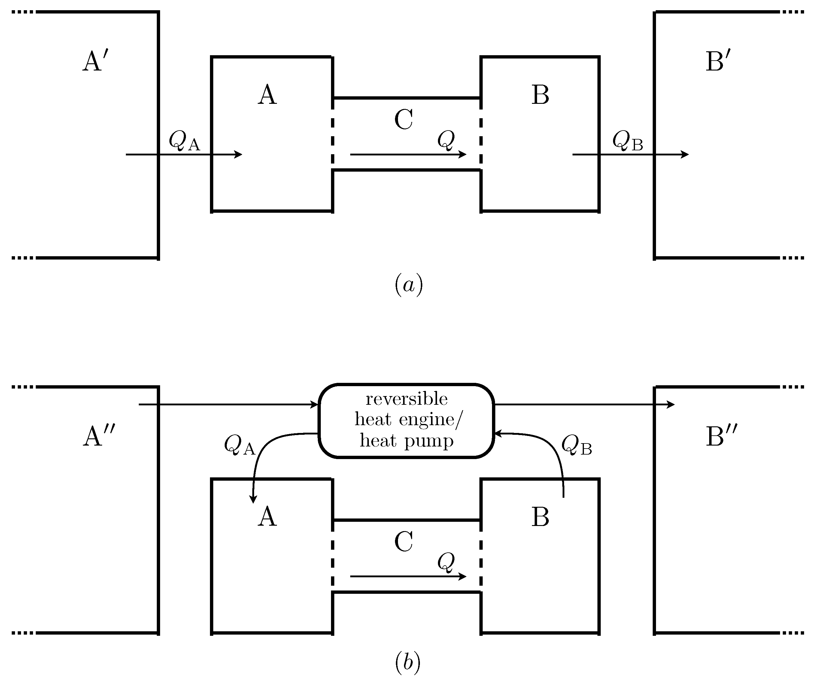
Consider a system consisting of two large heat baths and , coupled by another system that can transfer energy between them, about which we have some limited knowledge. Our assumption will be that and are relatively close to thermodynamic equilibrium, so that it makes sense to characterise them as having definite temperatures and internal energies . This need not be the case for , which could be arbitrarily complex and involve many interacting far-from-equilibrium processes. The only assumption we will make about is that it can be considered to be in a steady state on the time scale under consideration.
We will consider the evolution of the system over a time period from some arbitrary time to another time . We will assume the duration of this time period to be such that the temperatures of and do not change appreciably.
At a given time t, the (maximised) information entropy of the whole system, denoted , is given by the thermodynamic entropy of the reservoirs, , plus the entropy of . By “the entropy of ” we mean in this context the entropy of a probability distribution over the possible microstates of , when maximised subject to all knowledge we have about the kinetics of , together with the boundary conditions of constant and . Since is potentially a very complex system this may be difficult if not impossible to calculate. However, the steady state assumption implies that our knowledge of the system is independent of time. Maximising the entropy of a probability distribution over ’s microstates should give us the same result at as it does for . The entropy of is thus constant over time.
We now treat our knowledge of the state of the system (including the reservoirs) at time
as fixed. We wish to make a maximum entropy prediction of the system’s state at time
, given this knowledge. Since
is fixed, maximising
is equivalent to maximising
where
Q is the steady state rate of heat transport from
to
. Since
and
are fixed, this corresponds to maximising
Q subject to whatever constraints our knowledge of
’s kinetics puts upon it. We have therefore recovered a maximum flow principle from Jaynes’ maximum entropy principle.
This reasoning goes through in exactly the same way if the flow is of some other conserved quantity rather than energy. It can also be carried out for multiple flows, where the constraints can include trade-offs between the different steady-state flow rates. In this case the quantity which must be maximised is the steady state rate of entropy production. This is less general than the MEPP as used in climate science, however, since this argument assumed fixed gradient boundary conditions.
4. A Possible Solution to the System Boundary Problem
The argument presented in
Section 3.1. does not in itself solve the System Boundary Problem in a way which justifies the MEPP as it is used in climate science. Instead, it seems to show that only the entropy production of isolated systems is maximised, in the sense that the approach to equilibrium happens as rapidly as possible, subject to kinetic constraints. Planetary atmospheres are not isolated systems, but the Solar system as a whole is, to a reasonable degree of approximation, so it seems at first sight that we should maximise the total entropy production of the Solar system in order to make the best predictions. As shown in
Section 2.3., this results in a prediction of maximum heat flow, rather than maximum entropy production, for planetary atmospheres.
It could be that this reasoning is simply correct, and that there is just something special about planetary atmospheres which happens to make their rates of heat flow match the predictions of the MEPP. However, in this section I will try to argue that there is an extra constraint that must be taken into account when performing this procedure on systems with negative feedback boundary conditions. This constraint arises from the observation that the system’s behaviour should be invariant with respect to certain details of its environment. I will argue that when this constraint is taken account of, we do indeed end up with something that is equivalent to the MEPP as applied in climate science.
We now wish to apply the argument described in
Section 3.1. to a situation analogous to the two-box atmosphere model. Consider, then, a system consisting of two finite heat reservoirs,
and
, coupled by an arbitrarily complex sub-system
that can transport heat between them. This time the reservoirs are to be considered small enough that their temperatures can change over the time scale considered. The system as a whole is not to be considered isolated, but instead each reservoir is subjected to an external process which heats or cools it at a rate that depends only on its temperature (this is, of course, an abstraction of the two-box atmospheric model). Let
and
stand for the temperatures of the two reservoirs and
Q be the rate of the process of heat transport from
to
. Let
be the rate of heat flow from an external source into
, and
be the rate of heat flow from
B into an external sink. In the case of negative feedback boundary conditions,
is a decreasing function and
increasing.
Suppose that our knowledge of this system consists of the functions and , together with the conservation of energy, and nothing else: we wish to make the best possible predictions about the rate of heat flow Q without taking into account any specific knowledge of the system’s internal kinetics. As in Jaynes’ procedure, this prediction is not guaranteed to be correct. If it is then it should imply that the sub-system responsible for the heat transport is so under-constrained that information about the boundary conditions is all that is needed to predict the transport rate.
We cannot directly apply the procedure from
Section 3.1. because this system is not isolated. We must therefore postulate a larger system to which the system
is coupled, and treat the extended system as isolated. However, there is some ambiguity as to how this can be done: there are many different extended systems that would produce the same boundary conditions on
. In general entropy will be produced in the extended system as well as inside
, and the way in which the total entropy production varies with
Q will depend on the precise configuration of the extended system.
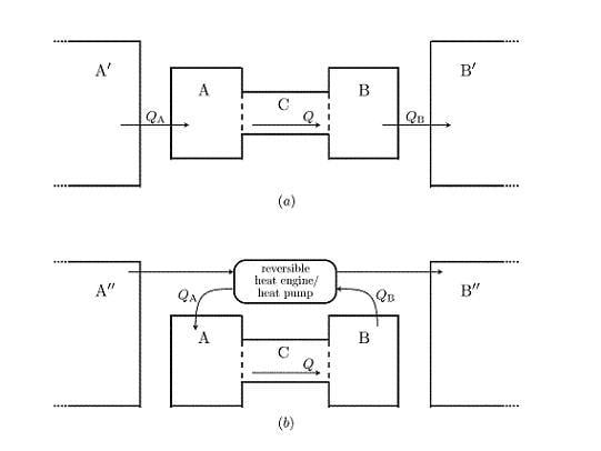
Figure 2 shows two examples of possible extended systems. The first is somewhat analogous to the real situation of the Earth’s atmosphere. Heat flows into
from a much larger reservoir of constant temperature
, which is roughly analogous the the solar radiation field, and out of
into a large reservoir
, which can be thought of as representing deep space. The second law implies that the temperature of
must be greater than the maximum possible temperature of
, and that of
must be less than
’s minimum temperature. This in turn means that entropy is produced when heat is transferred from
to
and from
to
. In this scenario, the total entropy production is maximised when
Q is maximised.
Figure 2.
Two possible ways in which negative feedback boundary conditions could be realised. Heat flows into from a much larger reservoir , and out of into another large reservoir . A reversible heat engine is used to extract power by transferring heat between two external reservoirs and , and this power is used to transfer heat reversibly out of and into . In this version the only entropy produced is that produced inside due to the heat flow Q.
Figure 2 shows another, more complicated possibility. In this scenario the functions
and
are the same, but the flows are caused by a different mechanism. A heat engine extracts work from the temperature gradient between two external reservoirs (now denoted
and
). This work is used by reversible heat pumps to extract heat from
and to add heat to
. This is done at a carefully controlled rate so that the rates of heat flow depend on the temperature of
and
in exactly the same way as in the other scenario.
Since all processes in this version of the external environment are reversible, the only entropy produced in the extended system is that due to Q, the heat flow across . The boundary conditions on are the same, but now the maximum in the total entropy production occurs when the entropy production within is maximised, at a value for Q somewhere between 0 and its maximum possible value.
Although the first of these scenarios seems quite natural and the second somewhat contrived, it seems odd that the MEPP should make different predictions for each of them. After all, their effect on the system is, by construction, identical. There is no way that system can “know” which of these possible extended systems is the case, and hence no plausible way in which its steady state rate of heat flow could depend on this factor. This observation can be made even more striking by noting that one could construct an extended system for which the total entropy production is maximised for any given value of Q, simply by connecting a device which measures the temperatures of and and, if they are at the appropriate temperatures, triggers some arbitrary process that produces entropy at a high rate, but which does not have any effect upon .
Clearly an extra principle is needed when applying the MEPP to systems of this type: the rate of heat flow Q should be independent of processes outside of the system which cannot affect it. This can be thought of as an additional piece of knowledge we have about the extended system, which induces an additional constraint upon the probability distribution over its microstates.
The question now is how to take account of such a constraint when maximising the entropy. It seems that the solution must be to maximise the information entropy of a probability distribution over all possible states of the extended system, subject to knowledge of the system , the functions and , and nothing else. We must ignore any knowledge we may have of processes taking place outside of , and , because we know that those processes cannot affect the operation of .
But this again presents us with a problem that can be solved by maximising an entropy. We know that outside the system there is another system, which we might collectively call , which is capable of supplying a constant flow of energy over a long period of time. But this is all we know about it (or at least, we are deliberately ignoring any other knowledge we may have about it). Jaynes’ principle tells us that, if we want to make the minimal necessary set of assumptions, we should treat it as though its entropy is maximised subject to constraints formed by this knowledge.
Let us consider again at the two scenarios depicted in
Figure 2. In the first, the temperature of
is constrained by the second law to be substantially higher than that of
. If
is to cause a flow of
K units of energy through system
, its entropy must increase by at least
, an amount substantially greater than the entropy produced inside
. The total entropy of
is of the order
, where
and
are the (very large) internal energies of
and
.
The situation in the second scenario is different. In this case the temperatures of and can be made arbitrarily close to one another. This suggests that in some sense, the entropy of the external environment, which is of the order , can be higher than in the other scenario. (The machinery required to apply the flow reversibly will presumably have a complex structure, and hence a low entropy. But the size of machinery required does not scale with the amount of energy to be supplied, so we may assume that the size of this term is negligible compared to the entropy of the reservoirs.) In this scenario, if K units of energy are to flow through (assumed for the moment to be in the steady state), the entropy of need only increase by , which is precisely the amount of entropy that is produced inside .
I now wish to claim that, if we maximise the entropy of , we end up with something which behaves like the second of these scenarios, supplying a flow of heat through reversibly. To see this, start by assuming, somewhat arbitrarily, that we know the volume, composition and internal energy of , but nothing else. Equilibrium thermodynamics can then (in principle) be used to tell us the macroscopic state of in the usual way, by maximising the entropy subject to these constraints. Let us denote the entropy thus obtained by .
But we now wish to add one more constraint to , which is that it is capable of supplying a flow of energy through over a given time period. Suppose that the total amount of entropy exported from during this time period is s (this does not depend on the configuration of , by assumption). The constraint on , then, is that it is capable of absorbing those s units of entropy. Its entropy must therefore be at most . Again there will be another negative term due to the configurational entropy of any machine required to actually transport energy to and from , but this should become negligible for large s.
Maximising the entropy of a large environment
subject to the boundary conditions of
over a long time scale thus gives an entropy of
. But if
has an entropy of
then it cannot produce any additional entropy in supplying the flow of heat through
, because the only entropy it is capable of absorbing is the entropy produced inside
. Therefore, if we maximise the entropy of
subject to these constraints we must end up with an environment which behaves like the one shown in
Figure 2, supplying the flow of energy reversibly.
This will be true no matter which constraints we initially chose for the volume, internal energy and composition of , so we can now disregard those constraints and claim that in general, if all we know about is that it is capable of supplying a flow of energy through , we should assume that it does so reversibly, producing no additional entropy as it does so. This is essentially because the vast majority of possible environments capable of supplying such a heat flow do so all-but-reversibly.
This result gives us the procedure we need if we want to maximise the total entropy production of the whole system (), subject to knowledge only of and its boundary conditions, disregarding any prior knowledge of . In this case we should assume that there is no additional contribution to the entropy production due to processes in , and thus count only the entropy production due to the heat flow across .
Therefore, completing the procedure described in
Section 3.1. subject to the constraint of the invariance of
with respect to the details of
, we obtain the result that the best possible predictions about
should be made by maximising the entropy production of
alone. This procedure should be followed even if we have definite
a priori knowledge about the rate of entropy production in
, as long as we are sure that the details of
should not affect the rate of entropy production in
.
4.1. Application to Atmospheres and Other Systems
In this section I have presented a very tentative argument for a way in which the system boundary problem might be resolved. If this turns out the be the correct way to resolve the system boundary problem then its application to the Earth’s atmosphere is equivalent to a hypothesis that the atmosphere would behave in much the same way if heat were supplied to it reversibly rather than as the result of the absorption of high-temperature electromagnetic radiation. It is this invariance with respect to the way in which the boundary conditions are applied that singles the atmosphere out as the correct system to consider when applying MEPP. However, the argument could also be applied in reverse: the fact that the measured rate of heat flow matches the MEPP prediction in this case could be counted as empirical evidence that the atmosphere’s behaviour is independent of the way in which heat is supplied to it.
It is worth mentioning again that although I have presented this argument in terms of heat flows and temperature, it goes through in much the same way if these are replaced by other types of flow and their corresponding thermodynamic forces. Thus the argument sketched here, if correct, should apply quite generally, allowing the same reasoning to be applied to a very wide range of systems. The method is always to vary some unknown parameters so as to maximise the rate of entropy production of a system. The system should be chosen to be as inclusive as possible, while excluding any processes that cannot affect the parameters’ values.

