1. Introduction
The synchronization phenomenon is the subject of much work nowadays and attracts attention from various field of science, engineering, and social behavior [
1]. In particular, the coupling between dynamical systems is of particular interest as it can be encountered in a number of manners. To investigate the associated interactions involves the detection and quantification of the strength and direction (or asymmetry) of the pertinent couplings and major effort has revolved around the task of ascertaining directional couplings. Information-theoretic approaches become of importance in such respect. One of such treatments is of paramount interest for us here, related to the quantity called “transfer entropy” (TE) [
2], which can quantify statistical coherence among systems evolving in time. The corresponding approach was designed so as to overcome difficulties encountered using the standard time delayed mutual information, which exhibits problems in distinguishing between information that is actually exchanged from shared information due to common history and input signals [
3]. The TE ignores these influences by appropriately conditioning associated transition probabilities [
2]. One is thus able to distinguish effectively driving from responding elements and to detect asymmetry in the interaction of subsystems. Interesting progress is advanced in [
3] by estimating the transfer entropy by recourse to a symbolization-technique, tantamount to a sort of coarse graining that facilitates accessible manipulation. One then speaks of symbolic TE (STE) and finds that it is a robust and computationally fast method to quantify the dominating direction of information flow between time series from coupled systems.
In this work we apply the STE to the classical limit of quantum mechanics (CLQM) that, contrary to the widespread belief, remains an open problem since the problem of the emergence of classical mechanics from quantum mechanics is by no means solved. In spite of many results on the
asymptotics, it is not yet clear how to explain the classical motion of macroscopic bodies within the standard quantum mechanics. In this paper we shall analyze,
via the STE, a special case of evolution from quantum to classical behavior [
4] in the framework of a well-known semi-classical model that represents the interaction of matter with a given field [
5,
6].
2. The CLQM for a Special Semi-Classical Model
Since the introduction of the decoherence concept in the early 1980s by Zeh, Zurek, and other authors like Habib [
7,
8,
9,
10,
11], the emergence of the classical world from Quantum Mechanics has been a subject of much interest. Among the associated issues one can mention the emergence of classical dynamics, specially classical chaos, in quantum systems through continuous measurement by Habib, Bhattacharya, Ghose, and Jacobs, among others [
12,
13] and the “decoherent histories approach” by Gisin, Brun, Halliwell, and Percival [
14,
15,
16,
17]. Additionally, authors like Everitt, who explore the quantum-classical crossover in the behavior of a quantum field mode [
18] and the chaotic-like and non-chaotic-like behavior in nonlinear quantum systems [
19] are of certain interest. Also deserve mention Ralph [
20], Greenbaum [
21] and Lifshitz [
22].
Quite a bit of quantum insight is to be gained from semiclassical perspectives. Several methodologies are available (WKB, Born-Oppenheimer approach,
etc.). The model of References [
5,
6,
23] considers two interacting systems: one classical, the other quantal. This makes sense whenever the quantum effects of one of the two systems are negligible in comparison to those of the other one. Examples can be readily found. We can just mention Bloch equations [
24], two-level systems interacting with an electromagnetic field within a cavity [
25,
26,
27], collective nuclear motion [
28],
etc.
We have investigated the classical limit of a semiclassical model containing both classical and quantum degrees of freedom in Reference [
23]. In contrast to what was done in the above mentioned papers via a master equation for the density operator [
10,
11,
16], or by recourse to equivalent stochastic equations for pertinent expectation values [
12,
13], we consider a simplified scheme in which the interaction with the environment is simulated by classical variables. Here the classical limit is obtained whenever one satisfies the relation given by Equation (4) for the total energy and the invariant
I (see Equation (5)), related to the uncertainty principle.
Thus, we deal with a special bipartite system that represents the zero-th mode contribution of a strong external field to the production of charged meson pairs [
6,
23], whose Hamiltonian reads
where
i) and
are quantum operators,
ii) A and
classical canonical conjugate variables and
iii) is an interaction term that introduces nonlinearity,
being a frequency. The quantities
and
are masses, corresponding to the quantum and classical systems, respectively. As shown in Reference [
4], in dealing with Equation (
1) one faces an autonomous system of nonlinear coupled equations
where
. The system of Equation (2) follows immediately from Ehrenfest’s relations [
4]. To study the classical limit we also need to consider the classical counterpart of the Hamiltonian given by Equation (
1)
where all the variables are classical. Recourse to Hamilton’s equations allows one to find the classical version of Equation (2) (see Reference [
4] for further details). These equations are identical in form to Equation (2) after suitable replacement of quantum mean values by classical variables,
i.e.,
,
and
. The classical limit is obtained by letting the “relative energy”
where
E is the total energy of the system and
I is an invariant of the motion described by the system of equations previously introduced (Equation (2)), related to the Uncertainty Principle
A classical computation of
I yields
. Thus,
I vanishes when it is evaluated using the classical variables
A and
, for all
t,
i.e.,
, a fact that exhibits the self-consistency of our methodology. A measure of the degree of convergence between classical and quantum results in the limit of Equation (4) is given by the norm
of the vector
[
4]
where the three components vector
is the “quantum” part of the solution of the system defined by Equation (2) and
its classical counterpart.
A detailed study of this model, was performed in References [
4,
23]. The main results of these references, pertinent for our discussion, can be succinctly detailed as follows: in plotting diverse dynamical quantities as a function of
(as it grows from unity to
∞), one finds
an abrupt change in the system’s dynamics for a special value of , to be denoted by . From this value onwards, the pertinent dynamics starts converging to the classical one. It is thus possible to assert that
provides us with an
indicator of the presence of a quantum-classical “border”. The zone
corresponds to the semi-quantal regime investigated in Reference [
23]. This regime, in turn, is characterized by
two different sub-zones [
23]. One of them is an almost purely quantal one, in which the microscopic quantal oscillator is just slightly perturbed by the classical one, and the other section exhibits a transitional nature (semi-quantal). The border between these two sub-zones can be well characterized by a “signal” value
. A significant feature of this point resides in the fact that, for
,
chaos is always found. The relative number of chaotic orbits (with respect to the total number of orbits) grows with
and tends to unity for
[
23].
Thus, as
grows from
(the “pure quantum instance”) to
(the classical situation), a significant series of
morphology changes is detected, specially in the transition-zone (
). The concomitant orbits exhibit features that are not easily describable in terms of Equation (6), which is a
global measure of the degree of convergence in amplitude (of the signal). What one needs instead is
a statistical type of characterization, as that described in References [
29,
30,
31], involving the notions of entropy and statistical complexity. Both quantifiers can be evaluated in various ways as, for instance, by employing the wavelet approach (see References [
29,
30] and references therein) or the Bandt and Pompe method (see Reference [
31] and references therein). These two statistical quantifiers are able to adequately identify the properties of the three zones that enter the quantum-classical evolution (as
varies). However, the intermediate-transition zone needs still more detailed analysis that will be shown below to be provided by recourse to the symbolic transfer entropy.
3. Symbolic Transfer Entropy
In order to understand the flow of information between two different time series Schreiber [
2] introduced the transfer entropy concept. This quantifier allows to determine driving and responding elements and to detect asymmetry in the interaction between two systems. Let us consider
and
,
, two realizations of the systems
X and
Y. The transfer entropy, defined as the Kullback-Leibler entropy between the conditional probabilities
and
, measures the deviation from the generalized Markov property
This deviation quantifies the influence of the system
Y on
X. Observe that the transfer entropy is explicitly nonsymmetric under the changes of
and
. This tool has been applied for assessing causality relations in different fields like econophysics [
32,
33,
34] and chaotic communications [
35]. It was also shown that the Schreiber’s definition of TE coincides with the standard definition of the conditional mutual information [
36,
37].
Unfortunately, due to several drawbacks such as the high amount of data required and its sensitivity to noise contributions, this information theoretic measure is very hard to estimate in practical analyses. More recently, Staniek and Lehnertz [
3] proposed a modified version of the transfer entropy, the symbolic transfer entropy, based on the Bandt and Pompe symbolization technique [
38]. The new symbolic series are obtained by reordering the amplitude values of the original time series
and
. Consider the sequence of amplitude values associated to the time series
with embedding dimension
and time delay
τ given by
o each time
i we are assigning a
D-dimensional vector that results from the evaluation of the time series at times
. Clearly, the greater the
D value, the more information about the past is incorporated into the ensuing vectors. By the ordinal pattern of order
D related to the time
i we mean the permutation
of
defined by
In this way the vector defined by Equation (9) is converted into a unique symbol
. Further details about the Bandt and Pompe method can be found in References [
39,
40]. For all the
possible permutations
of order
D, their associated relative frequencies can be naturally computed by
where ♯ is the cardinality of the set—roughly speaking, the number of elements in it. Thus, a permutation probability distribution
is obtained from the time series
[
42]. Obviously the same can be done for
. Given these permutation probability distributions the symbolic transfer entropy (STE) is defined as
where the sum runs over all possible permutations and
δ denotes a time step. The joint probability
is the joint relative frequency of the three events
,
and
. The conditional probabilities
and
are given by
and
respectively. The symbolic transfer entropy
quantifies the flow of information from system
Y to
X.
is defined in the same way. Finally, the directionality index
allows us to determine the dominating direction of information flow between the two systems
X and
Y. If
,
X will be the driving system and
Y the responding one. On the other hand this quantifier will be negative for
Y driving
X.
4. Results
Remember that the CLQM-model we are dealing with here is represented by five non-linear coupled equations (Equation (2)). A correct reconstruction of the attractor associated with the integration of this system is achieved using an embedding dimension
. We will deal with vectors with components of
data-points each one, for each orbit. Notice that the condition
is satisfied. We take the time delay
as it is usually chosen [
38]. In obtaining our numerical results we chose
for the system’s parameters. For the initial conditions needed to tackle our system (Equation (2)) we took
,
i.e., we fixed
E and then varied
I so as to obtain our different
-values. Additionally, we set
,
(both in the quantum and the classical instances), and
taking values in the interval
, with
. The data-points used to evaluate the probability distribution
p in Equation (12) are given by both, the solutions of Equation (2) and its classical counterpart. Finally, a time step
was used in our calculations.
We will here choose
X, in Equation (12), as representing the series of values pertaining to a quantum system’s variable, while
Y does the same classically.
Figure 1 and
Figure 2 display the quantities
,
and
vs.
, taking
and
. Instead, in
Figure 3 we have
and
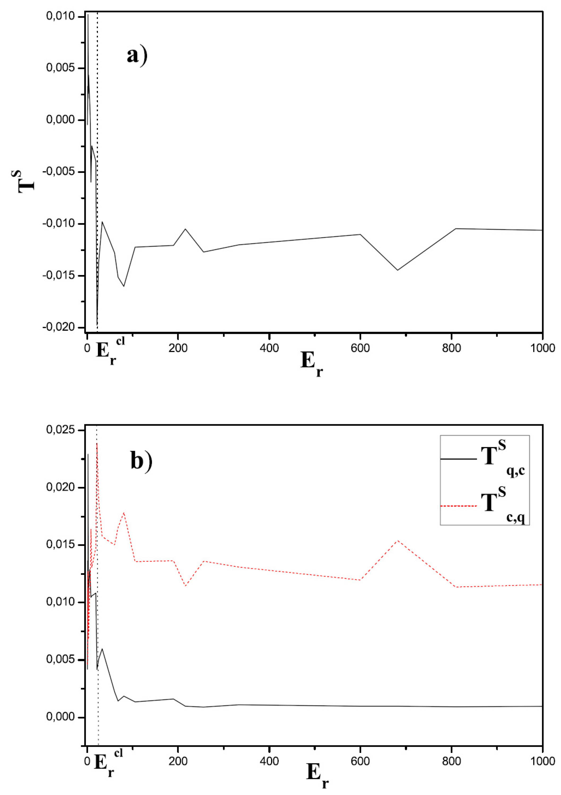
. Similar results ensue if other pairs of quantum-classical variables are selected, that are not shown on space-saving grounds.
We pass now to consider what happens when
varies moving leftward from
. In the fully classical case (
),
“lead” [
43] the remaining variables of the system of classical equations
. For large
’s (
but small) the classical variables
“still dominate” and lead the quantal
ones. See
Figure 1 for the
scenario. This plot, and also
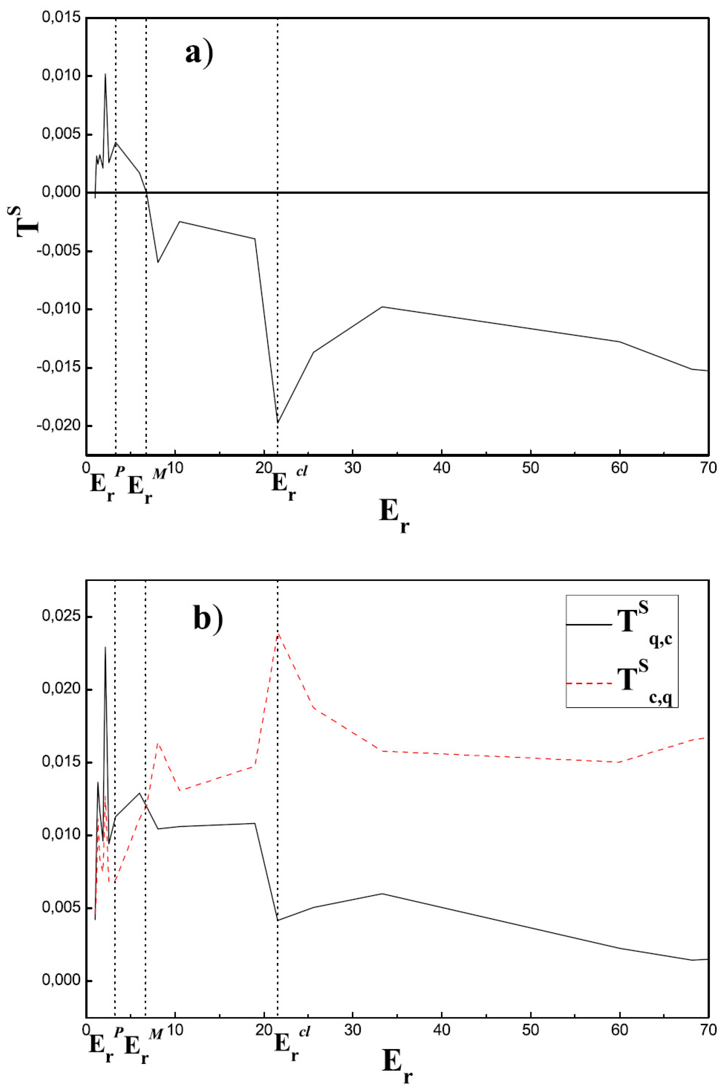
Figure 2, are representative of our process. As
diminishes further and reaches the particular value
where
(
Figure 2), the behavior changes. From then on, the quantum mean value
begins to dominate. As
decreases (or
I grows) the influence of the Uncertainty Principle becomes stronger, thus we conclude that it is the responsible for the change. At
the Uncertainty Principle becomes important enough and the quantum variable suddenly begins to drive the process (
Figure 2). It dominates until, for
, we again get
. This last result is to be expected, since for
the quantum system acquires all the energy
and the classical one gets located at the fixed point
[
23]. Since
the two system become decoupled and no information flows between them. Note in
Figure 2b) that
and
practically vanish. Small biases are obtained due to finite-sample effects. If we increase the series’ size these errors diminish. Anyway, if
,
and no error is found in
[
3].
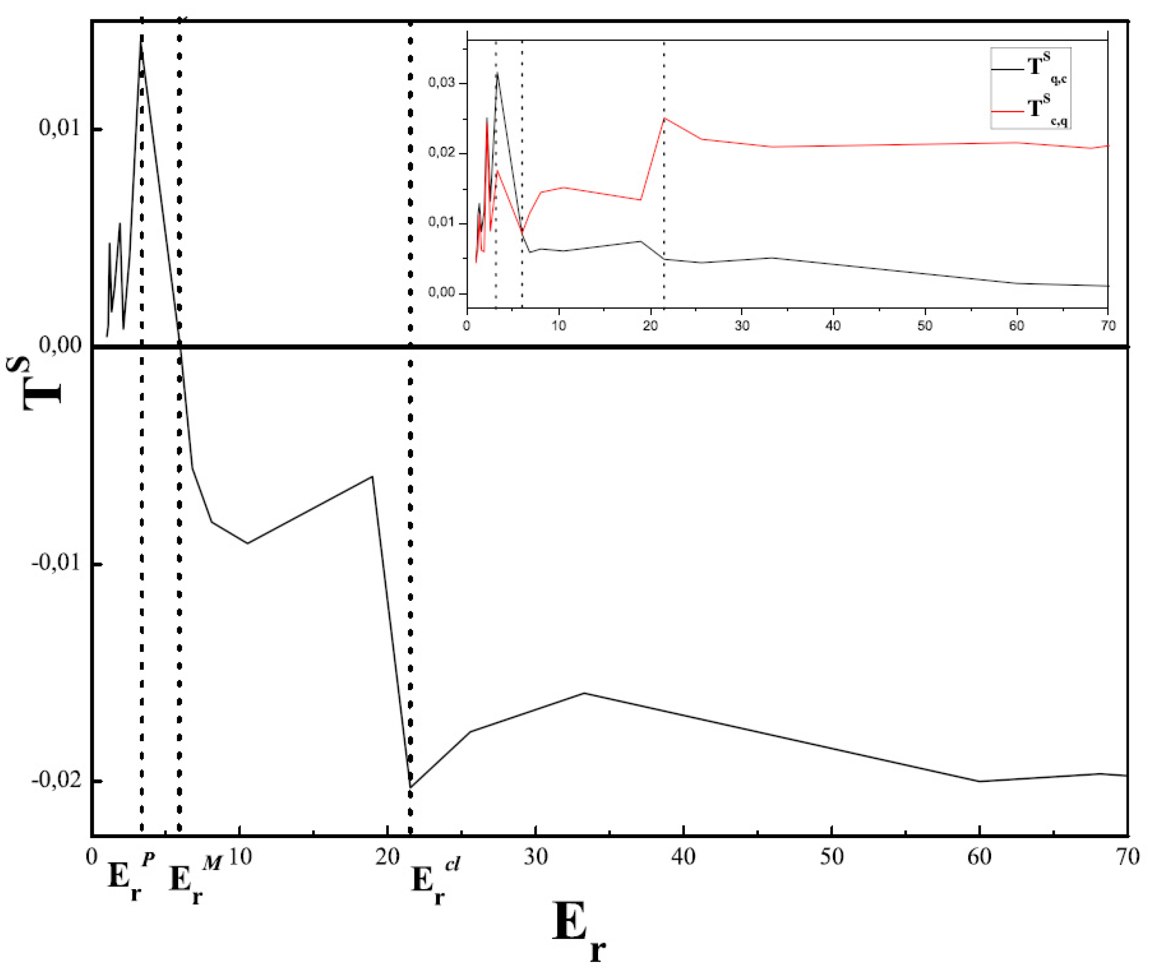
Figure 3 depicts a similar behavior, the variables now being
and
. Any classical-quantal pair of variables will exhibit the same behavior.
As it should be expected, in the quantum zone quantal variables predominate, and vice versa in the classical region. On the other hand, we note that at the symmetric-flow point
, the Statistical Complexity attains a maximum [
29,
30,
31]. We remind the reader the so called Statistical Complexity reflects on the systems’s architecture, being different from zero only if there exist privileged, or more likely states among the accessible ones. It quantifies not only randomness, but the presence of correlational structures as well. The opposite extremes of perfect order and maximal randomness possess no structure to speak of. In between these two special instances, a wide range of possible degrees of physical structure exist, degrees that should be reflected in the features of the underlying probability distribution [
41]. In
Figure 3, the value
does not obtain exactly at
but very near it, with a relative error
. Note that
divides into two sections the transitional region. The information flow in the leftward subregion is from the quantal variables to the classical ones. In the rightward subregions the information flow reverses its sign. In the former sub-zone the quantum-classical mixture characterizes a phase-space with more non-chaotic than chaotic curves while in the other one things turn around [
23].
Figure 1.
a) The directionality index vs. and b) and vs. , for a wide range. We took and . The classical variable A is dominant across most of the range, except for small values, for which Uncertainty Principle becomes important enough that the quantal variable becomes dominant. Note the absolute minimum of at , beginning of the transition region.
Figure 2.
a) The directionality index
vs.
and b)
and
vs.
, for an
range that allows to visualize the three zones of the process, i.e., quantal, transitional, and classic, delimited, respectively, by
, and
. We took
and
as in
Figure 1. Note the absolute minimum of
at
, the local maximum at
, and the absolute maximum close by (
). Symmetric information flow obtains at
(where the Statistical Complexity attains a maximum), well within the transition region. Classical variable
A is the “leading” one from
until this point. For smaller
values,
becomes dominant.
The other interesting points in the
evolution are
and
, at which the transition-zone and the classical one, respectively, begin. At
one detects the presence of an absolute minimum of the directional index
(
Figure 1) that measures the quantum-to-classic subsystems flow. This minimum is to be read as representing maximal influence of the classical variables over the quantal ones. In the vicinity of
(
) we encounter an absolute maximum of
and thus of the quantum-to-classic subsystems flow. There is also a local maximum at
(that becomes absolute if
is evaluated for the pair
-
(
Figure 3)). Thus the transition zone is located within both minimum and maximum values of the classic-to-quantum subsystems flow. The three quantities
,
, and
correctly describe the convergence of our quantal results towards the classical ones, as depicted in
Figure 1 (fluctuations disappear for large enough values of
).
Figure 3.
The directionality index vs. and and vs. (inset). Here we took and . The three stages of the process are visible between and . Note the absolute maximum at . is here slightly off the mark (see text).
Figure 3.
The directionality index vs. and and vs. (inset). Here we took and . The three stages of the process are visible between and . Note the absolute maximum at . is here slightly off the mark (see text).
One can also argue that the present results shed new light on what was called the quantal zone in References [
29,
30,
31]. Strictly speaking, the system of Equation (2) always describes a semiclassical system, for any
. A trivial instance is that of
, in which classical-quantal decoupling takes place. In the vicinity of
the system behaves like a slightly perturbed quantum harmonic oscillator. As
grows, that associated orbits undergo a deformation process, but retain their quasi-periodic nature, as long as
remains within the quantum zone, however the system of Equation (2) does represent a coupled system, entailing that the evolution of the quantal variables depends upon the classical ones. Thus, it is not a trivial fact that we can speak of a quantum zone. That we properly do is now
confirmed in the light of our present results regarding the fact that the quantum variables govern the information flow in this zone.
5. Conclusions
In the present communication we have delved into the classical-quantal frontier problem using as a tool the symbolic transfer entropy for investigating the dynamics generated by a semi-classical Hamiltonian that represents the zero-th mode contribution of an strong external field to the production of charged meson pairs [
6,
23].
The dynamical analysis of the problem performed in Reference [
23] specified the highlights of the road towards classicality of the dynamics of the semi-quantum system in question, via a description in terms of the relative energy
given by Equation (4). As
grows from
(the “pure quantum instance”) to
(
, the classical situation), a significant series of
morphology changes are detected in the solutions of the system of nonlinear coupled equations defined by Equation (2). The concomitant process takes place in three stages: quantal, transitional, and classic, delimited, respectively, by special values of
, namely,
and
. This dynamical description was also reobtained later via statistical treatments in References [
29,
30,
31].
Here we have seen that using the notion of symbolic transfer entropy with its directional index
the problem tackled in these references can be expressed in a different light, namely, as an information flow between classical and quantal variables. We demonstrate that, starting from
leftwards, classical variables lead the process until the effects of the Uncertainty Principle become important enough at
. At this particular value the information flow becomes symmetric and for larger energy values it reverses its sign. We conclude that the Uncertainty Principle is the responsible for this change so that we can associate the flow inversion with the classical-quantal transition. At
the statistical complexity becomes maximal [
29,
30,
31] entailing that symmetry of information flow is tantamount with maximum complexity. We note that
and
are, respectively, points of maximal quantal-classical and maximal classical-quantal information-flows. Additionally, the present results shed new light on what was called the quantal zone, as discussed at the end of the preceding section, as therein the quantum variables do govern the information flow.
Finally, we have shown the efficiency of the new information-quantifier called the symbolic transfer entropy and protagonist of the present considerations, validating its physical significance, which should encourage its application to other problems.


