Maximum Entropy Approaches to Living Neural Networks

Abstract

Understanding how ensembles of neurons collectively interact will be a key step in developing a mechanistic theory of cognitive processes. Recent progress in multineuron recording and analysis techniques has generated tremendous excitement over the physiology of living neural networks. One of the key developments driving this interest is a new class of models based on the principle of maximum entropy. Maximum entropy models have been reported to account for spatial correlation structure in ensembles of neurons recorded from several different types of data. Importantly, these models require only information about the firing rates of individual neurons and their pairwise correlations. If this approach is generally applicable, it would drastically simplify the problem of understanding how neural networks behave. Given the interest in this method, several groups now have worked to extend maximum entropy models to account for temporal correlations. Here, we review how maximum entropy models have been applied to neuronal ensemble data to account for spatial and temporal correlations. We also discuss criticisms of the maximum entropy approach that argue that it is not generally applicable to larger ensembles of neurons. We conclude that future maximum entropy models will need to address three issues: temporal correlations, higher-order correlations, and larger ensemble sizes. Finally, we provide a brief list of topics for future research.

1. Introduction

A great scientific challenge of this century is to describe the principles governing how ensembles of brain cells interact. Neural network models and theories suggest that groups of brain cells, containing tens to thousands of neurons, are collectively able to perform elementary cognitive operations. These operations include pattern recognition, associative memory storage, and coordination of motor actions in complex sequences [1,2,3,4]. Although a thorough understanding of these processes would not completely tell us “how the brain works”, it would bring us closer to developing a theory of mental activity rooted in physical laws.

While we are still far from understanding how networks with a thousand neurons operate, two recent developments have brought us much closer to describing interactions in ensembles containing tens of neurons. First, progress in multineuron physiology has allowed many laboratories to perform long-duration (~1 h) recordings from a hundred or more closely-spaced neurons [5,6,7]. These recordings come from both calcium imaging [8,9] and multielectrode array experiments [10,11]. Second, progress in theory has allowed the field to construct phenomenological models of activity in neuronal ensembles. One of the most popular models in this regard has come from the “maximum entropy” approach, which is the subject of this review [5,12,13]. Also gaining attention, however, have been the efforts made with “Generalized Linear Models (GLMs)” (for a review and application of GLMs, see [14,15]). These models can replicate many of the statistics of neuronal ensembles, and may therefore give us insight as to how tens of neurons interact. Together, these advances have generated tremendous interest in physiology at the neural network level.

What is the maximum entropy approach? Briefly, it provides a way for quantifying the goodness of fit in models that include varying degrees of correlations [16]. To explain this, consider a hierarchy of models, each including progressively more correlations to be fit. A first-order model is one that would seek to fit only the average firing rate of all the neurons recorded in an ensemble. A second-order model is one that would seek to fit both the average firing rates and all pairwise correlations. Similarly, an nth-order model is one that would seek to fit all correlations up to and including those between all n-tuples of neurons in the ensemble. The maximum entropy approach provides a way to uniquely specify each of these models in the hierarchy [17]. It does this by assuming that the best model at a particular level will be the one that fits the correlations found in the data up to that level and that is maximally unconstrained for all higher-order correlations. Relaxing all other constraints can be accomplished by maximizing the entropy of the model, subject to fitting the chosen correlations. By uniquely specifying this hierarchy of models, the maximum entropy approach allows the relative importance of higher-order correlations to be evaluated. For example, this framework permits us to ask whether an accurate description of living neural networks will require fifth-order correlations or not. If so, then describing ensembles of neurons will be a truly difficult task. Alternatively, it could tell us that only second-order correlations are required. Either way, the maximum entropy approach provides us with a way to quantify how accurately we are fitting the system [16].

Why has the maximum entropy approach attracted so much attention? Two groups recently applied maximum entropy methods to neural data with apparent success [5,12]. They sought to describe the distribution of states in ensembles of up to 10 neurons from retinal tissue and dissociated cortical networks. Interestingly, they both reported that, on average, ~90% of the available spatial correlation structure could be accounted for with a second-order model. This result suggested that living neural networks were not as complicated as initially feared. This conclusion has been widely noticed, and many groups have vigorously responded both positively and negatively to the original papers on maximum entropy by [5,12]. At present, this area of research is very active and can be characterized as having healthy and lively discussions. Regardless of how these issues are ultimately resolved, it is likely that maximum entropy approaches to neural network activity will continue to be researched in computational neuroscience for years to come.

Here, we will review all of these developments. This paper is organized into five main parts. First, we will explain the maximum entropy approach as it was originally applied to neural ensemble recordings in 2006 [5,12] so that people unfamiliar with this method will be able to apply it to their data. Second, we will describe the problem that these first models had with temporal dynamics. Third, we will review a very recent attempt to incorporate temporal dynamics. Fourth, we will discuss criticisms and limitations of the maximum entropy approach. Fifth, we will mention topics for future research.

2. Maximum Entropy for Spatial Correlations

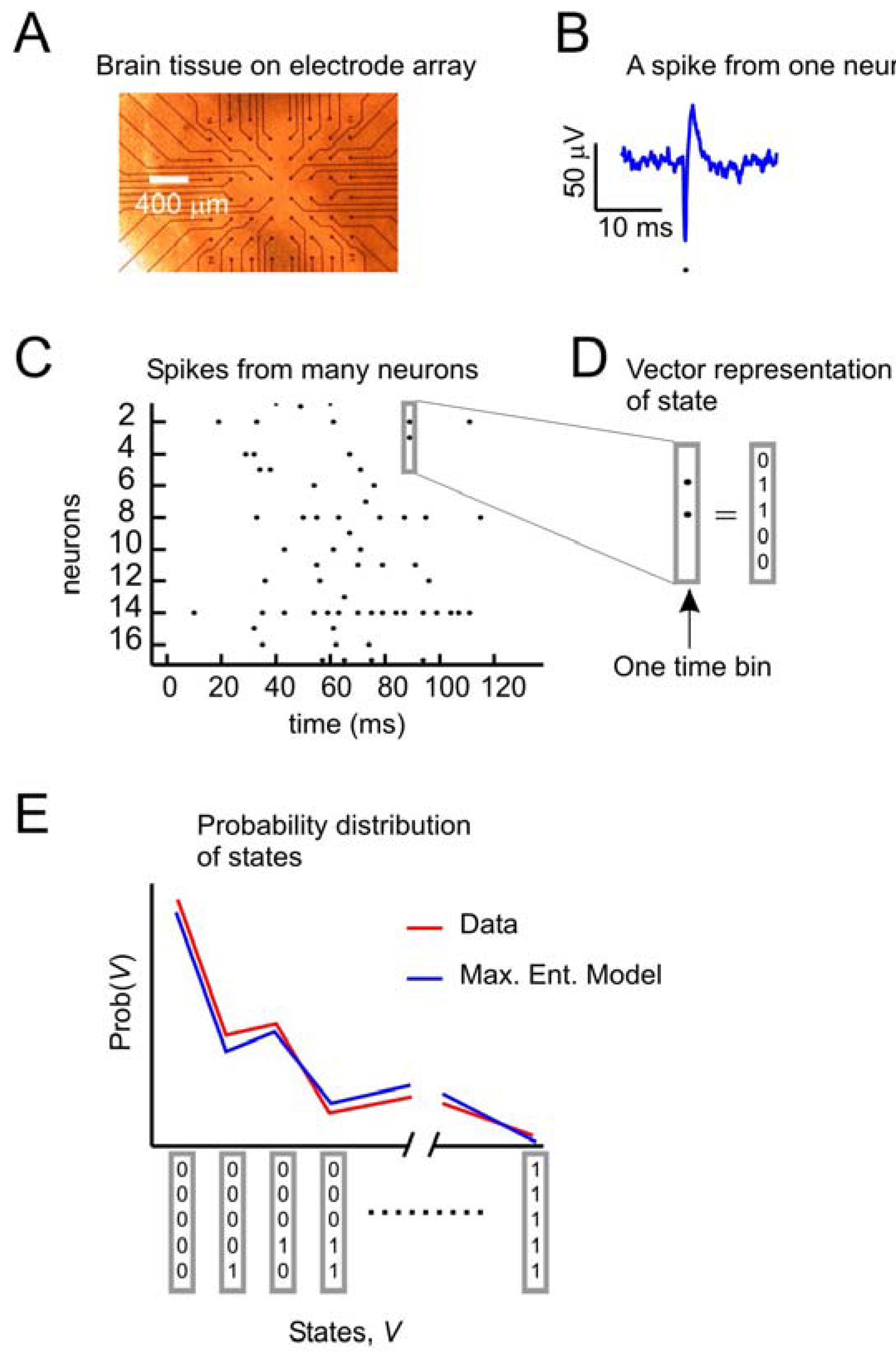
Figure 1 depicts the problem of describing activity states in ensembles of neurons. A small slice of neural tissue (e.g., retina or cortex) is placed on a multielectrode array (Figure 1A), where it can be kept alive for hours if it is bathed in a warm solution containing the appropriate salts, sugars and oxygen. For a full description of the methods used to maintain these tissues and for recording from them with multielectrode arrays, consult [5,12,18]. Under these conditions, the neurons lying over the electrode tips can produce voltage “spikes” when they are active (Figure 1B). Spikes from many neurons over time can be represented as dots in a raster plot (Figure 1C). At any moment, the state of an ensemble of, say, five neurons can be represented by a binary vector (Figure 1D), where 1 s indicates spikes and 0 s indicate the absence of spikes. A first step toward understanding collective activity in these neurons would be to construct a model that could account for the probability distribution of states from the ensemble. The maximum entropy model, as first applied by [5,12] sought to predict the distribution of states with a second-order model, given only information about how often each neuron spiked, and the pairwise correlations of spiking between neurons. Note that in this form of the problem, we are only concerned with the spatial correlations between neurons. As we will see later, there are significant temporal correlations between neurons as well. In what follows, we will recapitulate the approach first used by [5,12] to solve the problem of spatial correlations in neural data. Earlier versions of the maximum entropy approach were first described in [16,17,19,20].

Figure 1. The problem to be solved.

Figure 1. The problem to be solved.

(a) Data from neural tissue are collected with a multielectrode array. Here, a slice of cortex is placed over 60 electrodes (Multichannel Systems). Typically, tens to hundreds of neurons are recorded, but tens of thousands of neurons are in the slice. (b) Activity in individual neurons is detected as very short voltage spikes. The time of minimum voltage is marked by a dot. (c) All spikes from all neurons are plotted over time, where a dot represents the time of a spike. (d) The state of an ensemble of five neurons in one time bin is represented as a vector, where ones indicate spikes and zeros indicate no spikes. Time bins are usually a few milliseconds (4 ms here). (e) The goal of the second-order maximum entropy model is to explain the probability distribution of states found in the data, given only information about the firing rates and pairwise correlations between neurons. Here a schematic probability distribution is shown for data and the model.

Because spiking neural activity is either on (1) or off (0), we can represent the state of each neuron i by a spin, σ_i, that can be either up (+1) or down (–1). There is a rich history of using this binary representation of neural activity in network models [2,21]. To represent temporal activity as a sequence of numbers, the duration of the recording is broken down into time bins. We will discuss the implications of the width of these time bins more in section 5. A typical width is 20 ms, as in [5,12], but other widths have been used also. Thus, a 100 ms recording in which a single spike fired at 23 ms would be represented by the sequence: (–1,+1, –1, –1, –1) if the data were binned at 20 ms. With this representation, the average firing rate of neuron i is given by:

(1)

where T is the total number of time bins in the recording, and the superscript t represents the bin number. The pairwise correlations are given by:

(2)

where the angled brackets indicate temporal averaging.

The state vector, V, represents the state of N spins (out of 2^N possible states) at a particular time bin, and is given by:

(3)

To predict the probability distribution of these states, an analogy with the Ising model from physics [2,22] is made. This is because the equation that specifies the “energy” of the second-order maximum entropy model is the same as that used to specify the energy in the Ising model [12]. Please note that this is only an analogy, as connectivity in the Ising model is strictly between units that are nearest neighbors, whereas connections in neural networks can potentially occur between any neurons. In this model, each spin will have a tendency to point in the same direction as the local magnetic field, h_i, in which it is embedded. In addition, the state of each spin will depend on the interactions it has with its neighbors. When the coupling constant J_ij is positive, spins will have a tendency to align in the same direction; when it is negative, they will have a tendency to be anti-aligned. In this language, the “energy” of an ensemble of N neurons can be given by:

(4)

where summation in the second term is carried out such that i ≠ j. Please note that while this model is mathematically equivalent to the Ising model of a ferromagnet, no one is suggesting that neural firings are primarily influenced by magnetic interactions. Neural interactions are thought to be governed by synapses, which can be described largely by biochemistry and electrostatics [23].

Once energies are assigned to each state in the ensemble, it is possible also to assign a probability to each state. This is done the same way that Boltzmann would have done it, by assuming that the probabilities for the energies are distributed exponentially, in the manner that maximizes entropy [5,12,24,25]:

(5)

where the state vector V_j again represents the jth state of spins and where the denominator is the partition function, summed over all 2^N possible states of the ensemble. Note that this equation will make states with high energy less probable than states with low energy.

Because this distribution gives the probability of each state, the expected values of the individual firing rates 〈σ_i〉_m and pairwise 〈σ_iσ_j〉_m interactions of the maximum entropy model can be extracted by the following equations, where the subscript m denotes model:

(6)

(7)

and where σ_i(V_j) is the activity (either +1 or –1) of σ_i when the ensemble is in state V_j. The expected values from the model are then compared to 〈σ_i〉 and 〈σ_iσ_j〉 found in the data. Although the model parameters are initially selected to match the firing rates and pairwise interactions found in the data, a given set of parameters in general will not produce harmony of every neuron with its local fields and interactions for every state. To improve agreement between 〈σ_i〉_m, 〈σ_iσ_j〉_m and 〈σ_i〉, 〈σ_iσ_j〉, the local magnetic fields h_i and interactions J_ij are adjusted by one of many gradient ascent algorithms [26]. Several groups [12,18] have used iterative scaling [27], as follows:

(8)

(9)

where a constant α < 1 is used to keep the algorithm from becoming unstable. After adjustment, a new set of energies and probabilities is calculated for the states, and this leads to new values of h_i and J_ij. Adjustments can be made iteratively until the local field and interactions are close to their asymptotic values. Because the entropy is convex everywhere in this formulation, there are no local extrema and methods like simulated annealing are not necessary. After iterative scaling, the final values of h_i and J_ij are then re-inserted into equation (4) to calculate the energy of each state, and then this energy is inserted into equation (5) to calculate the probability of observing each state V. This process of adjustment can be time consuming because it is computationally intensive to calculate the averages in equations 6 and 7, which requires summing over 2^N terms. Faster methods have been developed which allow larger numbers of neurons to be analyzed [26,28,29]. These methods exploit ways of approximating the averages in equations 6 and 7.

We now explain how the performance of the model is evaluated. Recall that models of several orders can be used to capture the data. A first-order model accurately represents the firing rates 〈σ_i〉 found in the data, but assumes that all higher-order interactions, like 〈σ_iσ_j〉, are independent and can be given by the product of first-order interactions: 〈σ_iσ_j〉 = 〈σ_i〉·〈σ_i〉. Schneidman and colleagues [12] denoted the probability distribution produced by a first-order model by P₁. A second-order model, as described above, takes into account the firing rates and pairwise interactions, and produces a probability distribution that is denoted by P₂. For an ensemble of N neurons, an accurate N^th-order model would capture all the higher-order interactions found in the data, because its probability distribution, P_N, would be identical with the probability distribution found in the data. The entropy, S, of a distribution, P, is calculated in the standard way:

(10)

Note that the entropy of the first-order model, S₁, is always greater than the entropy of any higher-order models, S₂… S_N, because increased interactions always reduce entropy [12,30]. The multi-information, I_N, is the total amount of entropy produced by an ensemble, and is expressed as the difference between the entropy of the first-order model and entropy of the actual data [12,31]:

(11)

The amount of entropy accounted for by the second-order maximum entropy model is given by:

(12)

The performance of the second-order maximum entropy model is therefore quantified by the fraction of the multi-information that it captures, denoted by the ratio r:

(13)

This fraction can range between 0 and 1, with 1 giving perfect performance. When the values of h_i and J_ij are computed exactly, the ratio can also be expressed as [5,30]:

(14)

where D₁ is the Kullback-Leibler divergence between P₁ and P_N, given by:

(15)

and D₂ is the Kullback-Leibler divergence between P₂ and P_N:

(16)

Shlens and colleagues used a ratio derived from the Kullback Leibler divergence [5], while Schneidman and colleagues used a ratio of multi-information [12]. When both of these groups applied the second-order model to their data, they found that it produced ratios near 0.90 on average, meaning that the model could account for about 90% of the spatial correlation structure [5,12]. While this suggests that the model predicted the probabilities of most states correctly, it is worth noting that even with ratios near 0.90, these models still failed to accurately predict the probability of some states by several orders of magnitude. An intuitive way to think about this ratio r in equation (13) is that it measures how much better a second-order maximum entropy model would do than a first-order model. From this perspective, some errors are unsurprising.

Another particularly important potential source of error arises from estimating the entropy of a distribution of states produced by an ensemble of spike trains. Generally, if the firing rates of the neurons are relatively low and the recording duration is short, there may not be enough data to adequately sample the distribution of all possible states, making estimates of the entropy inaccurate. This problem becomes exponentially worse as the number of neurons in the ensemble increases [32,33,34].

Aware of this issue, Shlens and colleagues noted that each of all the binary states in their recordings occurred 100–1,000 times [5], indicating minimal errors. Schneidman and colleagues noted that all of their recordings were on the order of one hour long, which they argued made undersampling unlikely for their firing rates [12]. There is a large literature on methods of entropy estimation [32,34,35,36], and this area is being actively researched. The main point here is that entropy estimation errors may lead to inaccuracies in the maximum entropy model, even if values of r appear to be high. Long recordings are necessary to minimize these errors.

3. The Issue of Temporal Correlations

After these relatively high ratios were reported, it appeared that the maximum entropy model could account for spatial correlations, at least in relatively small ensembles of neurons (N = 4 to 10). But brains are faced with the task of responding to patterns in space and time. It was therefore of interest to see whether temporal correlations played a substantial role in the activity generated by samples of brain tissue. If they did, future models of ensemble activity would need to account for temporal as well as spatial structure.

Tang and colleagues [18] looked at the issue of temporal correlations in a very elementary way. If correlations across time were relatively unimportant, they reasoned, activity states in an ensemble of neurons would occur in random order, with no particular preference for one state to be followed by another.

To test this, they compared the distribution of sequence lengths in actual neural ensembles with those generated by randomly selecting states from the model. Here, a “sequence” of length L was defined as L time bins in which at least one neuron was active in every time bin (Figure 2). Also, a sequence had to be bracketed at the beginning and at the end by time bins with no activity, as shown in Figure 2B.

Interestingly, they found that most sequence lengths from the data were significantly longer than those randomly drawn from the maximum entropy model (Figure 2C). This indicated that temporal correlations were important, and challenged future maximum entropy models to account for them. While this was an important step forward, it was still unclear whether temporal correlations played a major or a minor role in governing activity in neural ensembles.

Figure 2. Temporal correlations are important. (a) Activity from many neurons plotted over time. Boxes highlight an ensemble of four neurons over six time bins. (b) Within the boxes, there was activity for four consecutive time bins, bracketed by no activity at the beginning and the end. This is a sequence of length L = 4 (see text). (c) Sequence length distributions from actual data were significantly longer than those produced by random concatenations of states from the model. This suggests that temporal correlations play an important part in determining activity in neuronal ensembles.

Figure 2. Temporal correlations are important. (a) Activity from many neurons plotted over time. Boxes highlight an ensemble of four neurons over six time bins. (b) Within the boxes, there was activity for four consecutive time bins, bracketed by no activity at the beginning and the end. This is a sequence of length L = 4 (see text). (c) Sequence length distributions from actual data were significantly longer than those produced by random concatenations of states from the model. This suggests that temporal correlations play an important part in determining activity in neuronal ensembles.

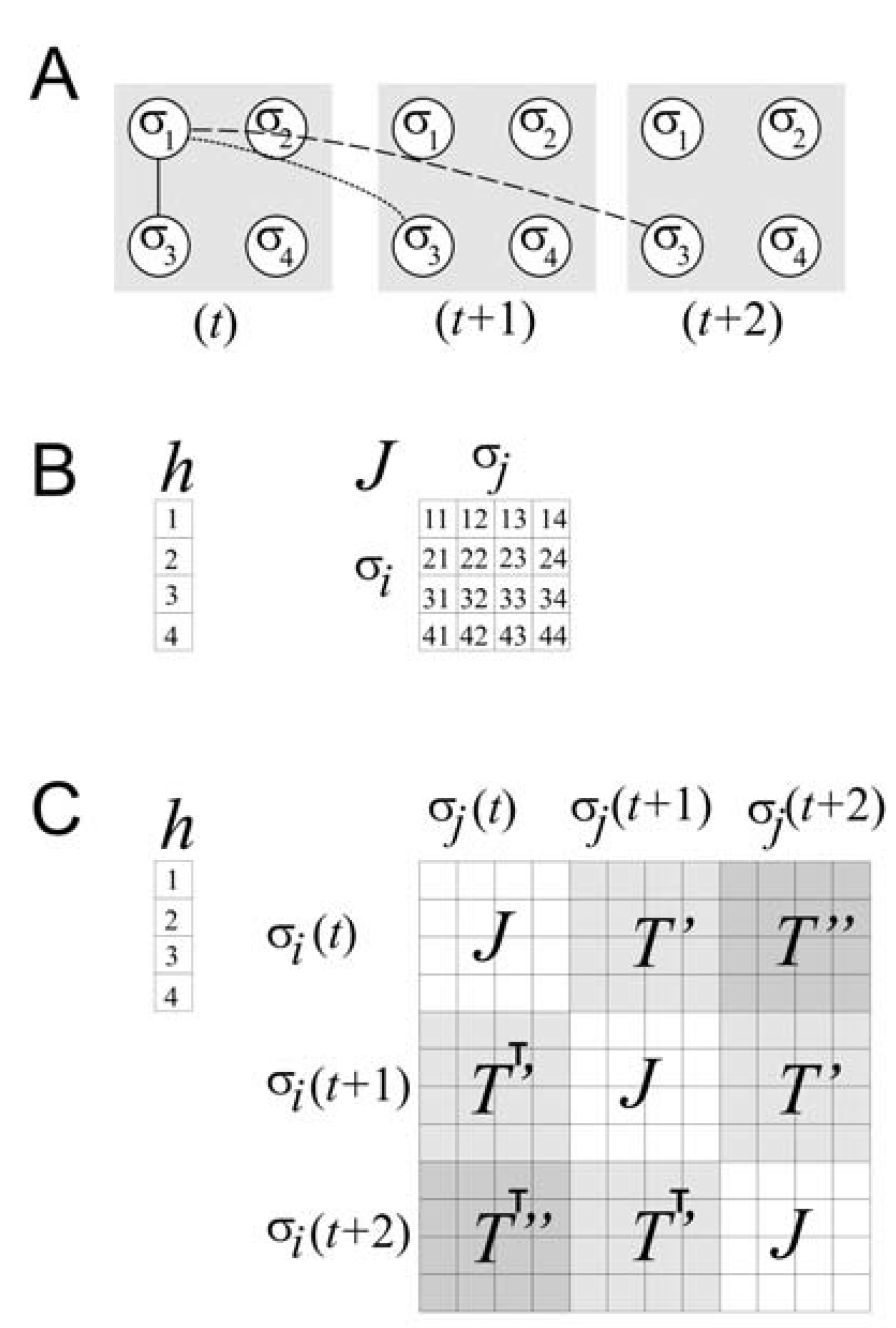
4. Incorporating Temporal Correlations

Soon after it became clear that temporal correlations were important, Marre and coworkers modified the existing maximum entropy model to account for them [37]. Here we will overview how they did this, and how this ultimately led to an estimate of the relative importance of temporal correlations, something that we consider to be a very significant advancement. Marre and colleagues realized that if temporal correlations were to be included, the new expression for the energy had to have the form:

(17)

where now the state vector V represents a particular state of N spins at times t, t + 1, and t + 2. The terms T’ and T’’ are temporal coupling constants, relating spins to each other across one and two time steps, respectively. For simplicity, here we will consider only temporal correlations two time steps into the future. We could account for more time steps simply by adding more T terms, but this dramatically increases the dimensionality of the problem, as we will discuss more later. Although all of these additional terms might seem to complicate the optimization process, it is still possible to combine each matrix of temporal couplings (T’ and T’’) with the original matrix of spatial couplings (J) so that they form one large composite matrix. This is shown in Figure 3. In this form the adjustment of model parameters can take place just as before, using iterative scaling, for example, on the terms in h, J, T’ and T’’.

Figure 3. Accounting for temporal correlations.

Figure 3. Accounting for temporal correlations.

(a) Schematic of a four spin system at three different time steps (t, t + 1, and t + 2). For simplicity, only the correlations between σ₁ and σ₃ are shown over space and time. The solid line represents spatial correlation; the dotted line represents temporal correlation one time step into the future; the dashed line represents temporal correlation two time steps into the future. (b) Matrices required for the model only of spatial correlations for the four spin system. The local magnetic field is represented by h, and the spatial coupling constants by J. (c) Composite matrix required for the model of spatial and temporal correlations up to two time steps for the four spin system. The local magnetic field h is as before, but the matrix of coupling constants is considerably expanded. The matrix of spatial coupling constants J occurs whenever interactions among spins at the same time step occur. The matrices of temporal coupling constants, T’ and T’’, occur whenever there are interactions among spins at temporal delays of one and two time steps, respectively. Note that transposed matrices are used below the diagonal, indicating that delayed correlations are treated here as if they are symmetric in time, following [37].

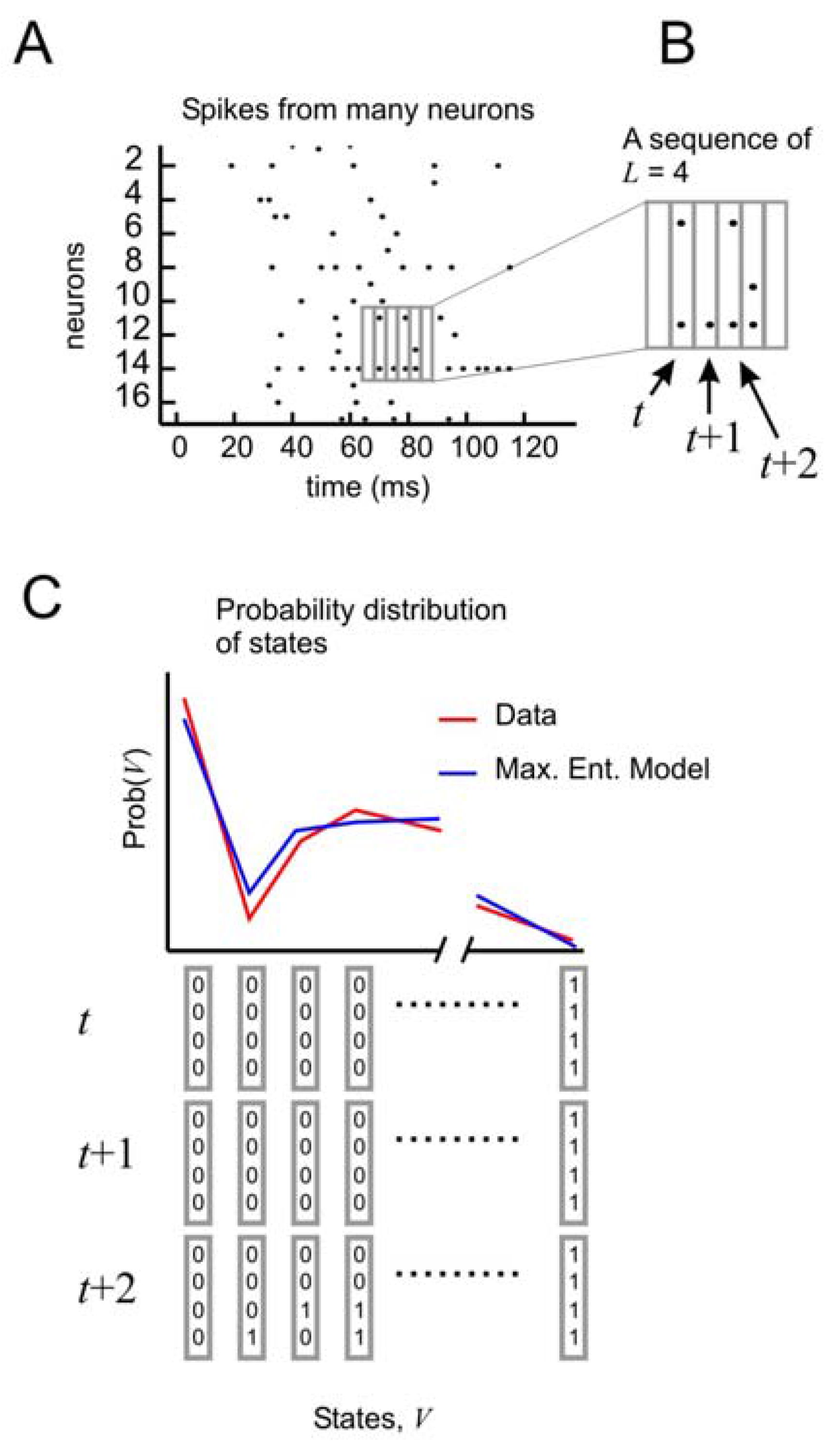
To test the performance of this model, it is necessary to consider the distribution of states of N spins at times t, t + 1, and t + 2 (Figure 4A, B). In this formulation, the state vector has 3N elements, and can take on 2^3N different configurations. As before, the probability distribution of these states from the data is compared to the distribution produced by the model (Figure 4C). But now it is possible to tease out the relative importance of spatial and temporal correlations. This can be done by creating three different types of models: one that accounts for spatial correlations only, one that accounts for spatial correlations and temporal correlations only one time step ahead, and one that accounts for spatial correlations and temporal correlations two time steps ahead.

Figure 4. Distribution of states for a model with temporal correlations (a) An ensemble of four neurons is selected from the raster plot. (b) Here, activity over a span of three time bins (t, t + 1, and t + 2) is considered one state. (c) The distribution of states is plotted for the model and for the data.

Figure 4. Distribution of states for a model with temporal correlations (a) An ensemble of four neurons is selected from the raster plot. (b) Here, activity over a span of three time bins (t, t + 1, and t + 2) is considered one state. (c) The distribution of states is plotted for the model and for the data.

All of these models can be made to produce a distribution of states for N neurons over three time steps. For the model that only has spatial correlations, states are randomly drawn from the distribution and concatenated into sequences of length 3. For the model with temporal correlations of one time step, the first state is randomly drawn and subsequent states are then drawn from the subset of states in the distribution whose first time step matches the last time step of the previous state. In this way, the configuration of activity found in N neurons always changes in time in a manner that agrees with the temporal correlations found in the distribution produced by the model. The model with temporal correlations of two time steps already has a distribution of 2^3N states and does not need to be concatenated to produce states of three time steps. Once temporal distributions for all three models are obtained, they can be compared as before by using a ratio of multi-information. The results of this comparison are shown in Figure 5.

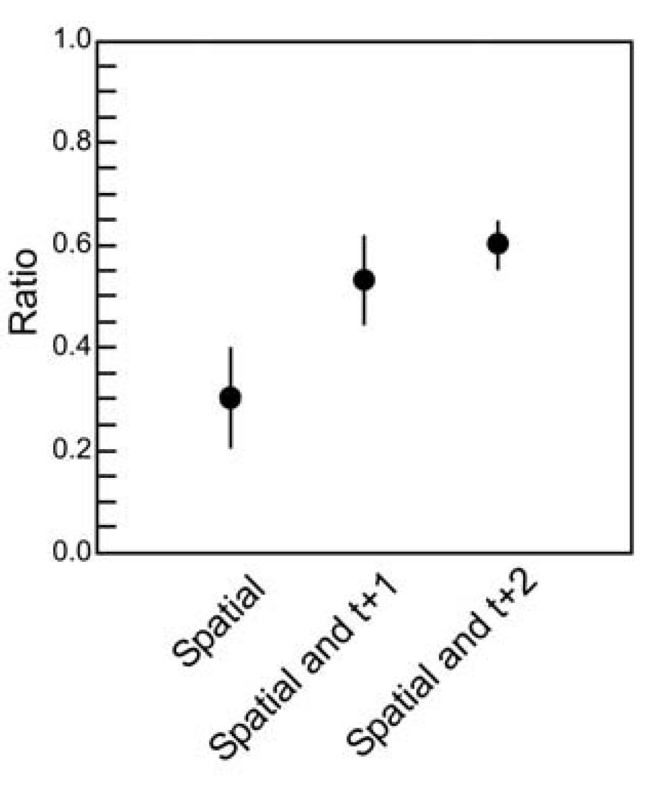
Figure 5. Quantifying temporal correlations.

Figure 5. Quantifying temporal correlations.

The ratio of multi-information (see text) is plotted for the three maximum entropy models: One that accounts for spatial correlations only; one that accounts for spatial and temporal correlations of one time step; one that accounts for spatial and temporal correlations of two time steps. Ratios were obtained for ten ensembles of four neurons (N = 4), each drawn from a slice of cultured cortical tissue prepared by the Beggs lab. Error bars indicate standard deviations. Here, all three models were evaluated on the basis of how well they accounted for the distribution of states containing three time steps, where there were 2^3N = 4096 possible states. Note that this number is far more than the number of states in the spatial task, where 2^N = 16. Because the dimensionality has increased dramatically, it is perhaps not surprising that the ratios are below 0.65, the value obtained when spatial models were applied to spatial correlations only between spiking neurons in cortical tissue for N = 4 [18]. Adding more temporal correlations to the model clearly improves its performance, but also reveals a fraction of temporal correlations that are not captured by the model. These preliminary results should be interpreted with caution, however, as they are obtained from a relatively small ensemble size. Calculations for larger ensemble sizes are challenging because of the dramatic increase in dimensionality.

Although this is only a small sample from which to draw conclusions, three features of this result are worth highlighting. First, note that the ratios here are below the ~0.65 ratio values obtained when the spatial model was applied to spatial correlations alone between (N = 4) spiking neurons in cortical tissue [18]. In interpreting this result, we must remember that the dimensionality of the temporal problem (2^3N = 4,096) is substantially greater than the dimensionality of the spatial problem (2^N = 16). If temporal correlations play any role, it would therefore be reasonable to expect a somewhat lower ratio when only one or no time steps are included in the model. Second, note that including two time steps of temporal correlations nearly doubles the ratio obtained by the spatial model. This quantifies how important temporal correlations are: they account for roughly half of the correlation structure captured by the model. Third, note that even when two time steps are included in the model, a portion of correlations in the data are still unaccounted for. For example, if we were to fit the three points in the plot with an exponential curve, it would asymptote somewhere near 0.75, suggesting that about 25% of the spatio-temporal correlation structure would not be captured by the model, even if we were to include an infinite number of temporal terms in our correlation matrix. Conclusions here are preliminary, though, as this example is taken from a small sample of neurons prepared by our lab. For example, it is presently unclear whether an exponential function, rather than a linear one, should be used here. We are in the process of analyzing larger samples of neurons to clarify this issue. Despite the fact that the temporally extended maximum entropy model is not able to account for some fraction of correlations, the model still may be useful in giving us insight as to how correlations are apportioned in ensembles of living neural networks. This issue was not previously appreciated, and represents a gap that must be filled by future generations of models [18,37,38].

In some ways, the fact that all of the spatio-temporal correlations are not captured is not surprising. The maximum entropy models used here are all related to the Ising model. In this formulation, correlations between neurons are assumed to be symmetric in time. But abundant evidence indicates that neural interactions over time are directional and therefore asymmetric [15,39,40]. In addition, the Ising model is strictly appropriate only for problems in equilibrium statistical mechanics; it can tell us how spins in a magnetic material will align at a given temperature only after the material has been allowed to settle, without further perturbations. A local neural network is probably not an equilibrium system, however, as neurons are constantly receiving inputs from other neurons outside the recording area. For neural networks, non-equilibrium statistical mechanics may be more appropriate. Unfortunately, this branch of physics is still undergoing fundamental developments, and the question of how to theoretically treat non-equilibrium systems is still very much open [41,42].

5. Limitations and Criticisms

A serious issue of concern is how well the model scales with the ensemble size, N. Ideally, one would like to apply the model to ensembles of N ≥ 100 neurons, as many current experiments are based on simultaneous recordings from populations of this size [7,10,11,43]. Several issues may make it difficult to extend maximum entropy models to larger ensembles, though.

The first challenge is computational and is rooted in the problem that 2^N states are needed for the spatial model and 2^3N states are needed for the temporal model with only three time steps. Here, two types of solutions are relevant: exact and approximate. When N ≥ 30, it becomes computationally unmanageable to solve these models exactly. If we are interested in approximations, however, it is possible to work with much larger values of N. Several groups have worked on ways to rapidly approximate the model for relatively large ensembles [44,45]. These approximations, however, were performed only for the second-order model. In both the exact and the approximate cases, solving the model for large numbers of neurons is computationally challenging. It seems likely that we will be able to record from more neurons than we can analyze for many years to come.

Another issue related to large N is that exponentially more data are needed to accurately estimate entropy, as mentioned previously in section 2. Recall that the number of possible states in an ensemble of N neurons is given by 2^TN for the spatio-temporal correlation problem, where T is the number of time steps to be included in the model. For an ensemble of ten neurons to be modeled over three time bins, it would take ~ 3.4 years of recording to ensure that each bin in the distribution of states was populated 100 times, even if the ensemble marched through each binary state at the rate of one per millisecond. This is of course a very conservative estimate, as it is unreasonable to assume that each state would be visited in such a manner. The criterion of 100 instances per bin was used by Shlens and colleagues for minimal entropy estimation bias [5]. Such long recordings are obviously unattainable, so entropy estimation errors are inevitable.

Roudi and colleagues [33] have brought up a different set of concerns related to N. They argue that second-order maximum entropy models that seem to work for relatively small ensembles of neurons are not informative for large ensembles of neurons. They showed that there is a critical size, N_c, that is given by:

(18)

where ν is the average firing rate of the neurons in the ensemble and δt is the size of the time bin. For many data sets, ν ·δt ≈ 0.03, giving N_c ≈ 33. When the number of neurons in the ensemble is below this critical size (N < N_c), results from the model are not predictive of the behavior of larger ensembles. But when the size of the ensemble is above this critical size (N > N_c), the model may accurately represent the behavior of larger networks. Thus, Roudi et al. [33] would argue that the results reported by [12] and [18] are not really surprising, as these ensemble sizes are below the critical size, where a good fit is to be expected. In the case of Shelns et al. [5], however, this is not true, as their neurons had very high firing rates and thus had a relatively small critical ensemble size. Indeed, when Shlens and colleagues examined whether or not the model fit for ensembles of up to 100 neurons in the retina, they found that it fit quite well [10]. All of this is consistent with the arguments presented in [33]. These results in the retina are promising, but the circuitry there is specialized and it remains to be seen whether similar results can be obtained in cortical tissue. One way to overcome the critical size restriction would be to increase the bin width, δt, which could bring N_c down to a reasonable size, particularly if the neurons are firing at a high rate. Roudi and colleagues point out that this could create other problems, though, as temporal correlations will be lost when large bin widths are used. We should note that these arguments about a critical size are based on the assumption that the model under consideration is second-order only [33]. These arguments may not apply if higher-order models are used.

But models with higher-order correlations pose challenges of their own. One of the main reasons the maximum entropy approach to neural networks [5,12] generated interest was because it suggested that neuronal ensembles could be understood with relatively simple models. If almost all the spatial correlation structure could be reproduced without knowledge of higher-order correlations, it seemed that there would be no need to include coupling constants for interactions involving three or more neurons. While this result indeed seems to hold true in papers where the maximum entropy model was applied to retinal neurons [5,10,12], it should be noted that work using cortical tissue indicated that somewhat less of the spatial correlation structure could be accounted for by a second-order model [18,38]. This result raised the possibility that higher-order correlations are more abundant in the cortex than in the retina, a conjecture that awaits more rigorous testing. A third-order coupling constant could account for situations where two input neurons would drive a third neuron over threshold only when both inputs were simultaneously active. If the cortex is to compute, it seems obvious that this type of synergistic operation must be present. But including third-order correlations will again greatly expand the amount of computational power needed to develop an accurate model. Future maximum entropy models of large ensembles of cortical neurons will necessarily be computationally challenging.

6. Future Directions

Here we present a brief list of some topics for future research in the area of maximum entropy models. Several of these problems are already being actively researched:

How does the performance of maximum entropy models compare with that of generalized linear models (GLMs) [14]? Are there circumstances in which one model is clearly better than the other?

When extending the maximum entropy model in time, is it possible to have temporally asymmetric couplings in the matrices T’ and T’’? If so, does this significantly improve performance over the case where the couplings are symmetric?

How do maximum entropy models constructed with data from spontaneous activity differ from models constructed with data where responses were conditioned on a stimulus?

Can maximum entropy models generally be used to make inferences about network connectivity, as was done by Yu and colleagues [38]? How do such inferred networks differ from those obtained by measures of effective connectivity [46,47]?

Do the highly correlated states identified by the maximum entropy model really constitute a type of error-correcting code, as was originally claimed by Schneidman and colleagues [12]?

Maximum entropy models take as inputs average values of firing rates and pairwise correlations. To what extent does averaging obscure more subtle, higher-order interactions?

Can ways be found to construct accurate maximum entropy models for large ensembles of neurons from recordings only one or two hours long? Can approximations or inferences greatly ease this sampling problem [28]?

7. Conclusions

Maximum entropy models of neuronal ensembles have been reported to perform well in capturing spatial correlation structure for ensembles of about 10 neurons. It remains to be seen whether these models can be successfully extended to larger ensemble sizes in cortical tissue. In addition, temporal correlations may make up about half of the available correlations in neuronal ensembles. The original maximum entropy model for spatial correlations has been augmented to include temporal correlations, but even when extended, it fails to capture a substantial portion of spatio-temporal correlations. This weakness may be because these models are rooted in equilibrium statistical mechanics; perhaps the brain should be viewed more appropriately as a non-equilibrium system. Future versions of maximum entropy models will be challenged to account for three things: (1) temporal activity, (2) activity in large ensembles of neurons (N ≥ 30) and (3) higher-order correlations.

As maximum entropy models become more complex to better match these aspects of the data, they inevitably will become less similar to the Ising model from which they are descended. In the limit, this approach could develop into a very complicated data fitting exercise. Such an exercise would not necessarily be bad, but the original aim of applying statistical mechanics to the brain will have been lost. The hope was that we may have only needed to know a few details and one principle: construct the model so as to maximize entropy. The reality at this point is still unclear, but it appears that we will need to know many more details. Because of this, we might need to know more than one principle as well. What these principles are, or even if they exist at all, is still an open question.

This problem is not limited to neural networks, but is common to complex systems in general. It is not yet clear whether a conceptual revolution, like those brought on by Copernicus in astronomy, Heisenberg and Schrodinger in quantum mechanics, or Einstein in relativity, is in the future of neuroscience. But it is encouraging to note that the painstakingly adjusted epicycles of Tycho Brahe eventually gave way to the more principled descriptions of Kepler, which finally set the stage for Newton’s great synthesis [48]. We can only hope that more detailed descriptions of living neural networks will provide pave the way for a similar transformation in our conception of the brain.