Uncertainty Analysis of Decomposition Level Choice in Wavelet Threshold De-Noising

Abstract

In this paper, the complexities of various noises, which are quantified by wavelet energy entropy (WEE) and differential coefficient of WEE (D(WEE)), were first analyzed and their uncertainties then estimated and described using confidence intervals. Then, quantitative criterion for judging the WEE and D(WEE) difference between noisy series and noise was put forward, based on which the decomposition level (DL) choice method in wavelet threshold de-noising proposed in 2010 by Sang et al. was improved. Finally, analytical results from examples verified the performance of the improved method, and also demonstrated its much wider applicability; moreover, the DL chosen using it is more reliable because of the fact that uncertainty is taken into consideration.

1. Introduction

This paper considers the problem of choosing decomposition level in wavelet threshold de-noising (WTD). De-noising is a substantial issue in time series analysis because noise contaminates the real signals in observed series data [1,2,3,4,5]. Among the de-noising methods presently used, the WTD one is comparatively superior and is especially applicable for time series with non-stationary and multi-temporal scale characteristics, because it can elucidate the localized characteristics of time series both in the temporal and frequency domains [6,7,8]. The theoretical details of WTD have been described in a large number of contributions such as in [9,10,11,12,13], so they are not repeated here. Although being theoretically effective and widely applied in various engineering activities and applied research fields, in practice the WTD method is influenced by several key issues such as the choice of wavelet [6,14,15,16], threshold estimation [10,11,13,17,18] and the choice of thresholding rules [9,19,20,21], and many studies have been conducted in various fields to solve them.

Besides the three mentioned above the choice of decomposition level (DL) is another key issue, but it is little studied presently, and no effective approaches can be followed to solve it. The white noise testing commonly used for DL choice in WTD cannot identify the real signals in observed series data and thus cannot meet the practical needs well [22]. The authors proposed in [23] a method of choosing DLs to improve wavelet threshold de-noising, whose basic idea is first to compare the difference of energy distributions between noisy series and noise, which are described by wavelet energy entropy (WEE), and then to choose the appropriate DL. Analyses of various examples verified the effectiveness of the proposed method, but in the analytic process by using it, the strictly quantitative criterion for comparing the difference of WEE was not given, therefore the chosen DL results based on the “extreme” would have inherent uncertainty.

In this study, the objective is to propose the criterion for quantifying the WEE difference between noisy series and noise by taking uncertainty into consideration, and to thus improve the DL choice method proposed in [23]. To achieve this purpose, in Section 2, the variations of WEE of various noises are analyzed and their uncertainties are described by using confidence intervals; then the DL choice method given in [23] is amended and improved. In Section 3, we verify the performance of the improved method by analysis of both synthetic and observed series, and further discuss its applicability. Finally, this study is summarized and our conclusions presented in the last section.

2. Uncertainty Analysis in Choosing Decomposition Level

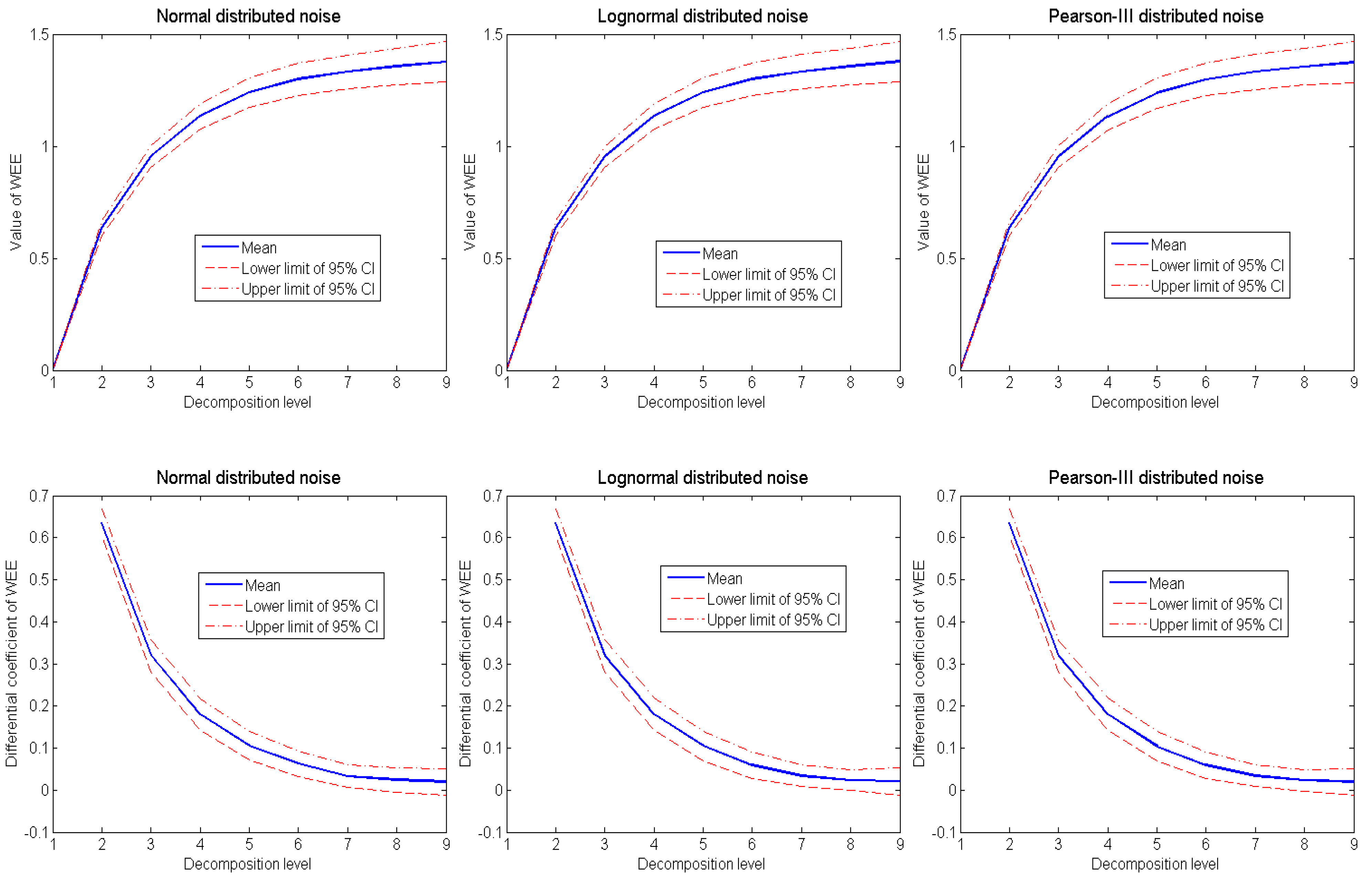
2.1. Complexity of Noises

We first estimate the uncertainty of noises’ complexity by doing the same Monte-Carlo (MC) test as stated in [23]. In the process of noise analysis using the dyadic discrete wavelet transform (DWT), considering that results obtained by different wavelets are the same, the “coif5” wavelet is used as example and the theoretical maximum M of DL is calculated as [24]:

$$M=[{\log }_2(n_{f(t)})]$$

(1)

where [∙] means the integer part of the real value in square brackets and n_f(t) is the length n of series f(t). For the generated noises with the same length of 1,000, the calculated M is 9. Detailed wavelet coefficients of noises are analyzed here to provide useful suggestions for choosing DLs.

To continue, we quantify and describe the complexity of noises by using the wavelet energy entropy (WEE). Specifically, we use each value M_i of the DLs from 1 to 9 and apply dyadic DWT to noises, then reconstruct the sub-signal under each level. Finally, we calculate the value of WEE using Equation (2):

$$\begin{array}{l}WEE(i)=-{\displaystyle \sum _{j=1}^{M_i}{P}_j\ln P_j}with\\ P_j=E_j/{\displaystyle \sum _{j=1}^{M_i}{E}_j={\displaystyle \sum _{t=1}^n{(f_j(t))}^2}/{\displaystyle \sum _{j=1}^{M_i}({\displaystyle \sum _{t=1}^n{(f_j(t))}^2})}}{M}_i=1,\cdots ,M\end{array}$$

(2)

in which n is series’ length, and t is the data number. f_j(t) is the sub-signal under DL j. The WEE is defined according to the concept of Shannon entropy [25], which quantifies series’ complexity. Then, we also calculate the differential coefficients of WEE using Equation (3):

$$D(j)=\frac{d(WEE)}{d(DL)}=\frac{WEE(j)-WEE(j-1)}{j-(j-1)}=WEE(j)-WEE(j-1)$$

(3)

where D(j) is the differential coefficient of WEE under the DL j, and d(∙) means the derivation calculus.

Finally, we calculate the statistical characters of the MC testing results of noises’ WEE and differential coefficient of WEE, D(WEE) for short, including mean ($\overline{X}$) and standard deviation (σ), based on which we estimate their 95% confidence intervals under different DL scenarios.

Figure 1. Values of wavelet energy entropy (WEE) and differential coefficient of WEE (D(WEE)) of various noises, and the corresponding 95% confidence interval (CI) obtained by using different decomposition levels (DLs).

Figure 1. Values of wavelet energy entropy (WEE) and differential coefficient of WEE (D(WEE)) of various noises, and the corresponding 95% confidence interval (CI) obtained by using different decomposition levels (DLs).

The analytical results of various noises’ WEE are depicted in Figure 1, which indicates that the value of WEE increases with DL, so the degree of complexity of noise can be revealed and presented guardedly, and it reaches the maximum when using DL9. However, the value of D(WEE) decreases with DL, and its value under DL9 is close to 0. Furthermore, the 95% confidence intervals (CIs) of both WEE and D(WEE) expand with the increasing DL, and their upper and lower limits are symmetrical about the mean value under each DL, which indicates that they follow the normal probability distribution. Besides, it can be found that for those noises which follow normal, lognormal and Pearson-III distributions, the variations of their complexities, including both the WEE value and the corresponding 95% confidence intervals, are very close to each other. This conclusion is favorable to both the DL choice and uncertainty estimation, as discussed in the following sub-section.

2.2. The Improved Method of Choosing DL

According to the analytical results of noises’ complexity, we amend and improve the DL choice method proposed in [23]. To make this improved method more clear and understandable, we completely describe it in Figure 2 and also explain its analytic steps as follows:

(1)

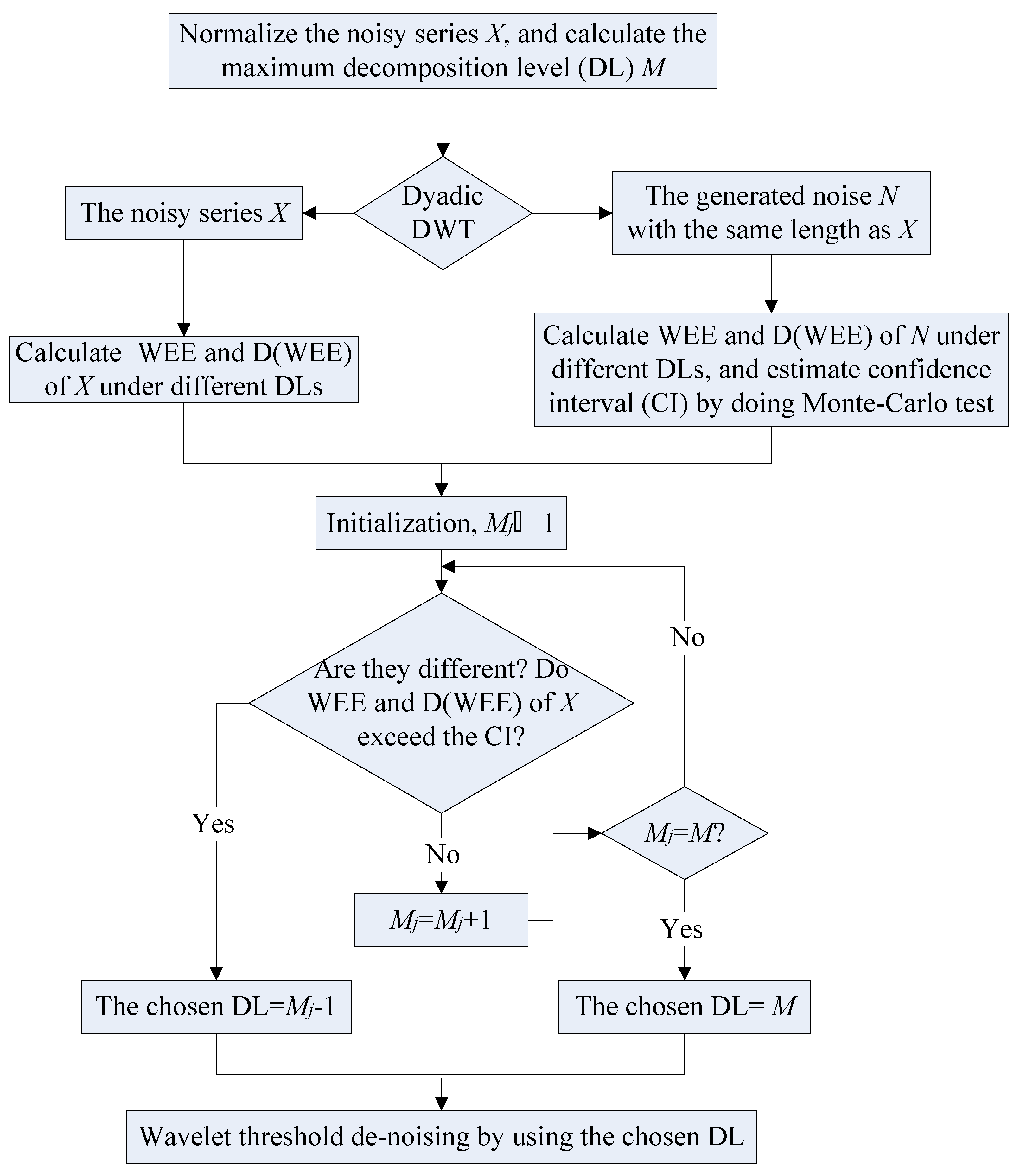
For the noisy series X analyzed, we first calculate the theoretical maximum M of DL by Equation (1), and normalize it by Equation (4):

$$X=\frac{(X-\overline{X})}{\sigma (X)}$$

(4)

in which $\overline{X}$ and σ(X) are the mean and standard deviation of X, respectively.

(2)

Then, we apply dyadic DWT to X by using each value of the DLs from 1 to M, and calculate the values of WEE and D(WEE) by Equation (2) and Equation (3) respectively, based on which we obtain the curves of WEE and D(WEE) of X.

(3)

According to the practical situations and experiences, we choose an appropriate probability distribution to generate “normalized” noise with the same length as that of X. Then we determine the curves of WEE and D(WEE) of noise by doing Monte-Carlo test, and also estimate the confidence intervals of them with a proper significance level (e.g., 5%).

(4)

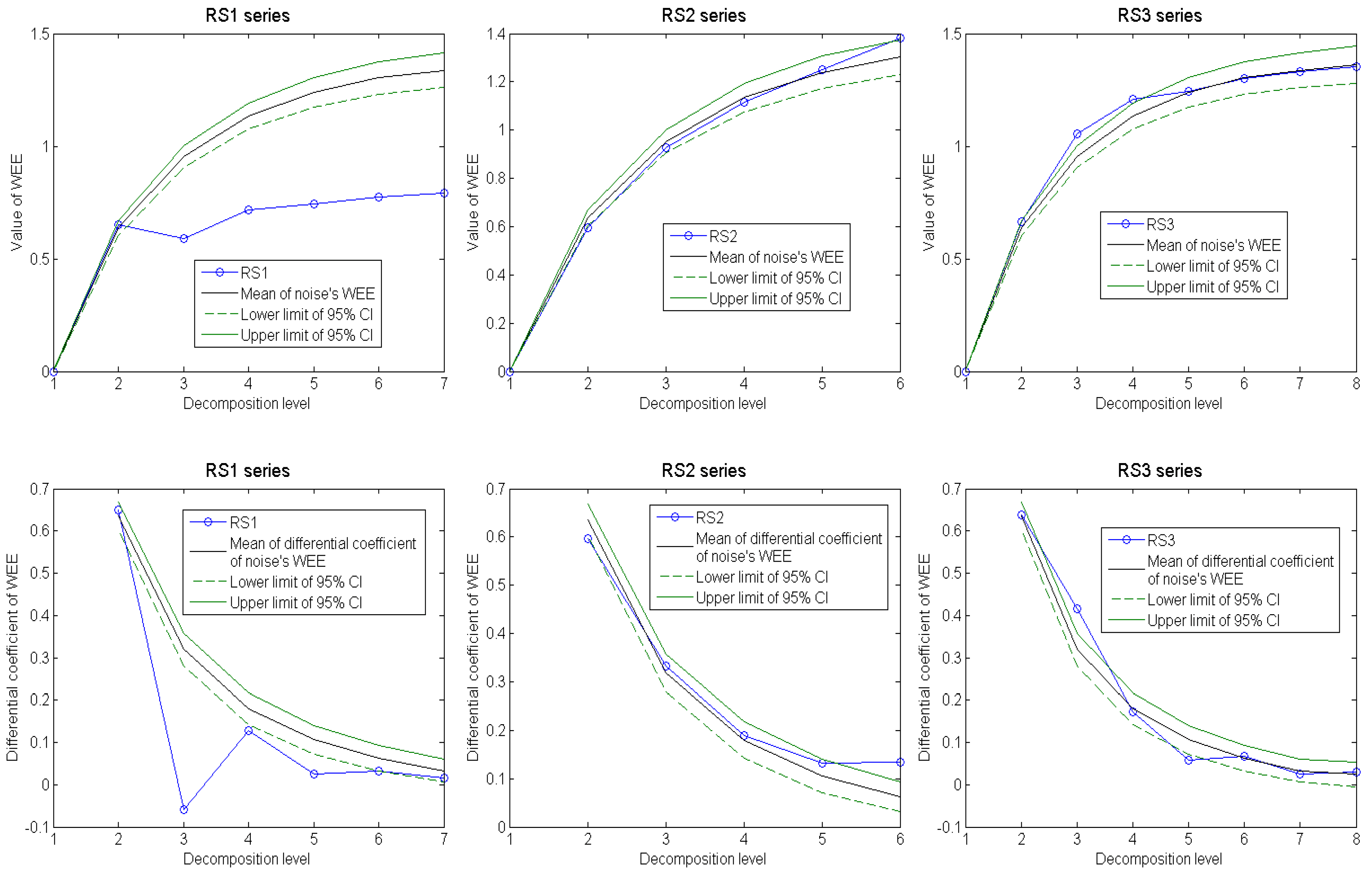
Finally, we compare the value of WEE, especially D(WEE), of the noisy series X with those of noise with the increasing of DLs. Once the values of D(WEE) and WEE of X are obviously different from those of noise and exceed the confidence interval under certain DL^*, the best DL can be chosen as DL^* less 1. Besides, if the values of WEE and D(WEE) of X are close to those of noise under all DLs, the noisy series X can be regarded as a random series.

As explained in [23], the improved DL choice method in WTD is based on the complexity difference between noisy series and noise, thus it has a dependable physical basis. Besides, it is easy to perform because in practice the need for generating proper noise is not crucial. Furthermore, differing from the method in [23], which is mainly based on the “extreme” of D(WEE), the improved method given here is to compare the difference of WEE and D(WEE) between noisy series and noise according to the estimated confidence interval, thus the uncertainty can be considered quantitatively, and the chosen DL results can also be improved. However, it should be pointed out that when using the improved method in practice, the sampling number must be large enough to ensure the convergence of the MC testing results of noise’s WEE.

Figure 2. Steps of choosing decomposition level (DL) in the process of wavelet threshold de-noising by using the improved method.

Figure 2. Steps of choosing decomposition level (DL) in the process of wavelet threshold de-noising by using the improved method.

3. Discussion of the Applicability of the Improved Method

Because the advantages and effectiveness of the improved DL choice method have been verified in [23], we here use both synthetic and observed series mainly to discuss its applicability, but do not compare it again with other traditional methods.

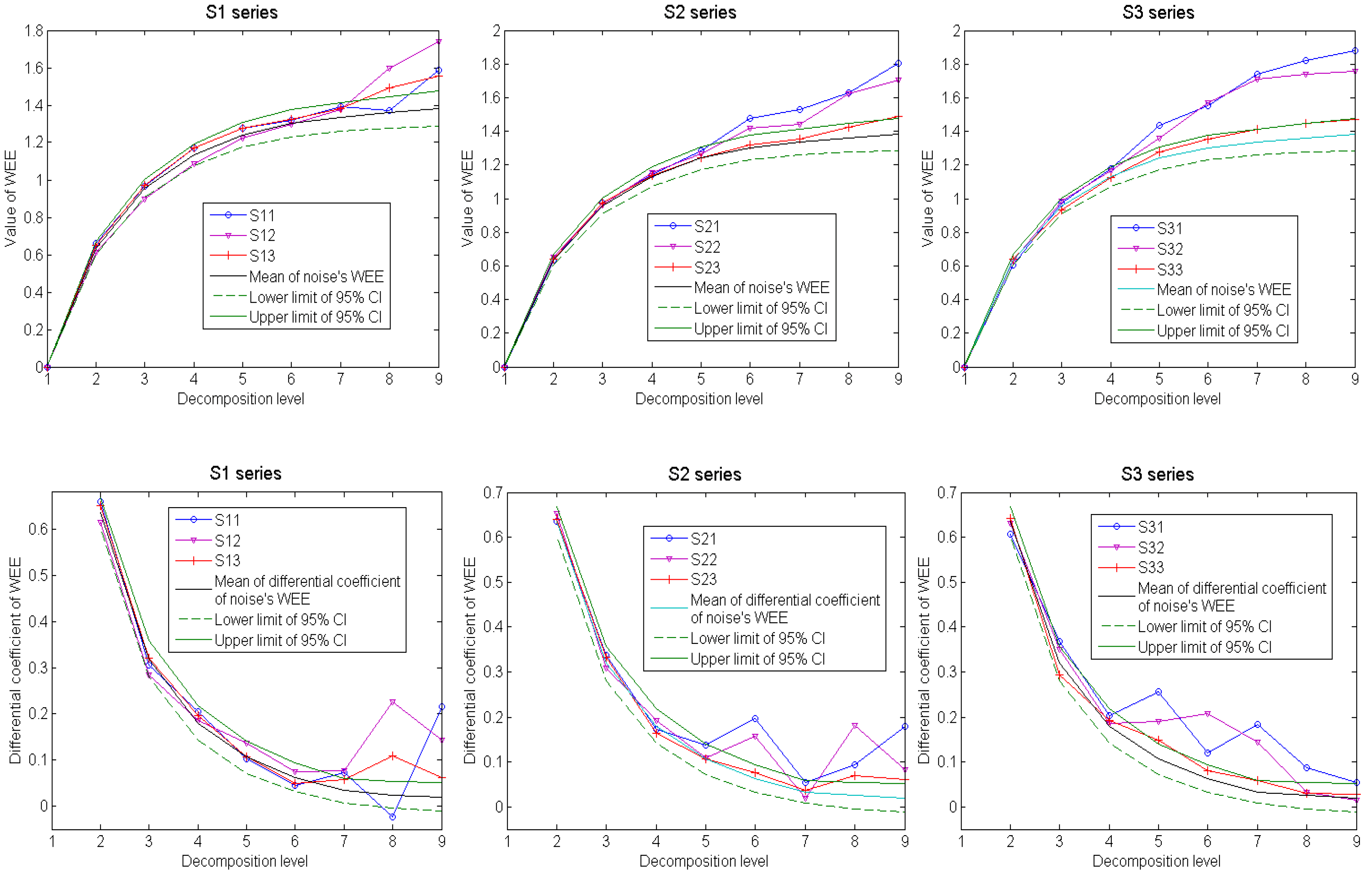
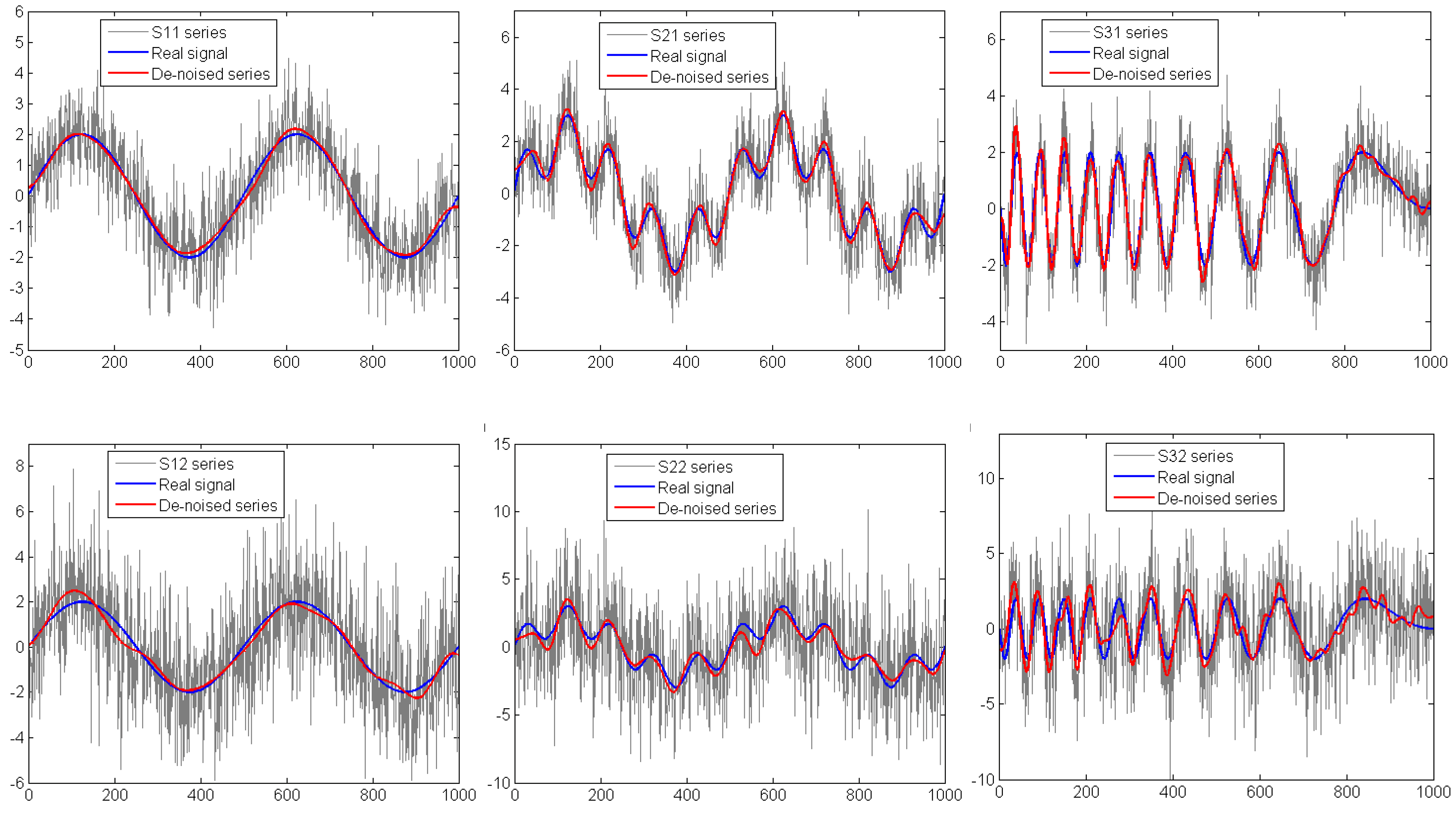
3.1. Synthetic Series Analysis

Three types of synthetic series, which include different real signals and different noise contents, were generated by the Monte-Carlo method. The real signals in them are presented in Figure 4. Concretely, the series S1 have a period of 500, and the series S2 have two periods of 200 and 500; whereas the series S3 have a ramped period. In addition, their auto-correlation characteristics and the true signal-to-noise ratios (SNRs) are presented in Table 1.

Table 1. The lag-1 autocorrelation coefficient (R₁), lag-2 autocorrelation coefficient (R₂) and the signal-to-noise ratio (SNR) of three types of synthetic series used in this paper.

Characters		S1			S2			S3
	S11	S12	S13	S21	S22	S23	S31	S32	S33
R1	0.666	0.326	0.083	0.714	0.212	0.062	0.681	0.234	0.051
R2	0.663	0.343	0.067	0.710	0.216	0.025	0.671	0.260	0.006
True SNR	7.117	−7.440	−25.855	8.352	−12.175	−32.097	6.751	−12.972	−32.192

Table 1. The lag-1 autocorrelation coefficient (R₁), lag-2 autocorrelation coefficient (R₂) and the signal-to-noise ratio (SNR) of three types of synthetic series used in this paper.

Characters		S1			S2			S3
	S11	S12	S13	S21	S22	S23	S31	S32	S33
R1	0.666	0.326	0.083	0.714	0.212	0.062	0.681	0.234	0.051
R2	0.663	0.343	0.067	0.710	0.216	0.025	0.671	0.260	0.006
True SNR	7.117	−7.440	−25.855	8.352	−12.175	−32.097	6.751	−12.972	−32.192

Each of the nine synthetic series is analyzed by the improved method using “coif5” wavelet. Their calculated WEE and D(WEE) curves are depicted in Figure 3. Considering that the analytic results of the complexities of various noises are just the same, the normally distributed noise is used here and the 95% confidence interval (CI) is estimated.

Figure 3. Values of wavelet energy entropy (WEE) and differential coefficient of WEE (D(WEE)) of three types of synthetic series obtained by using different decomposition levels (DLs), where the 95% confidence intervals (CIs) of noise’s WEE and D(WEE) are considered.

Figure 3. Values of wavelet energy entropy (WEE) and differential coefficient of WEE (D(WEE)) of three types of synthetic series obtained by using different decomposition levels (DLs), where the 95% confidence intervals (CIs) of noise’s WEE and D(WEE) are considered.

The results in Figure 3 first indicate that the D(WEE) results as a whole are much better and more convincing than those of WEE, therefore the following analysis is mainly based on the former. It shows that the chosen de-noising DLs for the three types of synthetic series are different. Because the degrees of noise contamination of the S11, S21 and S31 series are the least (the corresponding SNR values are 7.117, 8.352 and 6.751, respectively), the appropriate DLs can be accurately chosen by analyzing them. Concretely, considering the series S1, the D(WEE) values of the S11 and S12 series under the DLs from 2 to 6 fall within the 95% CI and are close to those of noise, but those under the DL7 exceed the 95% CI; as for series S2, the D(WEE) values of the S21 and S22 series under the DL6 obviously exceed the 95% CI; as for series S3, the D(WEE) values of S31 and S32 series under the DL5 obviously exceed the 95% CI; therefore the chosen DLs for de-noising them are 6, 5 and 4 respectively, and the de-noising results are depicted in Figure 4. Moreover, it shows that as the SNR values decrease, the noise contents in the synthetic series increase, thus it becomes more and more difficult to choose the appropriate DL. For instance, the D(WEE) value of S13 series under DL7 is close to the upper limit of 95% CI; the D(WEE) value of S23 series under the DL6 falls within the 95% CI and is close to that of noise; the D(WEE) value of S33 series under the DL5 just slightly exceeds the 95% CI; thus the appropriate DLs cannot be accurately chosen based on these results.

Figure 4. Three types of synthetic series used in this paper and their de-noising results.

Figure 4. Three types of synthetic series used in this paper and their de-noising results.

In addition, it demonstrates that if we use “extreme” to compare the D(WEE) difference between noisy series and noise, the applicability of the method of choosing DLs proposed in [23] would be restricted to a much smaller range, and the analytical results would be inaccurate when the studied series is too badly noise-contaminated; for the S32 series example, its D(WEE) value under the DL5 obviously falls outside the 95% CI, although it is not an extreme, so the DL4 should be chosen. Comparatively, the improved method proposed in this paper has much wider range of applicability thanks to its use of the CI to compare the WEE and D(WEE) differences between noisy series and noise, and the results obtained by using it thus become more reasonable and reliable. To sum up all the analytical results, a preliminary conclusion reached is that there is a SNR threshold which determines the applicable range of the improved method; generally, if the SNR value of a noisy series is smaller than about −25, the appropriate DL cannot be chosen anymore by using the improved method. But on the other hand, for those noisy series which are too badly noise-contaminated to identify the real signals, they generally show obviously random character but no good auto-correlation characteristics; for example, the SNR values of S13, S23 and S33 series are −25.855, −32.097 and −32.192 respectively, and the R₁ values of them are as little as 0.083, 0.062 and 0.051, respectively; therefore in the authors’ opinion, these series can be regarded as random series and their real signals need not be identified again.

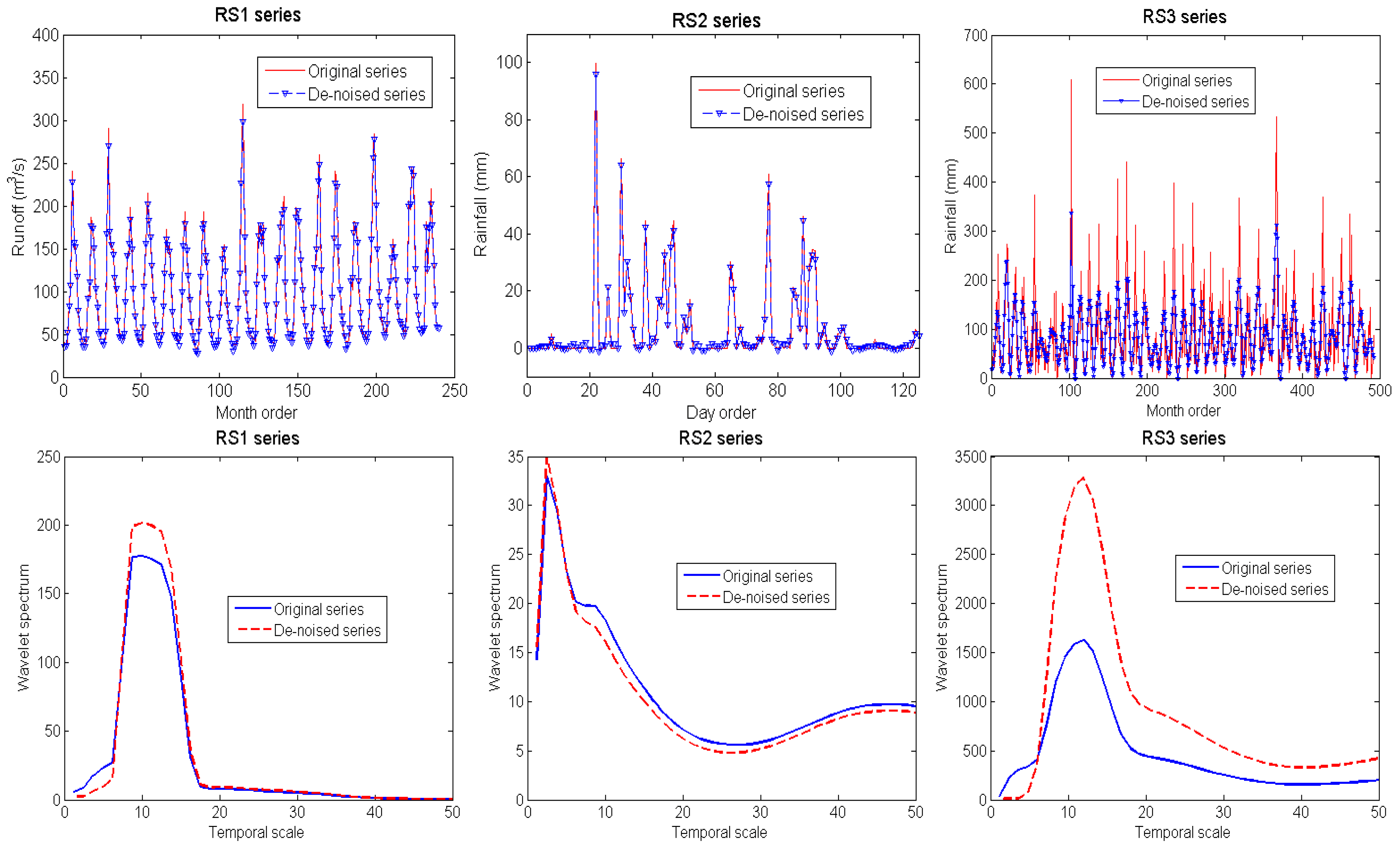
3.2. Observed Series Analysis

Three observed hydrologic series, RS1, RS2 and RS3, are analyzed here to further verify the performance of the improved DL choice method. Among them, the RS1 and RS2 series are the same as those in [23]. Specifically, RS1 monthly runoff series has a dominant period of 12 months; the RS2 daily rainfall series has no period; the RS3 presents 41-year monthly rainfall series (1961–2001) measured at the Nanjing weather station in the mid-east China, which has a dominant period of 12 months. The three observed series are analyzed by using the “dmey”, “db6” and “db10” wavelets respectively. Their WEE and D(WEE) curves are depicted in Figure 5.

Figure 5. Values of wavelet energy entropy (WEE) and differential coefficient of WEE (D(WEE)) of three observed series obtained by using different decomposition levels (DLs), where the 95% confidence intervals (CIs) of noise’s WEE and D(WEE) are considered.

Figure 5. Values of wavelet energy entropy (WEE) and differential coefficient of WEE (D(WEE)) of three observed series obtained by using different decomposition levels (DLs), where the 95% confidence intervals (CIs) of noise’s WEE and D(WEE) are considered.

Then, they are de-noised by the WTD method proposed in [13] using the chosen DLs, and the results are presented in Figure 6, in which the wavelet variance curves of original and de-noised series are also included.

Figure 6. De-noising results of three observed series by using the chosen decomposition levels (DLs) (upper), and their wavelet variance curves (lower).

Figure 6. De-noising results of three observed series by using the chosen decomposition levels (DLs) (upper), and their wavelet variance curves (lower).

Their calculated SNR values are 26.768, 48.550 and −0.594, respectively. The results in Figure 5 indicate that for the RS1 series, its sub-signals under the first two DLs are composed of noise, but its WEE and D(WEE) under the DL3 obviously exceed the 95% CI, which corresponds to its dominant period of 12 months; as for the RS2 series, it mainly reflects the daily rainfall in the rainy season in 2003 and thus has no obvious periodic characteristics, and its sub-signals under the first five DLs are mainly composed of noise, whereas the details and approximations wavelet coefficients under the DL6 reflect its trend; as for the RS3 series, its sub-signals under the first two DLs are mainly composed of noise, but its WEE, especially D(WEE), under the DL3 exceeds the 95% CI, which also corresponds to its dominant period of 12 months. Therefore, the chosen DLs for de-noising them are 2, 5 and 2, respectively. Moreover, analytical results in Figure 6 show that: (1) the original RS1 and RS2 series and their de-noised series are similar because just a little noise is included, whereas the RS3 series and its de-noised series show obvious differences, because it includes much noise and has the small SNR value of −0.594; (2) because the noise is reduced from original series, the wavelet variance curves of de-noised series are smoother than those of original series, especially those under small temporal scales, by which the real characteristic of series are much easier to be revealed; (3) analytical results of the three observed series also demonstrate the limitation of using “extreme” to compare the D(WEE) difference between noisy series and noise, as stated in [23]; for the RS3 series example, its D(WEE) under the DL3 is not an extreme but obviously exceeds the 95% CI, so the chosen DL for de-noising RS3 series should be DL2. In conclusion, the chosen DLs for analysis of the three observed series agree well with their hydrologic deterministic mechanisms respectively, thus we deem that the results are reliable. Moreover, these analytic results also manifest that the improved DL choice method has much wider applicable range, comparatively.

4. Conclusions

The choice of decomposition level is a key issue which in practice influences the effectiveness of the WTD method. In this paper, we have quantified the criterion for judging the difference of WEE and D(WEE) between noisy series and noise by taking the uncertainty into account, and then improved the DL choice method proposed in [23]. Analytical results of both synthetic and observed series have verified the performance of the improved method, and also demonstrated its much wider applicability range. In the authors’ opinion, more accurate DLs can be chosen by using the improved method, based on which the de-noising results of series can also be improved. Nevertheless, further studies using more data series with different characteristics from other domains are required to strengthen the preliminary conclusion about the wide applicability of the improved method.

References

1. Alexander, M.E.; Baumgartner, R.; Summers, A.R.; Windischberger, C.; Klarhoefer, M.; Moser, E.; Somorjai, R.L. A wavelet-based method for improving signal-to-noise ratio and contrast in MR images. Magn. Reson. Imag. 2000, 18, 169–180. [Google Scholar] [CrossRef]
2. Hrachowitz, M.; Soulsby, C.; Tetzlaff, D.; Dawson, J.J.C.; Dunn, S.M.; Malcolm, I.A. Using long-term data sets to understand transit times in contrasting headwater catchments. J. Hydrol. 2009, 367, 237–248. [Google Scholar] [CrossRef]
3. Sang, Y.F.; Wang, D.; Wu, J.C.; Zhu, Q.P.; Wang, L. The relation between periods’ identification and noises in hydrologic series data. J. Hydrol. 2009, 368, 165–177. [Google Scholar] [CrossRef]
4. Wang, D.; Singh, V.P.; Zhu, Y.S.; Wu, J.C. Stochastic observation error and uncertainty in water quality evaluation. Adv. Water Resour. 2009, 32, 1526–1534. [Google Scholar] [CrossRef]
5. Khan, T.; Ramuhalli, P.; Zhang, W.G.; Raveendra, S.T. De-noising and regularization in generalized NAH for turbomachinery acoustic noise source reconstruction. Noise Contr. Eng. J. 2010, 58, 93–103. [Google Scholar] [CrossRef]
6. Torrence, C.; Compo, G.P. A practical guide to wavelet analysis. Bull. Amer. Meteorol. Soc. 1998, 79, 61–78. [Google Scholar] [CrossRef]
7. Percival, D.B.; Walden, A.T. Wavelet Methods for Time Series Analysis; Cambridge University Press: Cambridge, UK, 2000. [Google Scholar]
8. Labat, D. Recent advances in wavelet analyses: Part 1. A review of concepts. J. Hydrol. 2005, 314, 275–288. [Google Scholar] [CrossRef]
9. Donoho, D.H. De-noising by soft-thresholding. IEEE Trans. Inform. Theor. 1995, 41, 613–617. [Google Scholar] [CrossRef]
10. Natarajan, B.K. Filtering random noise from deterministic signals via data compression. IEEE Trans. Signal Process. 1995, 43, 2595–2605. [Google Scholar] [CrossRef]
11. Kazama, M.; Tohyama, M. Estimation of speech components by AFC analysis in a noisy environment. J. Sound Vib. 2001, 241, 41–52. [Google Scholar] [CrossRef]
12. Elshorbagy, A.; Simonovic, S.P.; Panu, U.S. Noise reduction in chaotic hydrologic time series: Facts and doubts. J. Hydrol. 2002, 256, 147–165. [Google Scholar] [CrossRef]
13. Sang, Y.F.; Wang, D.; Wu, J.C.; Zhu, Q.P.; Wang, L. Entropy-based wavelet de-noising method for time series analysis. Entropy 2009, 11, 1123–1147. [Google Scholar] [CrossRef]
14. Coifman, R.; Wickerhauster, M.V. Entropy based algorithms for best basis selection. IEEE Trans. Inform. Theor. 1992, 38, 713–718. [Google Scholar] [CrossRef]
15. Berger, J.; Coifman, R.D.; Goldberg, M.J. Removing noise from music using local trigonometric bases and wavelet packets. J. Audio Eng. Soc. 1994, 42, 808–818. [Google Scholar]
16. Schaefli, B.; Maraun, D.; Holschneider, M. What drives high flow events in the Swiss Alps? Recent developments in wavelet spectral analysis and their application to hydrology. Adv. Water Resour. 2007, 30, 2511–2525. [Google Scholar] [CrossRef]
17. Jansen, M.; Bultheel, A. Asymptotic behavior of the minimum mean squared error threshold for noisy wavelet coefficients of piecewise smooth signals. IEEE Trans. Signal Process. 2001, 49, 1113–1118. [Google Scholar] [CrossRef]
18. Jansen, M. Minimum risk thresholds for data with heavy noise. IEEE Signal Process. Lett. 2006, 13, 296–299. [Google Scholar] [CrossRef]
19. Dimoulas, C.; Kalliris, G.; Papanikolaou, G.; Kalampakas, A. Novel wavelet domain Wiener filtering de-noising techniques: application to bowel sounds captured by means of abdominal surface vibrations. Biomed. Signal Process. Contr. 2006, 1, 177–218. [Google Scholar] [CrossRef]
20. Bruni, V.; Vitulano, D. Wavelet-based signal de-noising via simple singularities approximation. Signal Process. 2006, 86, 859–876. [Google Scholar] [CrossRef]
21. Chanerley, A.A.; Alexander, N.A. Correcting data from an unknown accelerometer using recursive least squares and wavelet de-noising. Comput. Struct. 2007, 85, 1679–1692. [Google Scholar] [CrossRef]
22. Box, G.E.P.; Jenkins, G.M.; Reinsel, G.C. Time Series Analysis, Forecasting and Control; Prentice-Hall: Saddle River, NJ, USA, 1994. [Google Scholar]
23. Sang, Y.F.; Wang, D.; Wu, J.C. Entropy-based method of choosing the decomposition level in wavelet threshold de-noising. Entropy 2010, 6, 1499–1513. [Google Scholar] [CrossRef]
24. Chui, C.K. An Introduction to Wavelets; Academic Press: Boston, MA, USA, 1992; Volume 1. [Google Scholar]
25. Jaynes, E.T. Information theory and statistical mechanics. Phys. Rev. 1957, 106, 620–630. [Google Scholar] [CrossRef]