Article

Statistical Information and Uncertainty: A Critique of Applications in Experimental Psychology

Department of Experimental Psychology, University of Cambridge, Cambridge, CB2 3EB, UK
Entropy 2010, 12(4), 720-771; https://doi.org/10.3390/e12040720
Submission received: 11 February 2010 / Revised: 10 March 2010 / Accepted: 1 April 2010 / Published: 7 April 2010
(This article belongs to the Special Issue Complexity of Human Language and Cognition)

Abstract

:
This paper presents, first, a formal exploration of the relationships between information (statistically defined), statistical hypothesis testing, the use of hypothesis testing in reverse as an investigative tool, channel capacity in a communication system, uncertainty, the concept of entropy in thermodynamics, and Bayes’ theorem. This exercise brings out the close mathematical interrelationships between different applications of these ideas in diverse areas of psychology. Subsequent illustrative examples are grouped under (a) the human operator as an ideal communications channel, (b) the human operator as a purely physical system, and (c) Bayes’ theorem as an algorithm for combining information from different sources. Some tentative conclusions are drawn about the usefulness of information theory within these different categories. (a) The idea of the human operator as an ideal communications channel has long been abandoned, though it provides some lessons that still need to be absorbed today. (b) Treating the human operator as a purely physical system provides a platform for the quantitative exploration of many aspects of human performance by analogy with the analysis of other physical systems. (c) The use of Bayes’ theorem to calculate the effects of prior probabilities and stimulus frequencies on human performance is probably misconceived, but it is difficult to obtain results precise enough to resolve this question.

1. Introduction

The concept of statistical information has entered psychological theory through three, distinct, routes. The first point of entry was a paper by Miller and Frick [1] that introduced Shannon’s [2] “A mathematical theory of communication” to a psychological audience. Garner (see p. 8 et seq. [3]) has charted the extraordinary and explosive impact that those ideas immediately had within psychology. Shannon’s theory suggested to psychologists that the human operator was functionally an ideal communication channel of limited capacity, with limitations on human performance deriving directly from that limited capacity. There were conferences on both sides of the Atlantic devoted to explorations of this idea [4,5,6,7,8,9] and, to many psychologists, this was information theory (and still is; e.g., [10]). This is unfortunate because Shannon’s theory is but one application of a much more general theory of statistical information, as I shall explain, and ‘information’ is used here in that more general sense. Shannon much preferred to describe his work as ‘communication theory’.
The second point of entry was through signal detection. Without using the label ‘information’, Tanner and Swets [11] transposed the “Theory of signal detectability” [12] into sensory discrimination, and the “Theory of signal detectability” stands in a direct line of intellectual descent from the Neyman-Pearson Lemma [13,14]. Signal detection is an application of information theory because of the technical foundations upon which operating characteristics are calculated. Given any statistical decision problem—the detection of a brief tone in a background of noise is one such—the optimum decision rule is to calculate the likelihood ratio with respect to the two alternatives and choose one or the other according as the likelihood ratio exceeds, or falls short, of some fixed value. Because independent probabilities multiply, log likelihood ratios add and log likelihood ratio is an information function. Given that the output of information can be measured (and estimation of the operating characteristic is exactly that), signal detection—more precisely, the theory of the ideal observer [15,16]—provides a calculus for tracking the passage of information through the human observer.
The third point of entry is encapsulated in the paper by Edwards, Lindeman, and Savage [18] on Bayesian statistical inference, but Bayes’ theorem had entered psychological theory earlier than that. One earlier example is the calculation by Green [19] of the optimum placement of the criterion in the normal, equal variance, signal detection model. This also is ‘information theory’ because the prior probability of a signal and the actual waveform presented are both sources of information about the likely occurrence of a signal. Bayes’ theorem specifies the optimum combination of the information from those two sources and provides a calculus for prior probabilities in all applications.
Notwithstanding that within psychology these three traditions have evolved in near-complete independence from each other, their intellectual foundations are closely related. In fact, their intellectual foundations are closely related also to the theory of testing statistical hypotheses, a technique that every psychologist uses at some time or other, and to the concept of entropy in thermodynamics, which has been invoked in a psychological context by Norwich [20]. The first task of this account is to bring out these interrelationships as simply as possible.
To summarize what follows:
  • In each psychological application a function of probability is sought that will be additive over independent events. Since independent probabilities multiply, that function has to be logarithmic.
  • The transmission of information effects a decrease in a potential (in the physical scientist’s sense of that term). Uncertainty and entropy are potential functions from which information is derivative.
  • There are a number of different information functions involved both in the testing of statistical hypotheses and in the various applications of information theory in psychology. The choice between them depends on the question of interest. Uncertainty and entropy are potential functions for one particular information function, specifically the function that measures ‘amount of message’ in a communication channel or work done on a closed physical system, though this same function appears in other contexts as well.
I examine a number of applications, some successful, others misconceived, with a view to some general conclusions, how the idea of information might profitably be exploited and what mistakes need to be guarded against. Some of those applications are recent, pointing to a possible revival of interest in information theory amongst experimental psychologists. Although the detailed expression of the mathematical arguments may look different in different applications, they represent a common core that is interpreted differently in different contexts. The commonality of the underlying ideas means that seemingly diverse theories are actually saying the same thing. There are therefore certain equivalences to be recognized and from that recognition there follow some tentative conclusions how information theory may best be applied in experimental psychology. The inspiration underlying this account is a belief that information theory, correctly applied, provides a powerful technique for investigating and analyzing human performance of all kinds, but a technique that psychologists have, as yet, scarcely begun to exploit.
The exploration of this complex of ideas could begin from any of a number of different starting points. I choose to start with the formal problem of the efficient testing of statistical hypotheses, because it is a part of so many psychologists’ professional expertise.

2. Information and Uncertainty

Suppose I do an experiment and record a matrix of data X. Because this particular configuration of data plays a pivotal role in the arguments that follow, I reproduce, as an example in Table 1, one set of data from Experiment 4 by Braida and Durlach [21]. In this experiment 1 kHz tones of various intensities were presented for 0.5 s, one at a time, and the subject asked to identify each one in turn. The matrix in Table 1 shows the number of times each stimulus magnitude was presented and each identification made. But I emphasize that the present argument applies to any experiment and any matrix of data will do.
Suppose I have a particular hypothesis about my experiment. Call that hypothesis H1. It is not meaningful to ask whether H1 fits my data absolutely, but I can ask whether it fits better than some other hypothesis H0. The Neyman-Pearson Lemma [13] tells us that the optimum statistic for distinguishing H1 from some other state of nature (H0) is the likelihood ratio
λ = P ( X | H 1 ) / P ( X | H 0 )
Choose a constant k. If λ > k, then, the data X are more than k times as likely under H1 as under H0. The choice of k sets the decision criterion; λ as test statistic makes the most efficient use possible of the data.
Table 1. Absolute identification of 1 kHz tones with 2 dB spacing of stimulus values from Braida and Durlach [21, Experiment 4, Subject 7]. (From “Statistical information, uncertainty, and Bayes’ theorem: Some applications in experimental psychology” by D. Laming. In Benferhat, S. and Besnard, P. (Eds.), Symbolic and Quantitative Approaches to Reasoning with Uncertainty (Lecture notes in Artificial Intelligence; Berlin: Springer-Verlag, 2001, Volume 2143, p. 636. © Springer-Verlag, 2001. Reproduced by permission).
Stimuli (dB)Responses (dB)
68707274767880828486
681203781000000
7033744215000000
7284776331020000
7408387348101000
7601943108459000
780019617736310
800000748582910
820000053874381
8400000162511529
860000000332123
If my experiment is not sufficiently decisive, I can repeat it to obtain two independent data matrices, X1 and X2. Then, analyzing these two replications together,
λ = P ( X 1 & X 2 | H 1 ) / P ( X 1 & X 2 | H 0 ) = [ P ( X 1 | H 1 ) / P ( X 1 | H 0 ) ] [ P ( X 2 | H 1 ) / P ( X 2 | H 0 ) ]
because independent probabilities multiply. Taking logarithms in Equation 2,
ln   λ = ln [ P ( X 1 | H 1 ) / P ( X 1 | H 0 ) ] + ln [ P ( X 2 | H 1 ) / P ( X 2 | H 0 ) ]
and the expression splits into two independent parts, one for each replication of the experiment. Accordingly, it is convenient to define
ln   λ = ln [ P ( X | H 1 ) / P ( X | H 0 ) ]
to be the information in the data matrix X in favor of hypothesis H1 and against H0 (see p. 5 [23]). There are two points to note:
(i)
The information defined in Equation 4 is a property of the data matrix X. Since likelihood ratio is the most efficient use of the data possible, there is no possibility of improving on the discrimination afforded by λ as test statistic. Kullback (see p. 22 [23]) expresses this in a fundamental theorem, “There can be no gain of information by statistical processing of data.”
(ii)
Information (Equation 4) is defined relative to two hypotheses, H0 and H1. Change those hypotheses, that is, change the question of interest, and the value of the test statistic changes as well. Information is information about something. Data is absolute, but information is relative to the two hypotheses to be distinguished.
Divergence. One quantity that will be repeatedly useful is the divergence of the discrimination (see p. 6 [23]). This is the mean information in favor of H1 when H1 is true plus the mean information in favor of H0 when H0 is true; that is,
Divergence = E { ln [ P ( X | H 1 ) / P ( X | H 0 ) ] | H 1 } + E { ln [ P ( X | H 0 ) / P ( X | H 1 ) ] | H 0 }
It measures, for example, the extent to which a single two-alternative forced-choice trial discriminates between two alternative stimuli or two states of nature.

2.1. Testing Statistical Hypotheses

The Neyman-Pearson Lemma has been introduced above with respect to two particular, but unspecified, hypotheses and it will help to explain at once how this formulation is related to the general practice of testing statistical hypotheses. Commonly H0 is a particular simple hypothesis (the hypothesis under test) and H1 is all the other possible states of nature bundled together (the alternative hypothesis). The Neyman-Pearson Lemma is still applicable when H1 is a compound hypothesis, except that there are usually some parameters whose values are unspecified and that need to be estimated from the data. If H0 is a special case of H1 (some otherwise free parameters are set to zero or set to be equal to each other) and the remaining parameter values are substituted by their maximum likelihood estimates, then the statistic 2 ln λ is distributed asymptotically as χ2 [24]; that is to say, the approximation of the actual distribution of the test statistic by χ2 becomes increasingly accurate as the volume of data increases. Most parametric statistical tests (the analysis of variance, for example) fall out of this formulation [23], simply by inserting appropriate hypotheses H0 and H1 in Equation 4 and calculating the distribution of the test statistic when H0 obtains. The best-known exception is Pearson’s X2. In many cases a more accurate formulation of the distribution is known, and the statistical tests in practical use are those tests for which it is feasible to calculate the distribution of the statistic when H0 is true.
As an example, suppose that H0 asserts that the row and column classifications in Table 1 are independent; (this is manifestly false, but it is the H0 for which the distribution of ln(likelihood-ratio) is readily calculable). The arguments that follow repeatedly focus on data matrices like that in Table 1, so let pij stand for the probability of some particular combination of stimulus (i) and response (j); let pi. be the marginal probability of stimulus i (that is, the sum Σj pij, with the dot replacing the index of summation), and p.j the marginal probability of response j. Then, the hypothesis of independence of the row and column classifications is
H 0 :   p i j = p i . × p . j
while the alternative hypothesis
H1: ∑ij pij = 1
allows the probabilities of individual cells (pij) to assume any set of values that sum to unity. Note that any set of {pij} specified by H0 is a possible set of probabilities under H1; H0 is a special case of H1.
Suppose stimulus i is presented and response j occurs. The probability ratio attaching to that datum is [pij /pi.p.j], because, under H0, stimulus and response are independent (their joint probability is pi.p.j). the mean information in favor of H1 from a single trial, averaged over all combinations of stimulus and response (probability under H1 is pij), is therefore
i j p i j ln [ p i j / p i . p . j ]
In practice, the unknown probabilities (pij, pi., and p.j) are estimated from the data and the resultant statistic gives us Wilkes’ [25] likelihood-ratio test of independence in two-way contingency tables.

2.2. Inverting the Test Procedure

To summarize the generic test procedure succinctly, there are two hypotheses H0 and H1 and a body of data X. The distribution of X under both hypotheses is known and λ = P ( X | H 1 ) / P ( X | H 0 ) can be calculated. If λ exceeds some criterion value k, H1 is selected as the most likely state of nature, otherwise H0. This procedure represents the most efficient use of the information in X with respect to the two hypotheses H0 and H1.
Now turn that procedure inside out to address this problem. There is a physical system (a human observer) and experimental evidence to suggest that the transmission of information (e.g., discrimination between sensory stimuli) is less than optimum. Why so? Conduct this experiment: There are two stimuli; one is simply a sample of noise (H0) and the other a sample of the same noise with a signal superimposed (H1). One or the other stimulus is presented and the observer asked to identify it; in fact, he or she is asked to assign each trial to one of six categories of progressively increasing confidence that it was signal-plus-noise rather than noise alone that was presented cf. [26]. That experiment is repeated hundreds of times to generate an estimate of the operating characteristic (and, to pre-empt confusion, I remark that the hundreds of trials taken together comprise one conventional signal-detection experiment, but that each trial is here treated as a separate ‘experiment’, and the hundreds of trials are needed to provide a sufficiently accurate estimate of its power function).
There are models of the noise and of the superimposed signal [12;16, Chapter 6], from which the distribution of information at the physical level of description, in favor of signal-plus-noise and against noise alone, can be calculated. There is a model of the operating characteristic fitted to the data, from which the distribution of information expressed in the responses can be estimated (see pp. 98–103 [27]), as explained below. ‘Inverting the test procedure’ means comparing the two to discover how the ‘data’ (the physical stimulus) has been ‘analyzed’ (processed by the sensory pathway).
The operating characteristic is a relation between α, the probability of a false positive, and β, the probability of a correct detection in Figure 1. That relation can be formulated as a pair of parametric equations:
P ( False positive ) =   α ( x ) P ( Correct detection ) =   β ( x ) }
Since 0 ≤ α, β ≤ 1, α(x) and β(x) can be interpreted as cumulative probability distribution functions with respect to x. For convenience, suppose them to be differentiable. Then the probability ratio associated with a given value of x is
λ=dβ(x)/dα(x)
and this is the gradient of the operating characteristic at the point (α, β) in Figure 1. The information, in favor of signal-plus-noise and against noise alone in the variable x is ln λ.
The relation between α and β expressed by the parametric equations (7) is invariant under any monotone transform of the argument x. Suppose x is replaced by some transform y(x). Then
d α ( x ) / d x = [ d α ( y ( x ) ) / d y ( x ) ] [ d y / d x ]
with a similar equation for β(y). The functions α(x) and β(x) may be arbitrarily distorted by substituting y(x) for x, but the ratio
d β ( y ( x ) ) / d α ( y ( x ) ) = d β ( y ( x ) ) / d y ( x ) d α ( y ( x ) ) / d y ( x ) = [ d β ( x ) / d x ] [ d x / d y ] [ d α ( x ) / d x ] [ d x / d y ] = d β ( x ) / d α ( x )
is unchanged. In particular, the choice y = ln λ(x) expresses the operating characteristic directly in terms of information as decision variable.
Figure 1. Signal-detection operating characteristics and the gradient at a typical operating point. (From Mathematical Psychology, by D. Laming, p. 75. London: Academic Press, 1973. © Copyright Elsevier 1973. Reproduced by permission.).
Entropy 12 00720 g001
All this follows without any assumption whatsoever about the internal workings of the human observer. True, there are models of the stimuli, but these belong to the domain of physical science where theory is well–developed and reliable. A model is also needed to interpolate between the five or so data points that estimate the operating characteristic, but that is a purely empirical matter. Otherwise, turning the signal-detection paradigm inside out delivers a comparison between ‘information in’ and ‘information out’ that is model-free. It allows us to ask, absolutely: What information has been lost in transmission? Some examples will show later what can be achieved with this technique.

2.3. Channel Capacity in A Communication System

Suppose that my experiment consists of sending messages through a communication system. As in Table 1, I record the number of times message (stimulus) i is sent and received as message (response) j. Given the resultant matrix of data (X), I ask: Is this communication channel working (not necessarily perfectly, but with some degree of reliability: H1) or is the line open-circuit (that is, the message received is independent of the message sent: H0)? The appropriate statistical test is Wilkes’ [25] likelihood-ratio test of independence (above). If a single message takes T s to transmit, then
i j p i j ln [ p i j / p i . p . j ] / T
is an estimate of the mean information transmitted per second. Depending on my choice of message ensemble (that is, on the sensitivity of the design of my experiment), the mean information transmitted might take various values. But there is an upper limit, because any combination of messages sent and received under H1 (probability pij) is also possible under the hypothesis of independence (H0, probability now pi.p.j), so that the probability ratio in Formula 11 is always finite. The upper limit is achieved when the ensemble of messages to be transmitted is optimally matched to the statistical characteristics of the communication channel. this upper limit is known as the channel capacity. If the natural logarithm in Formula 11 be replaced with a logarithm to base 2 (this is common in communication theory), then a message conveying a single unit of information will distinguish perfectly between exactly two alternatives. That single unit of information is called a ‘bit’.
Shannon [2] examined a variety of communication systems. If the channel can transmit up to n symbols per second without error and if each symbol can be chosen from m alternatives, then a 1-second transmission suffices to distinguish between mn alternatives (but not more) and the channel capacity is n log2 m. More realistic is a continuous channel—that is, a channel passing a continuous waveform f(t)—perturbed by noise. If the waveform is limited to the frequency band (0, W), then the function f(t) can be reconstructed from its values at intervals of 1/2 W, and Shannon [28] describes a set of elementary functions which enable this reconstruction to be accomplished (see pp. 154–162 [16] for a simpler account). This means that T s of message through such a channel is equivalent to the transmission of 2 WT independent voltages, and the information transmitted is maximal if those voltages are normally distributed [2]. If, in addition, the average power of the signal (i.e., the mean square of the signal voltage, averaged over 1 s) is limited to P, while the noise contributes a power N, each normal variate carries information equal to log2 (P+N)/N and the channel capacity is
2 W  log 2 ( P + N N   )
In practice, the messages to be transmitted (text) are not well matched to the waveforms that a communication channel transmits. The letters in English text do not occur with equal frequencies and successive letters are not statistically independent. efficient coding requires strings of text symbols to be mapped on to segments of channel waveform of equivalent frequency of occurrence. Shannon [2] showed that, given an arbitrary message source, a system of encoding could always be found that afforded transmission at a rate arbitrarily close to the limiting capacity of the channel, though that capacity limit could never be exceeded. The limiting capacity is approached by holding long sequences of input messages in the transmitter while the appropriate channel waveform is determined.

2.4. Uncertainty [29]

Suppose I send just a single message, selected with probability pi. from a set of possible messages. Suppose this transmission is received as message j. Given an arbitrary selection of that single message, the mean information transmitted is given by Formula 6. The information transmitted is maximal when, given the message received, it is always known exactly which message was sent; that is, when the message received (j) identifies the message sent (i) uniquely. This happens when pkj = 0 for all messages k other than j, so that p i j = p . j . Canceling pij and p.j, the maximum value is then
i j p i j ln ( 1 / p i . ) = i p i . ln p i
This expression is the uncertainty of the choice of message input; at the same time, it is the maximum information that can be transmitted per trial in my experiment.
if I know that message j was received, what is the probability that it was message i that was sent? The joint probability of choosing message i to send and receiving message j is pij. Since message j is known to have been received, the relative probabilities of the different messages that might have been sent must be proportional to {p1j, p2j, … pnj}, and the absolute probability must be p i j / i p i j = p i j / p . j . Substituting this expression for pi. in Formula 13, the uncertainty (now residual uncertainty) is reduced to i    ( p i j / p . j ) ln ( p i j / p . j ) , and the average residual uncertainty over the different received messages j is
i j p i j ln ( p i j / p . j )
But
i j p i j ln ( p i j / p i . p . j ) = i p i . ln p i + i j p i j ln ( p i j / p . j )
so that the information transmitted can be represented as the difference between the initial (stimulus) uncertainty (Formula 13) and the residual uncertainty (Formula 14) conditional on the message received.
One might, for this reason, be tempted to suppose (erroneously) that uncertainty is fundamental and information derivative. But suppose the input message to be a normally distributed voltage (zero mean, variance σ2) and the output likewise, correlated ρ with the input. The information transmitted is then 1 2 ln ( 1 ρ 2 ) (see p. 8 [23]), irrespective of the value of σ2, but the input uncertainty is
1 2 ln ( 2 π σ 2 ) 1
which depends on the choice of σ2. That is, uncertainty depends on the underlying metric (which is hidden in Equation 15), but information does not. When information is calculated as a difference of uncertainties (as in Equation 15), the scale factor (σ2) drops out of the reckoning [30]. Uncertainty therefore stands in relation to information as velocity potential stands in relation to velocity in physical field theories, or voltage to current flow in an electrical circuit. Only differences in potential or voltage are physically significant.

2.5. Entropy

Many people, not least Shannon (see p. 393 [2], [31]) have commented that the expression for uncertainty (Formula 13) is of the same mathematical form as the expression for entropy in thermodynamics and have wondered what, if anything, that formal similarity signified. This is potentially important because the Second Law of Thermodynamics can be formulated in these terms: In any closed system the entropy does not decrease. That is to say, the entropy function specifies in which direction macroscopic physical and chemical reactions proceed. The following explanation relies heavily on the account of entropy by Landau and Lifshitz [32].
The position and motion of a particle in three-dimensional space can be described by six variables, the three co-ordinates x, y, and z, and their time rates of change (the velocities, x ˙ , y ˙ , and  z ˙ , although mathematicians and physicists prefer to use the momenta [mass × velocity], which confers a technical advantage). The state of a single particle (position and velocity) can therefore be represented by a single point in a six-dimensional space known as phase space. Now envisage a system comprised of n particles; these could be the molecules in a volume of an ideal gas, so that n could be very large. The state of such a system can be represented in a phase space of 6n dimensions and its evolution by a path in that phase space (and the fact that 6n might be a hideously large number is of no consequence because phase space is no more than a mathematical construction). The concern here is with a system in statistical equilibrium, which means that over a long period of time the system visits all achievable states (all reachable points in phase space) according to a stationary distribution that describes the equilibrium. One might equivalently think of a large number of parallel and independent systems simultaneously occupying different points in phase space according to that stationary distribution.
A closed physical system in statistical equilibrium remains in that equilibrium and any other closed system will naturally tend to equilibrium. So the statistical equilibrium identifies the direction in which macroscopic physical and chemical reactions are observed to proceed. A function of the system (entropy) is required that is maximal when the system is in equilibrium. In principle there are many such functions, but one particular consideration determines the mathematical expression for entropy. A system composed of a very large number of particles can be decomposed into subsystems (still containing very large numbers of particles) that, over relatively short periods of time, are quasi-independent of each other. Each subsystem moves in its own hyper-plane of the phase space, a hyper-plane generated by that subset of the 6n dimensions that describes the position and motion of the particular particles in the subsystem. The probability (density) that the entire system is at a given point in phase space is therefore the product of the probabilities that the separate subsystems are at the corresponding points in their hyper-planes of phase space; that is, using ρ to denote a density,
ρ = ∏i ρ i,
where the product extends over the different subsystems. At the same time, it is desirable that the entropy function of a combination of systems should be chosen so that the entropy of a combination of systems is equal to the sum of their constituent entropies, and this is achieved by taking logarithms in Equation 17. Consequently entropy is defined to be the expectation of log probability density; i.e.
Entropy = ln ρ     d ρ
where the integral extends over the entire phase space.
In the case that the equilibrium distribution is discrete, Equation 18 reduces to Formula 13 above. In both cases the formula describes a potential that is changed either by work done on a physical system (according to the second law of thermodynamics) or by information transmitted (through a communication system). The similarity arises, first, because independent probabilities multiply. A function that is additive over independent probabilities therefore has to be logarithmic. Second, a multinomial distribution {p1, p2, … pn} can be decomposed into a conditional distribution {p1/(p1+p2), p2/(p1+p2)} occurring with probability (p1+p2), and an unconditional distribution {(p1+p2), p3, … pn}. A function decomposing in parallel has to have the form (13) (see Theorem 2.4.7 [33]). The similarity between uncertainty and entropy simply reflects the additivity of information transmitted on the one hand and work done on the other. The mathematics is the same, but is interpreted differently in the two cases.
This mathematical argument may be applied to any context. The question whether an argument is valid depends on the mathematics, not on the interpretation; but the question what such an argument means, given that it is valid, depends on the interpretation and that interpretation must match the context to which the mathematics is applied. There needs to be a correspondence between the assumptions of the mathematical argument and the context to which it is applied; and that correspondence determines how the argument is to be interpreted. I illustrate this with one example here and others below.
Sinusoidal gratings. Envisage a visual experiment with grating stimuli. The stimulus is, physically speaking, a Poisson process with density (luminance) varying sinusoidally across the face of the grating, as
L(u) = L0{1+C cos 2πgu}
where C is the contrast of the grating and g is its wavenumber with respect to a spatial co-ordinate u (e.g., Figure 8.3 [34]). For each small area and duration δ(AT) of the stimulus, the input is a Poisson variable with parameter λ = L(u)δ(AT). Formula 13 with respect to the Poisson distribution pk = eλn/n! may be expressed as
0 p i ln p i = 0 e λ λ n n ! [ ( λ λ 0 ) + n ln ( λ / λ 0 ) λ 0 + n ln λ 0 ln n ! ] = ( λ λ 0 ) λ ln ( λ / λ 0 ) 0 e λ λ n n ! [ λ 0 + n ln λ 0 ln n ! ]
where λ0 denotes the Poisson density for the mean luminance L0 (i.e., for a grating with zero contrast). The term in square brackets under the summation sign is therefore independent of u, and when Equation 20 is integrated over a complete cycle of the modulation, contributes a constant term only. The other two terms in Equation 20 may be written as
L 0 C  cos  2 π g L 0 { 1 + C  cos  2 π g } ln { 1 + C  cos  2 π g } L 0 C  cos  2 π g L 0 { 1 + C  cos  2 π g } C  cos  2 π g
which integrates, again over a complete cycle of the modulation, to –½L0C2. In short, the value of Formula 13 for this grating stimulus is –½L0ATC2+ a constant. It is maximal when C = 0.
During passage through the optic media, the visual stimulus suffers a small amount of scatter and also some diffraction at the pupil. This process could be modeled as a locally random re-distribution of quanta across the face of the grating, leading to some reduction at the peaks and some filling in of the troughs. Some of the quanta will be absorbed in the retina and give rise to perturbations of cellular potential. Those perturbations suffer similar random relocations in the course of lateral transmission from receptors to ganglion cells. The neural connections which effect this transmission are, of course, quite determinate, but, because the retina is moving in relation to the stimulus, the effect is random with respect to the stimulus domain. Both these local relocations, interpreted with respect to the domain of the physical stimulus, serve to reduce spatial modulation and thereby increase entropy. The Second Law of Thermodynamics transposes into the theorem that there can be no increase in modulation referred to the spatial domain (i.e., effective contrast) in the course of transmission through the visual pathway.
Now envisage that a sinusoidal grating is suddenly projected on to the retina. The pre-exposure field is (taken to be) a uniform field of the same space-average illuminance, so that the presentation of the grating leads to a reduction in the entropy of the visual field. That circumstance parallels the fact that the entropy of a system can be reduced only by doing work on it (Clausius’ theorem). A common everyday example is provided by a refrigerator in a kitchen. Ordinarily, the contents of the refrigerator would assume the ambient temperature of the kitchen. The interior of the refrigerator can be kept colder than that ambient temperature only by doing work to transfer heat from the interior of the refrigerator to the kitchen outside. The visual analysis of a grating stimulus is subject to the same constraint.

2.6. Bayes’ Theorem

Suppose that P(X1|H1) and P(X1|H0) in Equation 3 be replaced by prior probabilities P(H1) and P(H0). Then, writing X in place of X2,
ln   λ = ln [ P ( H 1 ) / P ( H 0 ) ] + ln [ P ( X | H 1 ) / P ( X | H 0 ) ]
in words,
Posterior information = Prior information + Information in X.
Exponentiating both sides of Equation 22,
P ( H 1 | X ) / P ( H 0 | X ) = P ( H 1 ) P ( X | H 1 ) / P ( H 0 ) P ( X | H 0 )
which is Bayes’ theorem.
Human performance is manifestly influenced by the relative frequencies of different stimuli, and the simplicity of Bayes’ theorem has long commended it as a normative model for combining prior probabilities with sensory information. But there is a problem: What values should be assigned to the prior probabilities or, alternatively, how should those values be determined? A probability is not a stimulus and cannot be presented as such. It is a property of a potentially infinite sequence of stimuli. In any realizable experiment such a sequence is presented stimulus by stimulus and human performance is adjusted, not to the sequence as a whole, but to individual stimuli, one by one. Whether such a process equates to Bayes’ theorem is an empirical matter that will be examined later.
Nevertheless, people have prior beliefs and probability theorists and philosophers and psychologists have sought to formulate the subjective values of beliefs in a manner that melds with objective probability theory. Good [35], for example, proposes a logic of statements expressing the probability that some proposition is true. While this might look like the (objective) probability attaching to a hypothesis on the basis of experimental data, it is actually an attempt to formalize the strengths of (subjective) beliefs. It leads to curious circumlocutions: Whereas most people would speak directly of the (objective) probability of an event, when Good uses such a phrase, he actually means “the probability of a proposition asserting that the event will happen or has happened.” (see p. 34 [35]).
I do not engage in the debate over subjective probabilities here; but I note that the manner in which prior and posterior probabilities are parameterized (e.g., the choice of metric of a density function), and thereby enter into calculation, is at our disposal. This choice does not arise with discrete random variables, but gives the mathematical representation of a continuous variable the character of a potential. Information, in Equation 23, is the difference between prior and posterior probabilities subject to the same parameterization and can be evaluated objectively. This has several consequences:
(i)
One cannot invoke prior probabilities in psychological theory in the same way as information.
(ii)
Although the format of significance testing appears to assign an absolute probability to H0, this is illusory. A significance test calculates the probability of the observed data if H0 were true; that probability cannot be transposed into an absolute probability of H0 without reference to an absolute prior. All that a significance test can do is assess the concordance between observation and theory.
(iii)
Since ‘probable’ is used in everyday parlance, it is natural to attempt to extrapolate the calculus of probability theory to ‘subjective probabilities’. But these are no different from beliefs of various strengths cf. [35] and beliefs have their own psychology [36, Ch. IX; 37]. There is no a priori reason why beliefs should satisfy any particular calculus.
(iv)
The use of ‘information’ in this article is specific to information derived from the analysis of empirical data. ‘Information’, of course, has many other meanings in everyday discourse and those other meanings are excluded from consideration here. Likewise the scope of ‘uncertainty’ is restricted to those potentials with respect to which information can be calculated. Other uses of ‘uncertainty’ in everyday parlance are likewise excluded.
Applications of Bayes’ theorem in psychology will be examined in due course from this standpoint.

2.7. Interim Summary

The same formal set of ideas, with only minor variation in the arguments, recurs in many different contexts. The mathematical arguments have been adapted by psychologists in different ways, not always correctly. In what follows I distinguish
(i)
applications in which the mathematical assumptions fail to match the details of the experiment;
(ii)
applications in which the experiment and the human observer taken together is treated as a purely physical system; and
(iii)
applications which use Bayes’ theorem to relate experimental performance to prior stimulus probabilities.
Finally, to summarize this introduction, Table 2 sets out some important parallels between information theory, an ideal communication system, and the psychological experiments that are to be examined in the remainder of this paper.
Table 2. Some conceptual parallels between information theory, an ideal communication system,thermodynamics, and psychological experiments.
Information theoryCommunication theoryThermodynamicsExperimental application
Message sent Stimulus
Message received Response
DataTransmission frequencies Performance data
Null hypothesisChannel open-circuit Independence
Alternative hypothesisChannel functioning, but subject to error Task completed, but with errors
Information statisticInformation transmittedWork doneMeasure of task performance
UncertaintyEntropyMaximum yield of information

3. Mathematical Theory not Matched to the Psychological Task
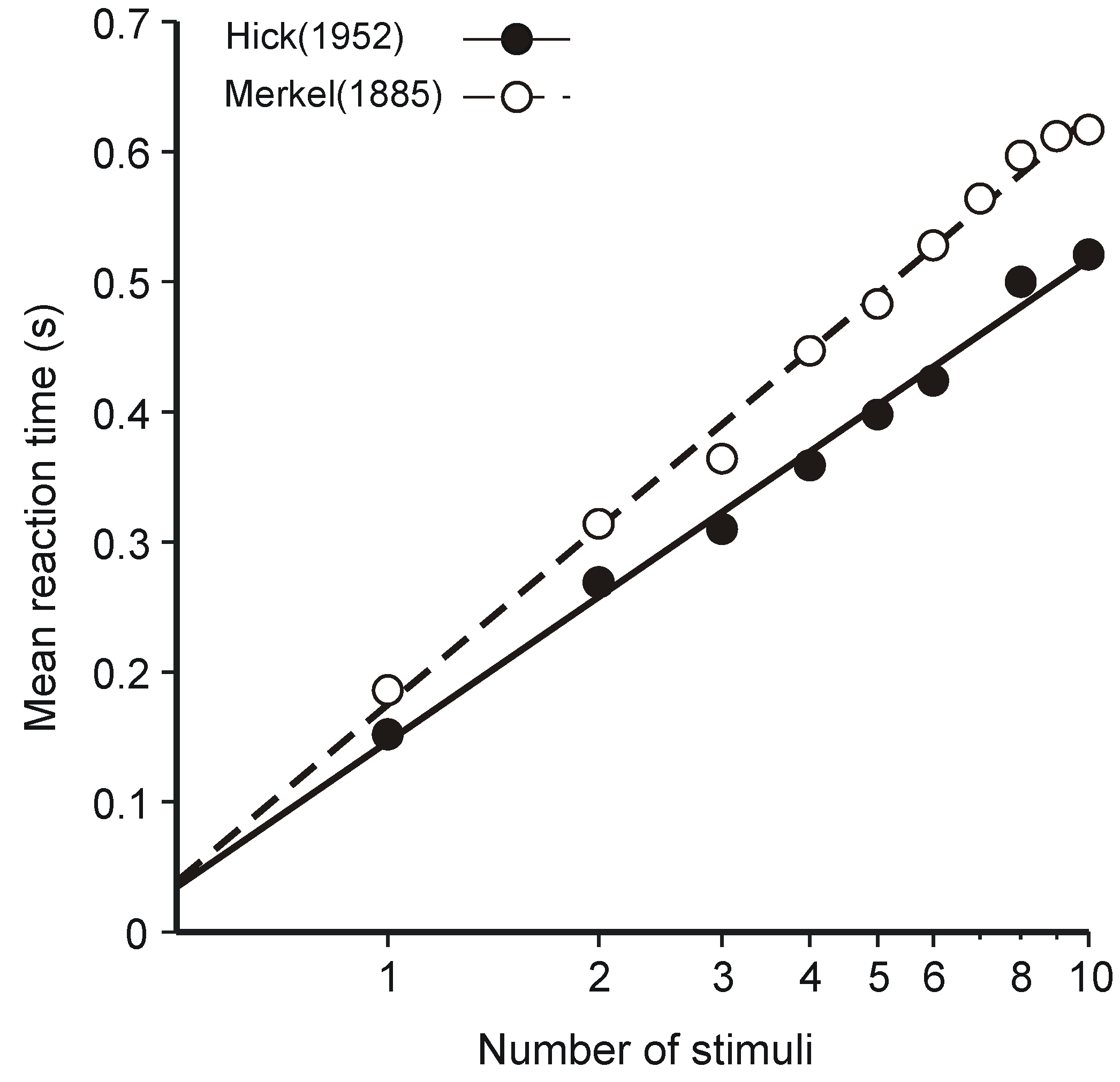
As a matter of meta-theoretic principle, it is not sufficient merely for an equation to agree with an observed result. The derivation of that equation—the assumptions on which it is based—must also be reflected in the details of the psychological experiment. In this section I examine four applications in which this principle was flouted.

3.1. Hick’s Law

There are n equally probable stimuli (pea bulbs) arranged in a “somewhat irregular circle”. The subject responds as quickly as possible with a different response depending on the stimulus. Hick [38] fit his own data and some historic data from Merkel [39] to the equation
Mean R.T. = a ln ( n + 1 )
in which the possibility of “no signal” was regarded as an (n+1)th alternative. The quality of the fit is shown in Figure 2, where the abscissa is scaled according to ln(n+1).
Figure 2. Mean choice-reaction times from Hick [38] and Merkel [39] plotted against ln(n+1). (From “Statistical information, uncertainty, and Bayes’ theorem: Some applications in experimental psychology” by D. Laming. In Benferhat, S. and Besnard, P. (Eds.), Symbolic and Quantitative Approaches to Reasoning with Uncertainty (Lecture notes in Artificial Intelligence, Volume 2143). Berlin: Springer-Verlag, 2001, p. 639. © Springer-Verlag, 2001. Reproduced by permission.).
Entropy 12 00720 g002
If pi. be put equal to 1/(n+1) in Formula 13, the stimulus uncertainty is ln(n+1), and Equation 25 is equivalent to
Mean R.T. = a (Stimulus uncertainty)
The underlying idea equates mean reaction time to the time taken to pass a message through an ideal communication system, a message with just sufficient content to specify the response. The apparent success of this relation in modeling these data was influential, above all other applications at that time, in encouraging the idea that the human operator is analogous to a communication channel operating at maximum capacity. It has given us such terms as “(channel) capacity” and “encoding”. But note the assumptions that are involved:
(i)
The human operator is functionally a communication system—that assumption is patently true and goes without saying—and
(ii)
The (human) communication system is operating at (or near) maximum capacity.
It is assumption (ii) that gives the logarithmic relation (Equation 25); assumption (i) by itself does nothing. while Hick’s data demonstrate that the time taken to respond to a stimulus depends not only on that particular stimulus, but also on what other stimuli might have been presented in its stead, it does not necessarily follow that the relationship between stimuli and reaction time is that dictated by the capacity limitation of a communication channel.
In fact, the idea will not wash. A choice-reaction experiment involves the transmission of single stimuli, one at a time, a condition that affords no opportunity for the sophisticated coding on which Shannon’s theorem depends (see pp. 18–24, esp. Figure 3 [38]). Reaction time is an actual transmission time, while Shannon’s theory applies only to the limiting rate at which a continuous stream of messages can be passed through the channel. Those messages might suffer an arbitrary delay before transmission to allow for encoding. The logarithmic formula relates to the length of encoded signal in the channel that is needed to carry the message, not to the delay it might suffer in transmission.
This mismatch between the assumptions of the mathematical theory and the circumstances of the experimental task has these consequences. First, it provides opportunities for modifications of the experiment to demonstrate incompatibility with the theory. For example, if the length of message to be encoded is increased, more sophisticated encoding is possible and performance is enhanced. That can be realized in a reaction time task by asking the subject to respond, not to the present signal (‘no-back’), but to the signal one, or two, or three places back in the presentation series. The task then more closely approximates the condition under which a communication channel can operate efficiently. but the laboratory task, on the other hand, becomes progressively, and very rapidly, more difficult. Kirchner [40] presented visual stimuli, either 6 or 12 alternative stimuli, at 1.5 s intervals; Table 3 records the percentages of correct responses by three groups of subjects. It is patent that the difficulty in this task lies in remembering which stimuli have recently been presented. The ideal communication hypothesis assumes that there is no limitation of memory, only channel capacity.
Table 3. Percentage of correct responses in the experiment by Kirchner [40].
SubjectsExperimental condition
No-backOne-backTwo-backThree-back
Sailors100.099.486.055.0
Students100.098.892.969.8
Old people99.187.351.9
Again, different reaction-time tasks reveal quite different rates of transmission (see [41]; pp. 13–14 in [42]). The rate of transmission (the constant a in Equation 25) is manifestly not a universal constant. Indeed, if the responses are relay armatures to be pressed with the finger tips and the stimuli consist of vibration of the corresponding relay armatures, then there is no increase in reaction time from two to eight alternative stimuli [43].
A second consequence of tolerating this kind of mismatch between theory and experiment is that it discourages the search for alternative explanations. For example, ln (n+1) is approximately equal to the sum 1 n + 1 r 1 , which in turn is the mean of the longest of (n+1) exponential latencies [44]. This formula fits the data in Figure 1 about as well as Equation 25 [45] and leads to a quite different range of theoretical ideas that have since been much explored in other contexts e.g. [46].

3.2. Information Transmission in Category Judgments

Experiments by various authors in the 1950s led to the then surprising conclusion that the accuracy of judgment of some continuous stimulus attribute—sound pressure level, frequency of a tone, luminance—could never exceed a limit equivalent to the use of five categories without error. Expressed in term of information transmitted, this equated to 2.3 bits, and this limit applied however many different stimulus values were presented and however many response categories were available for the participant to use. The only exceptions were experiments in which some physical comparator was available to assist judgment [47], and attributes like color and inclination [48,49,50] for which it is plausible that there is some internal comparator. In these exceptional cases the improvement in accuracy was strictly related to the additional information supplied by the comparator.
This discovery led to the idea that category judgment was also information limited (see Chapter 3 [3]), notwithstanding that the subjects in these experiments had effectively unlimited time in which to respond. This means, of course, that the limiting capacity of a hypothetical communication channel could not possibly bear on this result. Instead, it looks as though any logarithmic limit invoked the idea of channel capacity at that time, even though, as in these experiments, the limit could be expressed in other non-logarithmic ways.
Figure 3. Mean information transmitted per trial in Experiment 4 by Braida and Durlach [21]. Data for three observers.
Entropy 12 00720 g003
As a further example of this finding, Figure 3 displays the mean information transmitted per trial in Experiment 4 by Braida and Durlach ([21] cf. Table 1 above). The stimuli were ten 1 kHz tones of different amplitudes and 0.5 s duration. The observers were required to identify individual tones in isolation. In different sessions the tones were spaced at 0.25, 0.5, 1, 2, 3, 4, 5 and 6 dB intervals with the highest level always set at 86 dB. At small dB separations, identification is hampered by sensory confusion between adjacent stimuli; but, as the separation increases, the information transmitted increases to an asymptote at 1.80 to 2.00 bits for different participants, equivalent to four categories without error. I shall return to this experiment later to demonstrate a simpler formulation of this result that owes nothing at all to the idea of a limited capacity for information.

3.3. Optimal Data Selection in Wason’s Selection Task

There are four cards, each of which has a letter on one side and a number on the other. Given four cards with ‘A’, ‘K’, ‘2’, and ‘7’ uppermost, which of them need to be turned over to discover whether it is true that “If a card has a vowel on one side, it has an even number on the other”? In the early experiments only about four per cent of participants (university students) selected ‘A’ and ‘7’ [51].
Oaksford and Chater [52,53,54, pp.169–174] proposed that the subject considers these two hypotheses with respect to an imagined population of cards of which ‘A’, ‘K’, ‘2’, and ‘7’ are but a sample:
  • H0: P(vowel & odd number) = 0.
  • H1: Number (even or odd) independent of letter (vowel or consonant).
This conflicts with conventional statistical methodology which requires H0 (the rule to be tested) to be compared to all alternative states of nature, that is to
  • H2: P(vowel & odd number) ≠ 0,
and not just to the special case H1. There is therefore a surreptitious assumption that all possibilities alternative to H0 (P(vowel & odd number) = 0) and H1 (Number and letter independent) are deemed by participants to have probability zero, and this is the first respect in which this particular theory fails to match the psychological task. While the four cards can be presented as a sample from some larger population in an appropriate experimental design e.g., [55,56]; but this has not traditionally been a feature of Wason’s selection task], the surreptitious assumption has no counterpart in nature. the comparison between H0 and the particular H1 does not, therefore, generate a model of Wason’s selection task [57].
Oaksford and Chater next proposed that participants select amongst the four cards ‘A’, ‘K’, ‘2’, and ‘7’ according to the expected yield of information measured according to
i ln [ p i j / p i . p . j ]
where i indexes the hypothesis (H0 or H1) and j the choice of card. They believed that such a sampling strategy would be optimal, though Klauer [60] has shown otherwise. Formula 27 is the Shannon measure of information transmitted conditional on selecting Card j. It decomposes Formula 6 into four components corresponding to j = ‘A’, ‘K’, ‘2’, and ‘7’. If p0j : p1j = p0. : p1., then formula 27 equates to zero. So Oaksford and Chater propose that participants select among the different cards (j) according as p0j : p1jp0. : p1., that is to say, according as the proportions of even : odd or vowel : consonant differ from the average. This does, indeed, distinguish between H1 above and H0. It distinguishes equally between H1 and P(vowel & even number) = 0, P(consonant & even number) = 0 and P(consonant & odd number) = 0. These last three hypotheses are excluded from consideration solely by fiat.
A even more optimal procedure for selecting between the cards would use the divergence (Equation 5) as criterion. This measures the extent to which the underside of each card may be expected to discriminate between the hypotheses H0 and H1. Hypothesis H1 says that the frequencies of even and odd under a letter are the same for both vowel and consonant; likewise the frequencies of vowel and consonant under a number. Hypothesis H0, on the other hand, says nothing about what lies under ‘K’ or ‘2’; those cards therefore have zero divergence and should never be selected. But the divergences of ‘A’ and ‘7’, on the other hand, are infinite. It happens so because a single odd number beneath an ‘A’ or a single consonant beneath a ‘7’ settles the matter beyond all possible doubt (ln λ = ∞). In short—this is the second respect in which Oaksford and Chater’s theory fails to match the experiment—participants are assumed to address some question other than one that is put to them.

3.4. Gambling

The study of gambling is a little different from the previous examples. Here there is not so much a mismatch between mathematical theory and laboratory experiment, as a veritable chasm between theory and experiment on the one hand and real gamblers chancing their own real money in real casinos and lotteries in the world outside. It happens so because the social psychologist conducting experiments on gambling behavior (e.g., [61,62] merely asked participants to choose between gambles; participants did not themselves actually gamble [63] has to be sensitive to the ethics of what he or she is doing, while casinos and lottery promoters in the world outside take as much money from punters as the law will allow. The laboratory experimenter cannot possibly match the sums on offer outside (the Euromillions jackpot on Saturday, 7th November, 2009 was £91m ($150 m). Birnbaum and Birnbaum [62], on the other hand, offered prizes “as high as $110”); nor can the experimenter allow a participant to be bankrupted. In Britain gambling promoters contribute to a Responsible Gambling Fund that is devoted to research, education and the treatment of problem gamblers, but the compulsive gambler who loses home, family, everything, is someone else’s responsibility. Meaningful research in gambling has to be conducted in the real world outside the laboratory e.g., [65].
The psychological problem posed by gambling subsists in the fact that gamblers repeatedly buy bets for more than they are worth. Suppose I am offered a gamble that wins $x with probability p and $y with probability (1‑p). My expected winnings would be
Expected winnings = $[px+(1‑p)y]
and this is the most that a rational man should be willing to pay to participate in this particular gamble. If I pay more than this, then, in the long run, I shall be out of pocket. But gamblers repeatedly flout this principle—they buy bets for more than their expected values—else there would be no margin for the casino or the lottery promoter. The traditional answer to this problem invokes the notion of utility, introduced by von Neumann and Morgenstern [66] in their seminal book Theory of Games and Economic Behaviour. Utility measures the value, to the individual recipient, of a sum of money. The fourth £10m in a half-share in the Euromillions jackpot might be more difficult to spend than the first £10 m, and so might be thought to have a lesser utility.
Expected Utility. Suppose that $x has, for me, a utility (subjective value) u(x) and $y utility u(y). The expected utility of the bet is then
Expected utility = p u(x) +(1‑p) u(y).
If that expected utility is equal to u(z), the utility of $z, then I might be willing to pay $z to participate in this gamble. Depending on the (unknown) relation between sums of money and utility, $z might be greater that the expected value in Equation 28. Utility theory endeavours to find a relation between (objective) sums of money and their (subjective) utilities such that the expected utility of those bets that a gambler will accept is never less than the utility of the stake.
Allais’ paradox. But this idea is known not to work, not least because of a paradox discovered by Allais [67]. Suppose you are asked to choose between the gambles A and B in Table 4. Most people choose B; Kahneman and Tversky [68] had 59 out of 72 participants (82 per cent) preferring B. But when those same 72 participants were offered the choice between gambles C and D, 60 (83 per cent) preferred C. Moreover 44 of those 72 participants (61 per cent) chose both B from A and B and C from C and D. The reason why this amounts to a paradox is that there is no possible assignment of utilities to the different outcomes in these gambles that will give B a greater utility than A, while, at the same time, giving C a greater utility than D.
Table 4. Allais’ paradox. Data from Kahneman and Tversky (see p. 265 [68]).
GamblesAB
$2,500 with p. 0.33
Choose between$2,400 with p. 0.66$2,400 with certainty
Nothing with p. 0.01
No. choices (out of 72)1359
GamblesCD
Choose between$2,500 with p. 0.33
Nothing with p. 0.67
$2,400 with p. 0.34
Nothing with p. 0.66
No. choices (out of 72)6012
Comparing gambles A and B, you receive $2,400, 66 times out of 100, whichever way you choose. In those 66 cases your choice is irrelevant, and only the other 34 cases actually matter. In those 34 cases the choice is between gambles E and F in Table 5. That is the real choice. Offered a choice between C and D, you receive nothing 66 times out of 100; in those 66 cases your choice is again irrelevant. But the other 34 cases present exactly the same choice as before, between gambles E and F. That is to say, the real choice is the same in both cases, but people choose very differently, depending on the sum of money offered ‘for certain’.
Table 5. Allais’ paradox—the real choice (From Human Judgment: The Eye of the Beholder, by D. Laming, pp. 250–251. London: Thomson Learning, 2004. © Thomson Learning, 2004. Reproduced by permission.).
GamblesEF
Choose between£2,500 with p. 0.33
Nothing with p. 0.01
£2,400 with p. 0.34
Entropy-modified expected utility. Recently Luce, Ng, Marley, and Aczél. [69,70] have proposed an ‘entropy-modified expected utility’ as an explanation of Allais’ paradox. Envisage a gamble with multiple outcomes, {xi}, occurring with respective probabilities {pi}. In addition to the conventional utility of the gamble i = 1 n p i u ( x i ) , Luce et al. introduced an additional term α i = 1 n p i ln p i , where α is a constant, representing the utility of the status quo [71]. This is a utility that is sacrificed if either gamble is chosen. Some calculations in Luce et al. (see pp. 174–175 [69]) show that gamble B will be chosen in preference to A, but C in preference to D, if α is sufficiently negative. As Luce et al. (see p. 175 [69]) point out, a negative α corresponds to an aversion to gambling—but if one has to gamble (C vs. D), the gamble with the greater expected value (or perhaps the biggest pay-off) is preferred. Assuming the sample of participants in the experiment by Kahneman and Tversky [68] to have been unselected, this makes sense; some people prefer not to gamble at all. But it remains to be seen whether ‘entropy-modified expected utility’ accurately represents the proportions of paradoxical preferences in different versions of Allais’ paradox. So far, entropy-modified expected utility is simply the consequence of the choice of axioms [72].
The philosophy behind this work is first to relate the expressions for utility to axioms and second to test the axioms independently cf. [61]. If the axioms hold up on test, the theory follows. However, all this assumes that the operative probabilities that enter into the calculation of expected utility are known; that is, except in the case that there are well-defined subjective probabilities, punters correctly appreciate the likelihoods of the different outcomes. This seems unlikely and certainly needs examination. Millions of people in Britain purchase lottery cards each week; a lottery card costs £1 and is worth exactly 50 p. Football pools are an even worse bet; they return only 23 p in the pound. The question why so many ordinary people repeatedly stake money on such disadvantageous bets has yet to be addressed.
One plausible answer is that people fail to appreciate the probabilities. They are ordinarily able to distinguish only five different values on most stimulus continua (see Information transmission in category judgments above); there is no reason why probability should be any different (see Chapter 16 [73]). Popular uncertainty [74] about the likelihoods of events is indicated by public reaction to the warning (in October 1995) about the risks of thrombo-embolism from third-generation contraceptive pills (see pp. 265–268 [75]). The results of the National Lottery are broadcast on British TV every week, and the lottery promoters invite recent winners of the jackpot to appear on the show so that punters can see how winning a jackpot has enhanced their quality of life. This has the consequence that people have seen many jackpot winners on TV and grossly over-estimate the likelihood of winning themselves. In comparison, the objective probability of winning is 0.0000000715 (1 in 13,983,816), a much smaller quantity than most punters can appreciate.
Gamblers talk about ‘luck’. Luck is not skill, nor is it chance; to the gambler there are three factors that influence the outcome of a gamble (p. 93 [65]). Luck does not influence the motion of the roulette wheel, but it leads one gambler to place his stake on the number that subsequently comes up, while another gambler chooses wrongly. Luck has no foundation whatsoever, in nature; Wagenaar [76] showed that it arises from the failure of ordinary people to appreciate the nature of randomness.
There are, of course, some people who do make mental calculations of expected utility, as Luce et al.’s (see p. 175 [69]) theory says they should. Those people do not gamble. The problem with this theory is not so much that it is incorrect—but that it says nothing about real gambling.

3.5. Interim Conclusions

Fifty years ago, at a time when Shannon’s ideal communication system was all the rage as a psychological model, Cronbach (see pp. 24–25 [77]) wrote.
My examination of papers using Shannon’s measure leads me to conclude that many applications of the measure must be regarded only as playful. It is play when a scientist tries a new gadget just to see what will happen. Play is not harmful, and creative ideas often have their origin in play. But science must be solidified by more serious efforts. A use of information theory may be taken seriously when the author shows a specific rationale for describing his data by Shannon’s measure. The rationale cannot be merely that he is examining a communication process or something that can be compared to one. He must show that this process is like Shannons’ in certain basic particulars. The particulars to which we have drawn attention are these:
(1)
We are concerned with message space rather than with certainty.
(2)
The receiver knows the probabilities and joint probabilities of the source.
(3)
We deal with infinitely long messages. Somewhere prior to the ultimate receiver or decision maker, a storage permitting infinite delay is allowed.
(4)
All categories and all errors are equally important. Numerical data are to be treated as a nominal scale.
Since then, the entropy formula has been applied in other contexts, contexts that do not themselves admit interpretation in terms of an ideal communication system, but which derive the formula from the same axiomatic foundation. I comment that the lesson set out by Cronbach still needs to be absorbed.

4. The Human Observer as a Physical System

Let us now dispense with the assumption (b above) that human performance is limited by the channel capacity of a communication system. The subject in an experiment may certainly be regarded as a communication system, with the stimulus as the message to be transmitted and the response as the message actually received. That is beyond question. But the logarithmic relationship (Equation 25) disappears. It leaves this alternative scenario.
Suppose that the ‘coding’ is fixed; that is to say, each stimulus is processed in a manner that is independent of whatever other stimuli might have been presented in its place. Stimulus probabilities, costs and payoffs, come into play only in the selection of criteria for the assignment of particular messages received to response categories. Performance is no longer dominated by a capacity limitation; instead, the efficiency of performance depends directly on the (fixed) pre-existing match between stimulus and (statistical) channel characteristics. Those characteristics can be discovered from careful comparisons between the responses to different stimuli. The question to ask now is “What is the fixed ‘coding’ system?”

4.1. Signal Detection

The human observer is now regarded as a purely physical system and the stimulus as a datum. Sensory analysis of that datum equates to “statistical processing of data” and the outcome is analogous to a test statistic calculated from experimental data. It is conventional (in the normal, equal variance, signal-detection model) to represent that result by a normal variable with mean either 0 or d'. But that representation is at our disposal up, at least, to an arbitrary monotone transform of the decision variable (p. 7). What is not at our disposal, however, are the relative frequencies (that is, the probability ratio) attaching to each datum. Consequently the ability to distinguish signal from noise is limited by the information in the datum (just as the resolution of hypotheses by experiment is limited by the information in the experimental data). For this reason information transmitted (but now information in favor of ‘signal’ and against ‘noise alone’) provides a useful tool for the analysis of signal-detection performance.
Conventionally, the proportions of false positives (α) and of correct detections (β) in the normal equal-variance model are the probabilities that a random sample from each of two normal distributions (means 0 and d', standard deviation 1) exceed a criterion value xc. Formally,
α ( x c ) = ( 2 π ) 1 / 2 x c exp { x 2 / 2 } d x     β ( x c ) = ( 2 π ) 1 / 2 x c exp { ( x d ) 2 / 2 } d x }
where xc indexes the operating point (α, β) in Figure 1. The gradient of the operating characteristic at that point is
d α / d β = exp { x c 2 / 2 + ( x c d ) 2 / 2 }
and its logarithm (Equation 4)
ln ( d α / d β ) = x c d d 2 / 2
The probability ratio attaching to the datum x = xc is
exp { ( x c d ) 2 / 2 } / exp { x c 2 / 2 } = exp { x c d d 2 / 2 }
and, comparing Equation 33 with 32, the logarithm of the gradient is simply the value of information, in favor of signal-plus-noise and against noise alone, in the datum x = xc. Since x is normally distributed with mean either 0 or d' and standard deviation 1, it follows from Equation 32 that information is also normal with standard deviation d' and mean ± ½d'2 according as ‘signal plus noise’ or ‘noise alone’ is presented. The divergence (Equation 5) is therefore d'2. The notion of divergence will be help to identify analogues to d' (or d'2) in other signal-detection models, for example, the Poisson model below.
The normal, equal variance, model is the model proposed by Peterson, Birdsall and Fox [12] for the signal known exactly. There is a continuous background noise. The receiver is assumed to extract exactly that segment of the noise, duration T, that might contain a signal. That segment, bandwidth W, is decomposed into 2 WT sinusoids, the sine and cosine components at frequencies kW-1, k = 1, … , WT. The receiver selects that combination of the sine and cosine waves at the known signal frequency that exactly matches the known phase of the signal. The normal, equal variance, model represents the optimum analysis of such an input.
Signal detection theory has been revolutionary in the field of sensory discrimination. It distinguishes carefully between the information available to the observer (represented by the operating characteristic) on the one hand and the manner in which that information is partitioned between the available responses (the choice of criteria) on the other. The traditional notion of a threshold confounded these two components [26], and led to a profound confusion that long obstructed a clearer understanding. The usefulness of this distinction is best shown by an example.

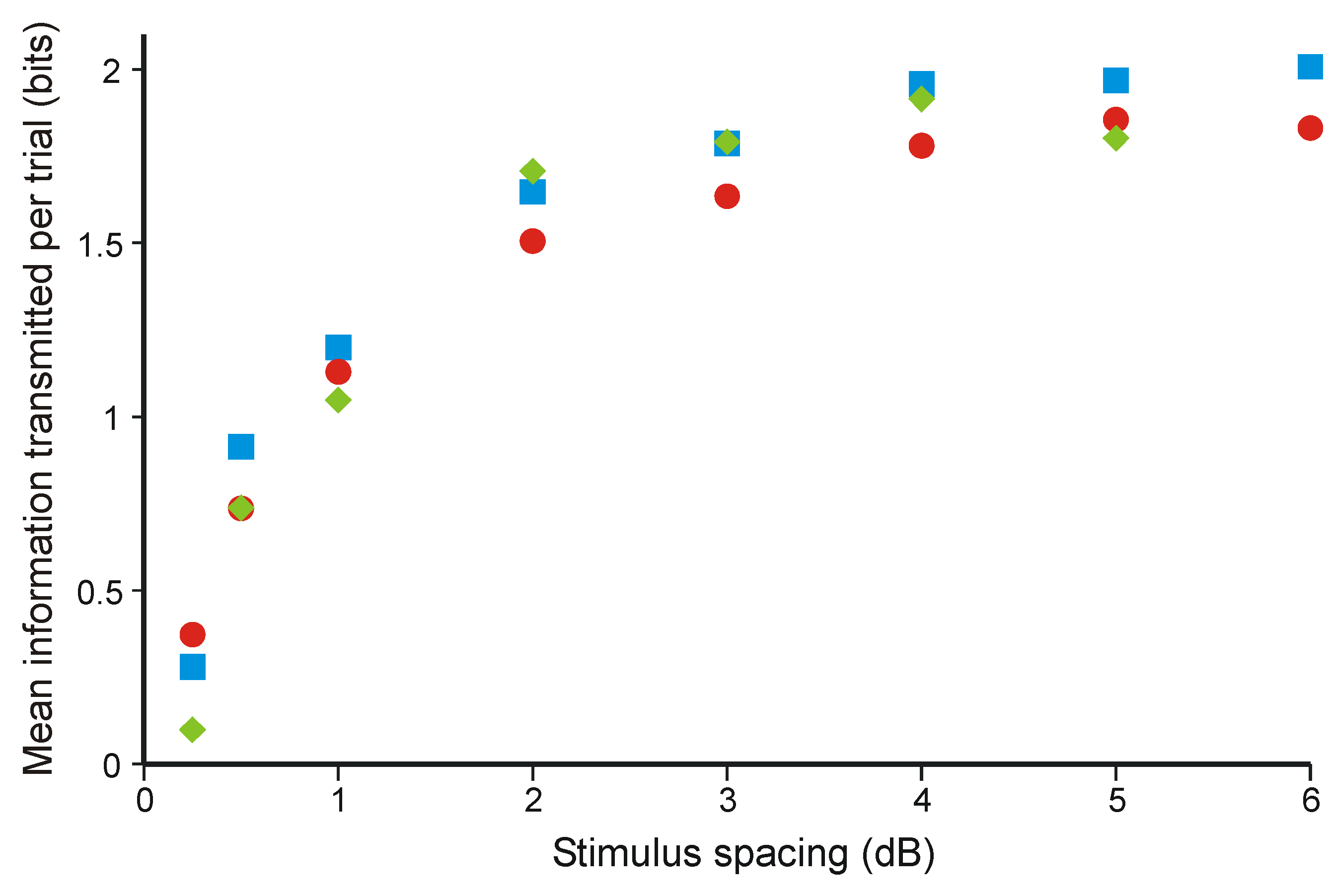
4.2. Combining Information from Different Sensory Modalities

The normal, equal variance, signal detection model routinely accommodates discriminations between two separate stimuli of magnitudes X and XX—two flashes of light in darkness, two bursts of noise in silence, two weights to be lifted in succession—in all sensory modalities e.g., [78,79,80,81,82]. In addition, the frequency of a correct response in the method of constant stimuli increases as a normal integral with respect to ΔX, at least for small values of ΔX (e.g., [79,83,84], [85]—data re-presented in [86,87]—[88,89]). It follows that d' increases in proportion to ΔX, and if ΔXθ is the value of ΔX affording 84% correct responses (equivalent to d' = 1), (ΔXθ)-2 is proportional to the divergence of the discrimination. Suppose now that a discrimination is presented simultaneously in two different sensory modalities (vision and touch below), with 84% thresholds ΔXθv and ΔXθt respectively. Then the divergence of the combined discrimination, simultaneous in both modalities, should be proportional to
Xθvt)-2 = (ΔXθv)-2+(ΔXθt)-2
Ernst and Banks [90] tested Equation 34 by presenting a size discrimination simultaneously by vision and by touch. Participants viewed a visual stimulus generated on a cathode ray tube and reflected in an opaque mirror, so positioned that the visual stimulus appeared to be at the same location in space as a tactile stimulus to be felt between finger and thumb; but participants were not, at the same time, able to see their hand grasping the tactile stimulus. The standard stimulus had a thickness of 55 mm, and was first judged by vision and by touch alone to estimate ΔXθv and ΔXθt separately. Then the stimulus was presented simultaneously to both senses to estimate ΔXθvt. The three threshold estimates conformed satisfactorily to Equation 34.
On some trials Ernst and Banks [90] presented the standard stimulus with different thicknesses X in the visual and tactile modalities, differing by ±1.5 mm or ±3 mm about a mean of 55 mm. this was designed as an additional test of the manner in which information from the two senses is combined. The 50% point on the psychometric (discriminability) function adjusts to match the perceived mean of the standard stimulus. Where the visual and tactile version of that standard were different, the estimated point of subjective equality was a weighted average of the separate standards, with weights approximately (ΔXθv)-2 and (ΔXθt)-2 respectively.

4.3. Weber’s Law

In addition to the shapes of the signal-detection operating characteristic and the discriminability function noted above, difference thresholds also conform to Weber’s Law down to about absolute threshold (e.g., [85,91,92], [93,94]—these last two sets of data re-presented in [95]). (The amplitude of a pure tone, but not Gaussian noise, and the contrast of a sinusoidal grating, are two known exceptions to Weber’s Law). All these results can be accurately modeled with a family of χ2 distributions of a common number of degrees of freedom, increasing in scale in proportion to X [86,87]. The point of interest here is the derivation of this model from a simple consideration of information throughput.
A visual stimulus at the physical level of description (to take the simplest case) is a Poisson stream of quanta of density proportional to the stimulus luminance, L. This stimulus needs to be modeled as a random process unfolding in time (and equally area). Each quantum absorbed is absorbed within some particular receptive field in the retina to produce a small perturbation in cellular potential extending over some small range of area and time. The sensory process can therefore be approximated, at this initial stage, by dividing the area and duration of the stimulus into small segments, δ(AT); the quantal absorptions are then (assumed to be) summed within each segment, while separate segments are processed independently.
Now consider a discrimination between two stimuli of luminances L1 and L2. The quantum catch within each segment has probability function
pr = eαr/r!
where α = L1δ(AT) or L2δ(AT) according to the stimulus presented. The probability ratio in favor of luminance L2 is
e - ( L 2 - L 1 ) δ ( A T )  ( L 2 / L 1 ) r
and the information in favor of L2 and against L1 in r quantal absorptions is
I(L2, L1; r) = – (L2L1)δ(AT) + r ln(L2/L1)
Aggregate quantum catch. Aggregating information over the entire area and duration of the stimulus gives
I(L2, L1; Σr) = – (L2L1)AT+ Σr ln(L2/L1)
so that the total number of quantal absorptions is a sufficient statistic for the discrimination. The divergence of this discrimination is
E{I(L2, L1; Σr)| L2} – E{I(L2, L1; Σr)| L1} = (L2L1)AT ln(L2/L1)
This is the quantity in this Poisson model analogous to d'2 above. Luminance L2 can therefore be distinguished from L1 with 75 per cent accuracy when
√[(L2-L1)AT ln(L2/L1)] = 1.349
twice the probable error in the normal model). Writing L for L1 and LL for L2, this relation becomes
√[AT ΔL ln(1+ ΔL/L)] ≅ √[AT ] ΔL/L = 1.349
If ΔL in Equation 41 be replaced for the moment by the small difference δL, this equation implies that the Poisson analogue to d' increases as δL; that is, the discriminability (psychometric) function is approximately a normal integral with respect to δL; this accords with observation. But the factor √L implies that threshold, ΔL, increases only as the square root of luminance, not as the luminance as Weber’s Law requires. A square root law is sometimes observed at low luminances [96,97,98—see also below], but if Equation 41 be extrapolated to high luminances, there must be an increasing loss of information in transmission to accord with observation.
This problem was first identified by Fullerton and Cattell [99], since when many psychologists have attempted to explain how that increasing loss of information comes about. Laming (see p. 71 [100]) lists five ideas that have recurred repeatedly in the literature. This problem cannot be resolved, however, solely on the basis of discriminations between separate stimuli. Laming [86,87] exhibits two distinct models, both of them representing all the data from discriminations between separate stimuli with superb accuracy, but based on quite different underlying principles of sensory analysis.
Comparison needs to be made with a discrimination between the same two luminances presented in different spatial or temporal configurations (see [101]). If experiments are chosen (e.g., [80,85]) in which the same stimuli, differing only in the configuration of the two luminances to be distinguished, are presented to the same eye of the same observer within the same experimental paradigm, then any difference in discriminative performance must be due to the interaction of the sensory analysis (the ‘coding’ which is assumed to be fixed) with the different configurations of the stimulus levels to be distinguished.
Compare the uniform stimulus of Equation 37 with a bipartite field of which half has luminance L1 and half L2. The different luminances are contiguous. A simple calculation based on Equation 38 says the threshold for discrimination should be raised two-fold (because luminance L2 now covers only half the field); but, in truth, the boundary between the two luminances can be detected at one-tenth the difference needed to distinguish two separate luminances (comparing [102] with [103]—see Figure 7.2 [100], or [104] with [105]). Even more compelling, the detectability (psychometric) function is approximately a normal integral with respect to (δL)2 [85]; that is, empirically, d' ∝ (δL)2 and divergence, substituting δL for (L2-L1) in Equation 39, ∝ (δL)4. If the logarithmic term in the divergence be expanded in more detail,
AT δL ln(1+ δL/L) = AT δLL/L ½(δL/L)2 + ⅓(δL/L)3 – …)
and, in the detection of spatial boundaries and temporal discontinuities, the terms in δL/L and (δL/L)2 in the expansion of ln(1+ δL/L) do not show.
Variance of the quantum catch. Suppose, now, that sensory discrimination is differentially coupled to the physical stimulus. The visual system is sensitive to boundaries and temporal changes, especially when they are sinusoidal in form. It is not sensitive at all to absolute luminance, and performs as though it were differentially coupled to the physical world. Other sensory modalities are similar. It is not meaningful to differentiate a Poisson process, and I use the term “differential coupling” (below) to denote the cancellation of the Poisson mean between the positive and negative components of each receptive field.
The input from each segment, δ(AT), of the stimulus field now consists, not of a single Poisson process, but of the difference of two independent such processes, both of density α = ½Lδ(AT); that is, the previous input of density Lδ(AT) is now divided into two components, one positive and one negative. Since the Poisson distribution tends to the normal as α increases, the aggregate input approximates a Gaussian noise process of power 2α, or Lδ(AT), and aggregation over the entire field gives a total power of LAT, the product of luminance, area and duration of the stimulus. The energy in a sample of Gaussian noise is distributed (approximately) as χ2 with some number of degrees of freedom ν, multiplied by the power divided by ν, so that the mean is equal to the power. Increasing the power from L1AT to L2AT simply increases the scale of the distribution by L2/L1 and a simple geometric argument says that L2 can be distinguished from L1 when L2/L1≥ some constant; this is Weber’s Law. The logarithm of a χ2 variable is approximately normal, so that the discriminability function is approximately a normal integral with respect to ln(L2/L1), which gives a slightly better representation, better than a normal integral with respect to δL, of what is observed [86,87].
The idea that sensory discrimination is differentially coupled to the physical stimulus admits a simple realization at an elementary level in the sensory pathway. Sensory neurons admit both excitatory (positive) and inhibitory (negative) inputs. The two are balanced and a static uniform input leads rapidly to the decay of any neural response, as every electro-physiologist discovers; except that the positive-going excursions of the Gaussian noise are transmitted as a maintained discharge. However, the positive and negative components of the receptive field do not match exactly, so that temporal changes in input elicit a brief transitory response (e.g., [106]). Envisage that the eye is moving (micro-saccades) with respect to the physical stimulus. (If the stimulus is stabilized on the retina, perception fades within a very few seconds; [107,108]). As a receptive field unit traverses the boundary of the bipartite field, there is an increment or a decrement (depending on the direction of traverse) in input, so that units in the neighbourhood of the boundary receive an additional variability in their input proportional to (δL)2. (It is essential, of course, that the two luminances of the bipartite field are contiguous, essential both to this argument and to the different empirical properties of the discrimination). The aggregate variability of the input to the sensory pathway is increased when the boundary is present. It is now distributed as a non-central χ2 with non-centrality proportional to (δL)2. this at once provides a more sensitive detection of boundaries and temporal discontinuities than a simple comparison between different luminances, but the detectability function now increases as a normal integral with respect to (δL)2, not δL or ln(L2/L1) (see [100,109]).

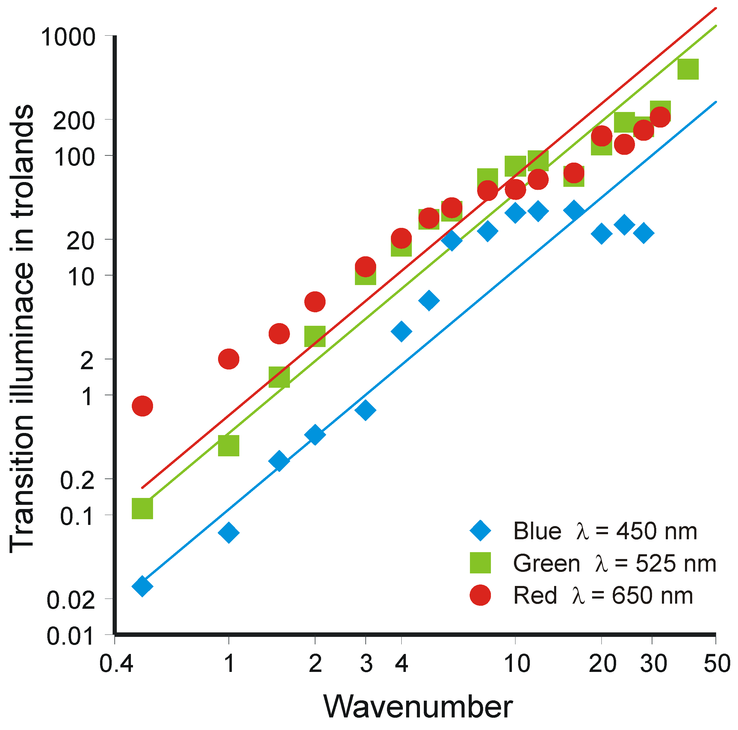
4.4. Parallel Channels in Vision

One of the explanations previously proposed for Weber’s Law suggested that retinal adaptation scaled stimulus luminance down in strictly inverse proportion, so that physical luminances L and L+ ΔL become, internally, 1 and 1 + ΔL/L (e.g., [110,111]). Discrimination can then depend only on ΔL/L. A scaling down of this nature does indeed occur in the retina, but does not give Weber’s Law [112]. Instead, it leads to an improvement in visual acuity as luminance increases and, more important, enables vision to function over a range of luminance much greater than the dynamic range of any one neural unit. The contrast thresholds from van Nes [113] in Figure 4 show how this comes about.
The stimulus in Figure 4 was a static field, 8.25° and 4.5° wide, observed in Maxwellian view through an artificial pupil of 2 mm diameter. Luminance was varied in a horizontal direction according to Equation 19 above. Upper (grating just visible) and lower (grating just not visible) thresholds were determined by the method of limits, and the values plotted in Figure 4 are the geometric means of each pair of thresholds. Threshold decreases approximately as a square root law (gradient –½ with respect to the double logarithmic co-ordinates) up to a transition illuminance, Ltrans, and thereafter remains approximately constant. To emphasize this relation, the thresholds for each wavenumber have been fit with a rectilinear characteristic. The estimates of Ltrans, both for the data in Figure 4 and for two other sets of threshold measurements with red (λ = 605 nm) and blue (λ = 450 nm) light are shown in Figure 5, where they are each compared with the best-fitting straight line of gradient 2, corresponding to the relation
Ltransg2
Since these thresholds are limiting values for the proportionate variation in luminance that can be detected, a constant value corresponds to Weber’s Law and gradient –½ corresponds to an increment threshold increasing as the square root of illuminance. The argument that follows uses the fact that the same distribution of stimulus information, subject only to a difference in luminance, issues in one distribution of output information below Ltrans and a different distribution above. This leads to some inferences about the organization of the visual pathway.
Figure 4. Contrast thresholds from van Nes [113]. The rectilinear characteristic fitted to each set of thresholds represents a square root law at low illuminances and Weber’s Law at high ones.
Entropy 12 00720 g004
Sensory discrimination differentially coupled to the physical stimulus within each receptive field requires quantal absorptions in the negative input to be opposed to absorptions in the positive input. If the Poisson density is sufficient, so that successive absorptions overlap, this condition is satisfied; the mean inputs will certainly cancel. But at a low enough luminance the quantal absorptions will only occur one at a time, one in the positive input, now one in the negative (see [114]). In this case the negative inputs have no corresponding positive input to cancel—they are of no effect—and the positive inputs are transmitted uncancelled.
The transition illuminance marks a boundary between values of luminance at which the positive input to the receptive field is transmitted ‘as is’ and higher values at which the mean positive and negative inputs cancel. It is the illuminance at which the two inputs become sufficiently dense for cancellation to take effect and represents the same level of input in each receptive field. (In practice, the transition from square-root to Weber Law behavior is gradual, not instantaneous as represented by the rectilinear characteristics in Figure 4). While that level of aggregate input increases in strict proportion with illuminance, it is also proportionate to the area of the receptive field. Since the transition illuminance is different for different wavenumbers, it follows the each wavenumber is preferentially detected by a different neural unit. In each case in Figure 5 the transition illuminances increase approximately as the square of the wavenumber. Now, if it be supposed that the receptive fields sensitive to horizontal modulation of luminance are generally of the same shape, but of different sizes (in linear scale), then wavenumber g will be preferentially detected by a field of scale proportional to g-1 and therefore of area g-2. The net input to such a field from a physical illuminance L will be proportional to Lg-2, and if that input is just sufficient to produce Weber law, rather than square root law, behavior, Ltransg-2 = constant, which is Equation 43.
Figure 5. Transition illuminances estimated from the data of van Nes [113]. (From Sensory Analysis, by D. Laming, p. 204. London: Academic Press, 1986. © Copyright Elsevier 1986. Reproduced by permission.).
Entropy 12 00720 g005
Physiological investigation is needed, of course, to tell us which neurons are the ones that detect sinusoidal modulations of luminance. For example, Legge [115] has demonstrated differences between monocular and dichoptic masking of gratings that show the initial units sensitive to sinusoidal modulations of luminance to be monocular. Campbell and Kuikowski [116] had previously shown that monocular masking of one grating by another was both wavenumber and orientation specific. So Hubel and Wiesel’s [117] identification of simple cells in layer IVb of the striate cortex as predominantly monocular, but sensitive to both wavenumber and orientation, seems to match the psychophysical findings. Since the quantum catch is determined in the retina, the evidence suggests that neurons in the visual cortex sensitive to a specific wavenumber take their inputs from receptive fields of proportionate size in the retina and this leads to the notion of parallel channels in the visual pathway [34].
It might be supposed that physiological investigation is all that is needed and that analysis of the information transmitted in sensory discrimination (and other tasks) tells us nothing new. This would be a mistake. Physiological investigation can tell us which neurons respond to which stimulus attributes and which other neurons they receive inputs from. But the functional relationship of neural activity to sensory input and thereby to perception and the functional relationship between neurons can be discovered only by modeling the information transmitted. There is an obvious problem in that perceptual experiments are carried out on human participants and electrophysiological recordings are from cats and monkeys. There is also another, less obvious, problem in that the electro-physiologist records the response of a single neuron to whatever (single) stimuli are of interest, while the experimental psychologist must, of necessity, present each stimulus to the entire visual pathway. Because that pathway is functionally a set of parallel channels and all channels are engaged by each stimulus, the wavenumber-sensitivity of any one channel can be discovered only from the detectability of compound gratings (e.g., [118]) or from the masking of one grating by another (e.g., [116]). The interpretation of such threshold measurements depends on how the separate sinusoidal components are thought to interact (see pp. 99–102 [34] for alternative proposals), and only then can comparisons be made with single-unit recordings (e.g., [119,120]). In the case of simple cells the problem is unusually acute since bandwidths appear to vary widely [121]. To put the problem succinctly, a functional map of the pathway (e.g., [114]) needs to come first; only then can neurophysiological findings be meaningfully fitted in.

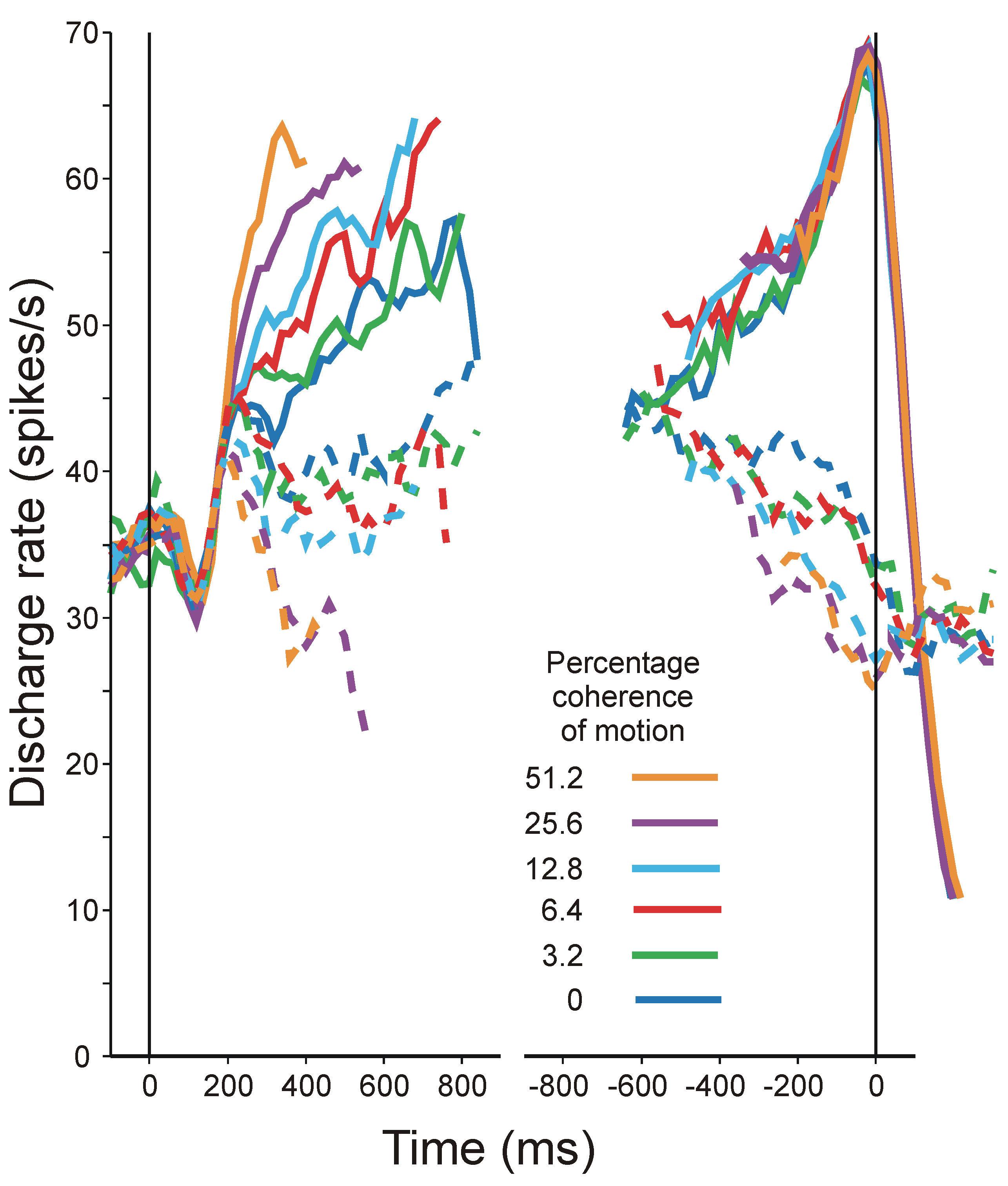
4.5. Accumulation of Information in the Brain

Roitman and Shadlen [122,123] report this experiment: Two rhesus monkeys viewed a circular field, 5° diameter, within which were a number of randomly placed dots. Some proportion of those dots moved coherently, either to the left or to the right. The monkeys were trained to move their eyes in the direction of motion to orient one of two targets placed one each side of the stimulus field. As the monkeys performed this task, the activity of a neuron in the lateral intra-parietal area (LIP) of the inferior parietal lobe was recorded. The neuron was selected to have a response field that covered one of the two targets, while the other target was located well outside. The discrimination task therefore initiated an eye-movement either into, or well away from, the response field of the neuron. The discrimination task was presented in two different forms. In one a delay was interposed between the termination of the stimulus (duration 1 s) and the monkey’s response. This was accomplished by having the monkey wait (0.5 to 1.5 s) until a fixation point disappeared. The neuron was also chosen such that it emitted sustained output during this delay period. In the other form the monkey was trained to respond as soon as the direction of motion could be determined. In both forms of the task errors were signaled by a short time out (750 ms).
Figure 6 presents some averaged discharge frequencies (spikes/s) from this experiment. The difficulty of the discrimination could be manipulated by varying the proportion of the random dots that were made to move coherently; different traces in Figure 6 represent averaged data for 51.2, 25.6, 12.8, 6.4, 3.2 and 0% coherence. Different trials required the monkey to orient viewing into, or away from, the response field of the neuron. Discharge rates followed by eye-movements into the response field are shown by solid lines, away from the field by broken lines. Each trial is terminated after a variable duration by a saccade. The discharge rates from different trials have been averaged in two different ways: The left-hand half of the diagram shows the averaged firing rates when the records from different trials are aligned with respect to the onset of the motion stimulus (at 0 s), but excluding responses within 100 ms of the saccade; the right-hand half shows the same population of recordings aligned with respect to the saccade (at the new 0 s), but now excluding responses within 200 ms of stimulus onset.
On the right-hand side of Figure 6 a saccade begins when the discharge rate reaches about 68 spikes/s; this average is independent of the coherence of motion in the stimulus, and hence of the difficulty of the task. But task difficulty does impact on the rate of increase in average firing rate on the left-hand side of the figure; the lower the coherence of motion, the slower is the build-up to 68 spikes/s. When motion is directed in the opposite direction, away from the response field of the neuron, discharge rate decreases. That decrease is faster when the discrimination is easier; it mirrors the faster increase observed with easier discriminations when the eyes orient into the response field of the neuron.
Likewise, at the initiation of the saccade (in the opposite direction) the discharge rate has fallen to an average of about 26 spikes/s. The neurons from which these recordings were made do not themselves initiate that eye-movement away from their response field; it is a very strong presumption that there is some other neuron in LIP, not under the recording electrode, driving the eyes in the opposite direction. These results suggest, strongly, that the increasing rate of discharge represents an accumulation of input relevant to the direction in which an eye-movement will be required. Roitman and Shadlen [122] propose that the activity of LIP neurons represents the temporal accumulation of direction-selective sensory evidence, obtained by integrating the output of neurons in the middle temporal regions that are known to be sensitive to direction and strength of motion [124,125]. When movement is required in the opposite direction, the rate of discharge decreases (which is why it was important to choose neurons with a sustained response during the delay period). The combination of averaged discharge rates that increase or decrease according to the direction of the saccade that follows, with random fluctuations within those averaged rates, suggests a random walk as a statistical model for this process. Of course, the neuron under the microelectrode might not be the only one with a response field covering the target; a more realistic model would envisage a population of neurons in LIP that modulate their discharge rates according, in this case, to stimulus input and jointly determine the direction of the subsequent saccade.
Figure 6. Averaged neural responses from 54 LIP neurons in the reaction-time task of Roitman and Shadlen [122]. On the left hand side averaged responses are aligned with respect to stimulus onset and exclude all perisaccadic responses (within 100 ms of saccade). On then right hand side averaged responses are aligned with respect to the initiation of the saccade and exclude all responses within 200 ms of stimulus onset. Solid lines indicate neural responses leading up to a saccade towards the response field of the LIP neuron; broken lines indicate neural responses leading to a saccade away from the response field. Data for correct responses only from Roitman and Shadlen [122]. (Adapted with permission of Society for Neuroscience, from The Journal of Neuroscience, Volume 22, p. 9482. © 2002 Society for Neuroscience; permission conveyed through Copyright Clearance Center, Inc.).
Entropy 12 00720 g006
Whether the increasing discharge rate in Figure 6 can truly be interpreted as the evolution of the monkey’s decision in favor of one direction rather than the other, after the manner of the sequential probability ratio test model for two-choice-reaction times (see pp. 39–40 below, [42], [126]) depends on what happens on trials on which the monkey makes an incorrect response. All the records in Figure 6 were taken from trials on which the monkey oriented vision in the direction indicated by the stimulus. However, Roitman and Shadlen (see Figure 11 [122]) also make comparison between correct and error trials at motion coherences of 3.2 and 6.4%. There are some differences consequent on the fact that these are difficult discriminations (necessarily so to provide enough data for the comparison). Threshold (82% correct) was estimated at 6.3% motion coherence, so these discriminations are at or below threshold. Often there will be insufficient information in the stimulus presentation to determine the direction of motion; in consequence, at these levels of difficulty, errors tend to take longer than correct responses. Nevertheless, on an error trial the trend of activity in LIP neurons matches the direction of the subsequent saccade, not the direction of motion. There is, therefore, a prima facie case that the traces in Figure 6 represent a neural accumulation of evidence in favor of an eye-movement towards (or away from) the response field of the neuron, analogous to the build-up of information in a sequential probability ratio test.
This is to look at the discrimination of direction of movement from the point of view of the monkey—should I look left or right?—or of a statistician conducting a sequential probability ratio test. But there is another way of looking at the matter. If the experimental set-up and the monkey be jointly considered as a single physical system, a different view emerges, not necessarily alternative. The control of output (in this case, eye-movement) has to be under integrative control because the sensory input is differential. Differential coupling has been demonstrated above with respect to luminance, but is equally true of motion, which has the perceptual properties of a primary stimulus attribute, notwithstanding that motion is itself differential with respect to spatial location (see Chapter 4 [73]). The random component of the integration arises, of course, because the sensory input is partially random, and random walk control of output is only to be expected. This argument applies generally to the control of all kinds of motor output; the experiment by Roitman and Shadlen [122] is simply the clearest demonstration to date.

4.6. Interim Conclusions

Sending a message through a communication system is, as I have already pointed out, an experiment. At the same time, an experimental trial—a stimulus is presented and the participant makes a response—is the sending of a message through a communication system. The human subject can be viewed as a communication system with fixed ‘coding’. There is no capacity limitation; instead we need to discover what ‘coding’ is fixed in the system. That is not too difficult. The signal-detection operating characteristic gives a direct estimate of the distribution of information implicit in the participant’s decision and that distribution can be compared with a similar distribution of the information supplied by the stimulus. A purely functional, information-theoretic description of the human operator can be developed in this way. This is roughly what cognitive psychologists have been attempting for four decades past. What information theory offers is a quantitative platform to support investigations of greater reliability. There is no need to understand how the system works at the physical level of description, in terms of individual neural responses. An information theory will actually be simpler to construct and will provide a guide to a subsequent fuller, neural-level, description.

5. Bayes’ Theorem

Signal-detection performance is demonstrably affected by the relative frequencies of signal and noise, and two-choice reaction times are similarly sensitive to stimulus probabilities. The question therefore arises how prior probabilities interact with the information revealed by the signal-detection operating characteristic. The optimum manner of combining information from two different sources is prescribed by Bayes’ theorem (Equation 24), which specifies how posterior probabilities may be calculated from the combination of prior probabilities and a probability ratio derived from experimental data. But prior probabilities cannot interact with human performance directly because they are merely abstract parameters of the experimental design. They can interact only through the actual presentation of stimuli.
Although human performance is manifestly influenced by the relative frequencies of different stimuli, that influence is often less than optimum. For this reason it has long seemed an attractive idea to invoke subjective probabilities, different from the objective ones, to account for otherwise inexplicable behavior, and then infer what those probabilities have to be from observation of the behavior itself. Oaksford and Chater’s [52,53] treatment of Wason’s selection task is a case in point. But this procedure does not explain the behavior because the prior probabilities thereby introduced are not equated with any independent variable of the experimental design. In fact, it does no more than introduce additional free parameters, and can hardly be said to be a legitimate invocation of Bayes’ theorem. Moreover, if rigorous questions be asked about the consistency of the subjective probabilities, the resultant problems are sufficient to make the idea fall apart [127].
In what follows I confine attention to the relationship between independent prior probabilities, that is, between parameters of the experimental design, and human performance. In each experiment the stimulus presentation probabilities are nominally fixed within each block of trials, but are different in different blocks. The question at issue is whether the effects of the relative frequencies of different stimuli in those different blocks may be accurately described by Equation 24. If the presentation probabilities were to be changed without notice to the participant, then Bayes’ theorem would thereafter deliver the wrong prescription, and one might view the results surveyed below as a reflection of the manner in which people adapt to potentially changing contingencies. Unannounced manipulations of stimulus probabilities, however, do not feature in the experiments below.

5.1. Two-Choice Reaction Experiments

There are two alternative signals. In the experiment referenced below the stimuli were vertical white stripes on a black ground, 0.5 in wide and respectively 4 and 2.83 in tall, exposed in a multiple Dodge tachistoscope. One of two responses (keys pressed with the left and right forefingers) is to be made “as quickly as possible”. The reaction time varies substantially from trial to trial and one interesting idea is that latency is determined by the time taken to collect sufficient information to make a response to some desired level of accuracy. (But the information is now information in favor of one signal and against the other, so that this idea is quite distinct from optimal transmission through an ideal communication channel). Imagine that the experiment of Equation 1 is repeated many times and the data accumulated until there is sufficient to prove one hypothesis or the other. if i indexes successive replications, then, adapting Equations 2 and 24,
ln [ P ( H 1 | i X i ) / P ( H 0 | i X i ) ] = ln [ P ( H 1 ) / P ( H 0 ) ] + i ln [ P ( X i | H 1 ) / P ( X i | H 0 ) ]
The sequence of replications {Xi} continues until the posterior information (on the left of Equation 44) reaches some desired value, a value that guarantees that Response 1 (H1), rather than Response 0 (H0), is correct to within some small degree of error. Expressing this formally, the sequence of replications {Xi} continues so long as
ln ( ε 0 / ( 1 ε 0 ) ) < ln [ P ( H 1 ) / P ( H 0 ) ] + i ln [ P ( X i | H 1 ) / P ( X i | H 0 ) ] < ln ( ( 1 ε 1 ) / ε 1 )
where ε0 is the probability of error when R0 is selected and ε1 likewise the probability of error conditional on the selection of R1. These are probabilities of error conditional on the response and need to be distinguished from the probabilities of error conditional on the stimulus, which are
α = P ( H 1 ) / P ( H 0 ) ε 0 / ( 1 ε 0 ) ( 1 ε 1 ) / ε 1 ε 0 / ( 1 ε 0 ) β = P ( H 0 ) / P ( H 1 ) ε 1 / ( 1 ε 1 ) ( 1 ε 0 ) / ε 0 ε 1 / ( 1 ε 1 ) }
here α is the significance level of the test (the probability of error conditional on H0) and 1-β is its power. The participant chooses a desired level of accuracy and the reaction times follow stochastically from Equation 45. The mathematics required to develop this idea is the sequential probability ratio test [128], and the application to reaction times was first suggested by Stone [126]. In effect, Bayes’ theorem is continuously and repeatedly applied to test the validity of the evidence.
The data from Laming (Experiments 1 & 2 [42]) raises two issues. These two experiments compared five different presentation series in which the proportions of the two signals, randomly ordered, were, respectively, 0.25:0.75, 0.37:0.625, 0.5:0.5, 0.625:0.375, and 0.75:0.25. Two-choice reaction performance is exquisitely sensitive to the relative frequencies of the two signals. The more frequent signal receives the faster response and gives rise to fewer errors absolutely, notwithstanding the increased number of trials on which that particular error might occur. This in itself points to the sequential probability ratio test as a possible model. The first question (the second follows later) asks whether the different numbers of errors in these different presentation series can be explained directly by the different prior probabilities, that is, whether Bayes’ Theorem adequately accounts for the variation in numbers of errors according to Equations 46.
If the choice process (Equation 44) is symmetric between the two signals, then it is optimum to set ε1 equal to ε0, so that each response is made to the same small degree of posterior error (Theorem A.3, p. 128, [42]). However, the decision process in these experiments is slightly asymmetric (see Figure 10 below), so that the more general formulae in Equations 46 must be used. The criteria ε0 and ε1 can be estimated from the proportion of decisions in favor of H0 (H1) that are incorrect, and insertion in the formulae of Equations 46 gives the results, observed proportions and model predictions in Figure 7.
Figure 7. Error scores and model predictions from Laming (Experiments 1 & 2 [42]).
Entropy 12 00720 g007
The comparison between model and outturn is significant for Experiment 1 (χ2 = 69.811, with 8 d.f., p. < 0.001), but not for Experiment 2. The difference is instructive. The participants had to experience the five series in some order and in Experiment 1 a demonstrable ‘carry-over’ effect was discovered from the relative frequencies in one series to performance in the next. That is to say, the distribution of errors in a given series was dependent, not just on the relative proportions of the signals, but also on the relative proportions in the previous series. Experiment 2 was redesigned in an express attempt to balance this (by then known) factor. The different series were presented with the probability of Stimulus 0 in strictly increasing/decreasing order, each to half of the participants. Comparison of the numbers of errors shows that the two orders of presentation produced different results (χ2 = 63.979, with 16 d.f., p. = 0.000). The constituent conditions are presented separately in Figure 7b, and the ‘carry-over’ effect can be seen in the systematic differences of both error scores and model predictions between the two orders of administration. The model statistics are: P( Stimulus 0 increasing), χ2 = 19.038, with 8 d.f., p. = 0.015; P (Stimulus 0 decreasing), χ2 = 12.694, with 8 d.f., p. = 0.123.
While the numbers of errors do show a striking variation with stimulus probability of a pattern that is approximately captured by Bayes’ Theorem in combination with the sequential probability ratio test, there are other factors that also affect the issue. Stimulus probabilities were realized in these experiments by the presentation of a random sequence of stimuli with the required statistical properties, and the hypothesis must be considered that participants adjust to those statistical properties, not by a calculation based on Bayes’ Theorem, but by pragmatic trial-to-trial adjustments, depending on the stimulus presented and the response made on each trial (see esp. Chapter 8 [42]). The ‘carry-over’ effect described above is a part of this adjustment. A re-examination of some signal-detection data reinforces this idea.

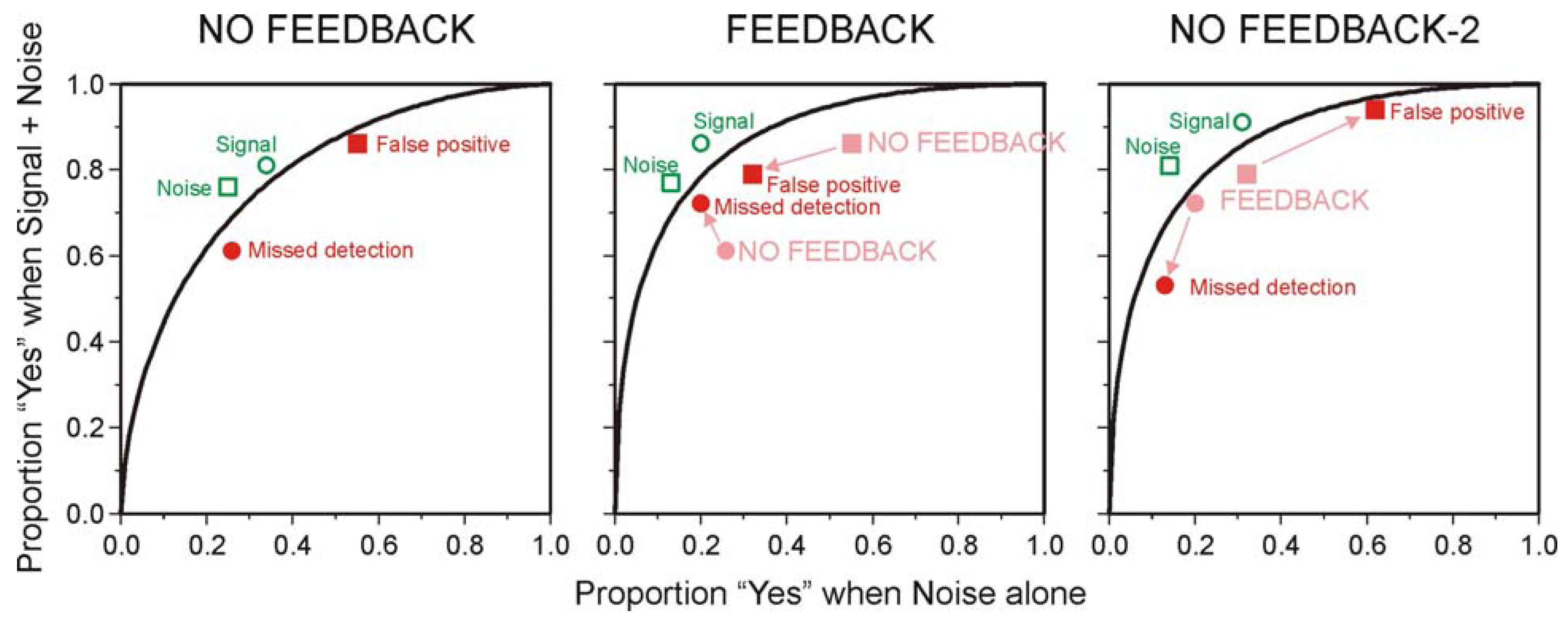
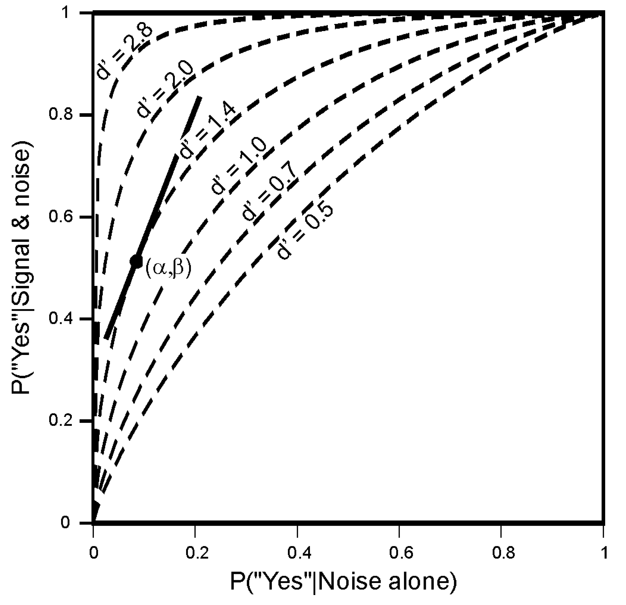
5.2. The Choice of Criterion in Signal Detection Experiments

If signal detection data accord accurately with a normal, equal variance, model, there is a particular location of the criterion, varying with signal probability, that minimizes the total number of errors [19]. Figure 8 (Observer 1) compares two sets of calculations, one labeled ‘Bayes’ theorem’ from Green and Swets (see p. 90 [16]) and another labeled ‘Probability matching’ based on a suggestion by Thomas and Legge [129]. The abscissa is the probability of signal-plus-noise (with the 0.3 and 0.7 values relocated slightly so that the calculations based on ‘Bayes’ theorem’ are exactly collinear) and the ordinate (log scale) is the likelihood ratio attaching to the operating point (cf. Figure 1), either observed or calculated. Both these calculations use data from one observer in the experiment by Tanner, Swets, and Green (see Figure 4-1 [16], [130]). Figure 8 (Observer 2) presents an equivalent set of calculations from the other participant in the experiment by Tanner, Swets, and Green [130]. The data from this second participant are highly asymmetric (see Figure 4-5 [16]) and have been modeled here with a χ2/non-central χ2 model (pp. 256–259 [100]), which gives different results in the calculation for ‘probability matching’. In both cases, ‘Probability matching’ accords reasonably accurately with observation, while the calculations based on ‘Bayes’ theorem’ do not.
The optimum calculated from Bayes’ theorem (red squares) would minimize the total number of errors, and it can readily be seen that the actual likelihood ratio at the estimated criterion (open diamonds) is always conservative, too close to unity, relative to this prediction. But suppose that, instead of minimizing the number of errors, the subject merely adjusts the frequency of “Yes” responses to match the frequency of signals—‘probability matching’. The concordance between the diamonds and the filled circles shows that idea to work well. But why?
In this experiment [130] the observer was given feedback on every trial and so knew immediately when he had made an error. Under such circumstances, observers will effect a large shift in criterion following an error, shifting in the direction that reduces the likelihood of a similar error in future (but increasing the likelihood of an error of the opposite kind). This was demonstrated by Tanner, Rauk, and Atkinson [131].
Tanner, Rauk, and Atkinson presented their subjects with a 100 ms 1 kHz tone at either 70 dB or at some lesser level adjusted to permit about 70 per cent correct responses. The proportions of 70 dB tones in different blocks of trials were 0.2, 0.5, and 0.8. There was no background noise. Figure 9, in which, for convenience of notation, the 70 dB tone has been designated ‘signal’ and the lesser level of tone ‘noise’, shows the aggregate performance of seven observers in the 0.5 condition. In this figure the data have been disaggregated according to the combination of events on the immediately preceding trial (distinguishing trials following correct responses to signal and to noise, false positives and missed detections, where ‘signal’ means the 70 dB tone).
The left-hand diagram presents the results from an initial total of 9,800 trials (1400 by each of 7 observers) in which the observers received no feedback. It can immediately be seen that performance (probabilities of a false-positive and of a detection) is related to the combination of events on the preceding trial. The picture is consistent with a criterion that fluctuates, though only slowly with respect to the succession of trials, with errors occurring chiefly at extreme deviations of the criterion.
Figure 8. Calculations of likelihood ratio at optimal criterion (‘Bayes’ theorem’) (From Green and Swets (p. 90 [16]), and of likelihood ratio given probability matching [129] using data from one observer in the experiment by Tanner, Swets, and Green [130].)
Entropy 12 00720 g008
The centre diagram in Figure 9 presents the next 9,800 trials in which the observers received the usual knowledge of results (as in the experiment in Figure 8). There is an overall improvement in discrimination, and performance following an error (of either kind) has shifted towards the centre of the operating characteristic. This is emphasized by copying the performance points following an error from the left-hand diagram. The knowledge that one has just made a mistake shifts the criterion for the next trial in such a way as to make a repetition of that particular mistake less likely; but that change simultaneously increases the likelihood of the alternative kind of error.
Figure 9. Performance following each kind of error and correct response in the 0.5-frequency condition of the experiment by Tanner, Rauk, and Atkinson [131]. (From Human Judgment: The Eye of the Beholder, by D. Laming, p. 179. London: Thomson Learning, 2004. © Thomson Learning, 2004. Adapted by permission.)
Entropy 12 00720 g009
This effect of knowledge of results appears again in the right-hand diagram in Figure 9, which summarizes performance from a further 24,500 trials without feedback. The improvement in discrimination (due to practice) is maintained, but the absence of feedback means that performance following an error, of either kind, is again at an extreme deviation of the criterion. The clear implication is that the signal-detection criterion does not have a fixed value, but evolves from trial to trial in a dynamic equilibrium. It is driven by large readjustments following each known error, and when feedback is supplied (Figure 8) will oscillate around a location where the absolute numbers of errors of each kind are equal. That equality means that the numbers of “Yes” responses lost through a mistaken “No” will equate approximately to the number gained through a mistaken “Yes”, and overall the frequency of “Yes” will match the frequency of the signals, as Thomas and Legge [129] suggested.
Table 6 sets out the absolute probabilities of error from Tanner, Rauk, and Atkinson [131], that is, the joint probabilities of ‘signal’ + ‘No’ and of ‘noise’ + ‘Yes’. For the feedback condition these absolute probabilities of each kind are approximately the same; but without feedback they differ widely, showing that it is the provision of feedback that equates the frequencies of errors.
The conclusion from these data is that in an experiment where one might, and many people did, expect prior probabilities to enter into a rational calculation based on Bayes’ theorem, that does not happen. Instead, performance is driven by successive shifts of the criterion, and large shifts too (see Figure 9), and oscillates around a dynamic equilibrium where the numbers of errors of each sort are approximately equal. A similar shift in criteria is apparent in two-choice reaction experiments, except that errors are few and the convergence to equilibrium is rarely complete. Following an error, the probability of a further error, of either kind, is depressed for several trials thereafter, and this reduction of error probability is accompanied by an increased reaction time. These effects are more noticeable with the response that was made in error; that is, the subject is particularly cautious when making that same response again [132]. The algorithm prescribed by Bayes’ theorem does not account for the observed effect of prior probabilities on the relative frequencies of the different kinds of error, not, at least, in signal-detection and two-choice reaction experiments.
Table 6. Absolute probabilities of error in the experiment by Tanner, Rauk, and Atkinson [131].
Probability of 70 dB tone
0.20.50.8
NO FEEDBACK
False positive0.3760.170.044
Missed detection0.0380.110.28
FEEDBACK
False positive0.0480.090.062
Missed detection0.0760.10.056
NO FEEDBACK-2
False positive0.2480.140.042
Missed detection0.0260.0750.152

5.3. Two-Choice Reaction Experiments (Again)

The second issue arising from choice-reaction data concerns the aggregation of information (Equation 44) during a single trial. The sequential probability ratio test is isomorphic to a random walk and can also be modeled as a diffusion process in continuous time. Notwithstanding the minor difficulties in modeling the errors (Figure 7 above), might that idea nevertheless be applicable to the human operator?
Figure 10 plots the mean reaction times for each signal in the same two experiments ( Experiments 1 & 2 [42]) against the information throughput. Setting aside questions about the optimum placement of response criteria, is reaction time linearly related to the information needed to make the response to whatever accuracy happens to be achieved? Estimating the functional relationship between mean reaction time and information throughput in Figure 10 presents a problem inasmuch as both variables are subject to random error. In consequence, neither the regression of mean reaction time on information throughput, nor that of information throughput on mean reaction time, is unbiased. However, it is certain that the functional relationship lies between these two extremes [133], and the pairs of regression lines in Figure 10 delimit that relationship sufficiently closely for the argument that follows.
The analysis in Figure 10 presupposes
Mean RT = Simple RT +
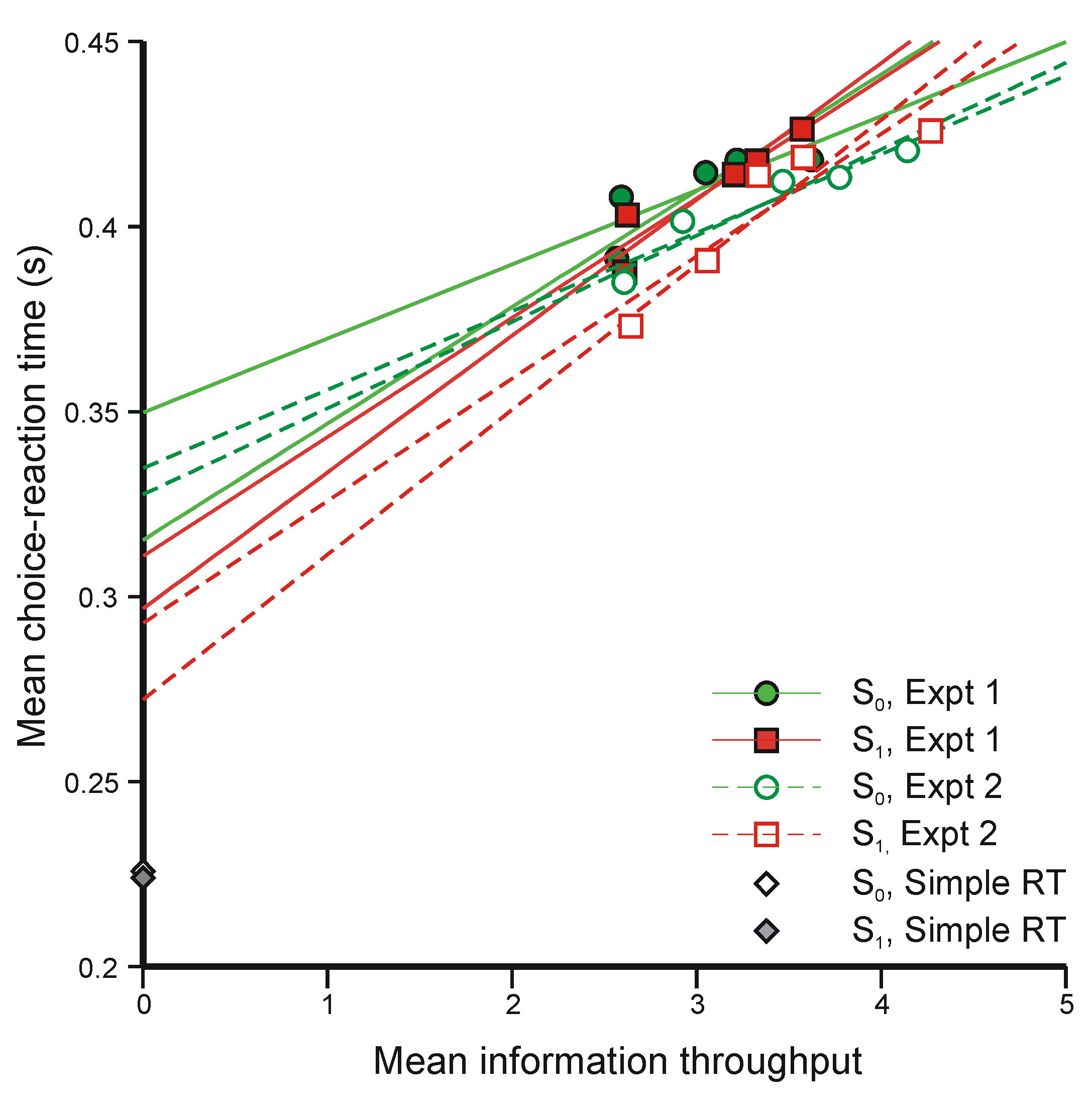
{Mean information throughput}/{Mean rate of transmission}
it being understood that ‘information transmitted’ is measured in the same manner as in Equation 44. The fact that the regression lines for the two different signals have different gradients (different mean rates of transmission) is not a problem; it is easy to construct statistical models with this property (see App. A in [42]). But there are nevertheless two reasons why Equation 47 will not do.
(i)
The regression lines in Figure 10 intersect at a positive value of information, whereas Equation 47 requires intersection at zero information. The model would still be tenable if the regression lines intersected at negative values of information, because ‘Mean information throughput’ is estimated from aggregate data. Since it is a non-linear function of that data, information could be lost in the aggregation. But intersection at positive values cannot be accommodated.
(ii)
Extrapolation of the regression lines to zero information gives an intercept very much greater than the measured simple reaction time for the same stimuli (about 0.22 s), represented by the diamonds on the ordinate (from Experiment 4 [42]).
To show why Equation 47 fails, I turn to an experiment on absolute identification.
Figure 10. Mean choice-reaction times from Laming (Experiments 1 & 2 [42]) plotted against mean information throughput. Two regression lines are shown for each set of data; these are the regression of mean reaction time on information throughput and information throughput on mean reaction time.
Entropy 12 00720 g010

5.4. Absolute Identification

The experiment (Experiment 4 [21]) has already been described in connection with ‘Information transmission in category judgments’ above. Figure 11 plots estimates of the variability of the identifications calculated in this manner. The presentation of each stimulus is represented by a random sample from a normal distribution. The normal distributions all have the same variance (σ2; i.e. Torgerson’s [135] Law of Categorical Judgment, Class 1C), and the means are set equal to the decibel values of the respective stimuli. This leaves the variance, σ2 (in units of dB2), as the only free parameter, chosen to best fit the data. Figure 11 plots the best-fitting values of the variance, separately estimated for three individual subjects, against (the square of) the spacing of the stimuli. the estimated variances increase approximately linearly with the square of the dB spacing, with a small intercept, 1.52 dB2.
The important feature of these data is that, except for the declining influence of the small intercept (which is arguably the variability contributed by the sensory process), resolution does not improve with a wider spacing of the stimulus values (cf. Figure 3). Instead, the (linear) magnitude of errors of identification increases in proportion to the stimulus spacing. That is, the accuracy of identification of the stimuli is tied to the spacing of the geometric ladder of stimulus magnitudes used in the experiment and is equivalent to a purely ordinal scheme of identification (see Chapter 10 [136]). Putting this another way, the judgment of one stimulus relative to another (or, indeed, relative to an internal standard if one exists) is no better than < greater, about the same, less >. the aggregation of such crude ordinal comparisons cannot support a sequential probability ratio test procedure of the kind envisaged in Equation 47—that is the point I emphasize here.

5.5. Interim Conclusions

An inspired and accurate argument might have anticipated that Bayes’ Theorem would fail to link human performance accurately to prior probabilities. A probability is not a stimulus and cannot be ‘presented’ to a subject. It is merely a statistic of the random sequence of stimuli and is experienced only through the presentation of that sequence—after the event, as it were. Its effects are mediated through sequential interactions that link performance on each trial to its predecessor, and those interactions are driven, of course, by a stimulus sequence of the requisite composition. I showed by calculation (see Chapter 8 [42]) that the rather complicated effects of prior probabilities on two-choice-reaction performance could be accounted for in this way. Of course, one can always tell subjects what probabilities apply in the next sequence of stimuli, so that they can adjust their performance appropriately, on a basis of mental calculation. But it does not make any difference; the pattern of sequential interactions (comparing Experiment 2 with Experiment 1 [42]) is unchanged.
The sequential interactions are fact, and it is tempting to suppose that subjects will converge on an optimum mode of performance, simply because in signal detection tasks they are encouraged to make as few errors as possible and in choice-reaction tasks to combine reasonable accuracy with the fastest speed of response. But the trial-to-trial changes in performance are what they are and, while one might expect performance to converge to an equilibrium (but not always; see [137]), there is no reason why that equilibrium should approximate an optimum and, in the examples I have examined here, it does not.
Notwithstanding that Bayes’ Theorem fails to account accurately for the effects of prior probabilities on human performance, it could still be that information is aggregated over time according to Equation 44. This is a separate issue because that aggregation can be modeled as a random walk and might be realized in the very structure of the sensory process at a physical level. This idea also fails in application to choice reaction times (but the aggregation of information in Figure 6 is another matter), and its failure is consistent with the ‘coding’ of the transmission being fixed. The sensory process is what it is and does not adjust to the discrimination needing to be made. The ordinal comparisons underlying the results in Figure 11 then enter the reckoning in the assignment of sensory events to response categories.
Finally, the analysis in Figure 11 presents an alternative description, and to my mind a simpler description, of the limit to the accuracy of category judgment previously analyzed in Figure 3 in terms of (Shannon) information transmitted. There has, of course, to be some intrinsic limit to human performance. The suggestion here is that such a limit derives from a purely qualitative scheme of assignment to response categories.
Figure 11. Estimates of the variance of identification judgments in each condition (different stimulus spacings) in Experiment 4 by Braida and Durlach [21]. Differently shaped symbols show estimates from three different subjects. (From “Reconciling Fechner and Stevens?” by D. Laming, Behavioral and Brain Sciences, 1991, Volume 14, p. 191. Reproduced by permission.)
Entropy 12 00720 g011

6. Conclusions: The Use of Information Theory in Psychology

This paper is inspired by the belief that psychologists generally have not understood information theory adequately and have scarcely begun to exploit the possibilities that it affords. this concluding section explains how I think information theory ought to be used in experimental psychology.
  • There are some simple interrelationships between the notions of statistical information, statistical hypothesis testing, uncertainty, and entropy that are less well understood than they need to be. In particular, under the influence of Shannon’s mathematical theory of communication, psychologists are wont to suppose that information is an absolute. Not so! Data are absolute, but information is always relative to the two hypotheses to which it relates.
  • The derivation of the logarithmic relation (Hick’s Law) from Shannon’s communication theory depends essentially on channel capacity as an effective limit to human performance, and the argument needed to deliver that limit introduces assumptions that do not match other details of the experiment. But the human operator may alternatively be viewed as a purely physical system. information theory is then applicable to the flow of stimulation through that system (‘sensory processing’) and provides a ‘model-independent’ technique for identifying the ‘information-critical’ operations involved. The summary of results on discrimination between two separate stimuli, for example, poses the question: What information is lost in transmission to the discrimination response and how? If that loss of information can be accurately characterized (this is ultimately no more than an analysis of experimental data), the theoretical possibilities are correspondingly constrained.
  • In view of the simplicity of Bayes’ theorem, psychologists have been tempted to write simple normative models for the influence of prior probabilities on human performance. Such models do not agree with the data. They also pose the question: How might the optimum combination of information from different sources be realized in nature? If subjects are not informed in advance of the prior probabilities applicable to any given series of stimuli, they certainly cannot carry out calculations based on those prior probabilities, and we have to suppose some internal stochastic process (unspecified) that homes in on the normative ideal. While the analysis of signal-detection performance, of absolute identification, and of choice-reaction times reveals a rich substructure of sequential interactions (the internal stochastic process is fact), and performance appears to fluctuate from trial to trial in a dynamic equilibrium, there is no necessity for that equilibrium to be normative—and in general it is not.
  • There are, therefore, three categories of applications of information theory that need to be distinguished. There is
  • (a) information as a measure of the amount of message being sent through a communications system, and other applications of the entropy formula which, while not admitting the same psychological interpretion, are nevertheless derived from the same axiomatic foundation;
  • (b) information theory as a technique for investigating the behavior of complex systems, analogous to systems analysis of physical systems; and
  • (c) information theory as an algorithm for combining information from different sources (prior probabilities, stimulus presentation frequencies), based on Bayes’ theorem.
  • Applications falling within Category (a) have long since lost interest, though we are still left with terms—‘encoding’, ‘capacity’—that have been stripped of their meaning. My conclusion from the examples presented above is that Category (c) (probably) does not apply to the human operator; but Category (b) has great, as yet unexploited, potential. Category (b) provides, as it were, a ‘model-free’ technique for the investigation of all kinds of systems without the need to understand the machinery—to model the brain without modeling the neural responses.
5
The phenomena that most need to be investigated are the sequential interactions that are found in all sorts of experiments in which human subjects respond throughout a long series of discrete trials. Figure 9 displays a simple example. Performance oscillates about an equilibrium and, provided only that aggregate information is a non-linear function of trial-to-trial observation, information is lost in the aggregation. Treating the human subject as a purely physical communication system (Category b again) provides the technique for isolating component interactions and estimating their effects.

Acknowledgements

I thank Simon Bartelmé, Duncan Luce, Sandy MacRae, and Will Matthews for their comments on earlier drafts of this article, and Mike Shadlen for providing the original of Figure 6.

References and Notes

  1. Miller, G.A.; Frick, F.C. Statistical behavioristics and sequences of responses. Psychol. Rev. 1949, 56, 311–324. [Google Scholar] [CrossRef] [PubMed]
  2. Shannon, C.E. A mathematical theory of communication. Bell Labs Tech. J. 1948, 27, 379–423. [Google Scholar] [CrossRef]
  3. Garner, W.R. Uncertainty and Structure as Psychological Concepts; Wiley: New York, NY, USA, 1962. [Google Scholar]
  4. Cherry, E.C. Information Theory. In Presented at Information Theory Symposium, London, UK, 12–16 September, 1955; Butterworths: London, UK, 1956. [Google Scholar]
  5. Cherry, E.C. Information Theory. In Presented at Information Theory Symposium, London, UK, 29 August– 2 September, 1960; Butterworths: London, UK, 1961. [Google Scholar]
  6. Jackson, W. Report of proceedings, symposium on information theory, London, England, September 1950. IEEE Trans. Inf. Theory 1953, PGIT-1, 1–218. [Google Scholar]
  7. Jackson, W. Communication Theory. In Presented at Applications of Communication Theory Symposium, London, UK, 22–26 September, 1952; Butterworths: London, UK, 1953. [Google Scholar]
  8. Quastler, H. Essays on the Use of Information Theory in Biology; University of Illinois Press: Urbana, Illinois, USA, 1953. [Google Scholar]
  9. Quastler, H. Information theory in psychology: problems and methods. In Proceedings of a conference on the estimation of information flow, Monticello, IL, USA, 5–9 July, 1954; and related papers. The Free Press: Glencoe, Illinois, USA, 1955. [Google Scholar]
  10. Luce, R.D. Whatever happened to information theory? Rev. Gen. Psychol. 2103, 7, 183–188. [Google Scholar] [CrossRef]
  11. Tanner, W.P., Jr.; Swets, J.A. A decision-making theory of visual detection. Psychol Rev. 1954, 61, 401–409. [Google Scholar] [CrossRef] [PubMed]
  12. Peterson, W.W.; Birdsall, T.G.; Fox, W.C. The theory of signal detectability. IEEE Trans. Inf. Theory 1954, PGIT-4, 171–212. [Google Scholar] [CrossRef]
  13. Neyman, J.; Pearson, E.S. On the problem of the most efficient tests of statistical hypotheses. Philos. Trans. R. Soc. Lond. A 1933, 231, 289–337. [Google Scholar] [CrossRef]
  14. Laming, D. The antecedents of signal-detection theory. A commentary on D.J. Murray, A perspective for viewing the history of psychophysics. Behav. Brain Sci. 1993, 16, 151–152. [Google Scholar] [CrossRef]
  15. The term ‘ideal observer’ has been used in two different ways. Green and Swets (Ch. 6 [16]) use it to denote a model of the information contained in the physical stimulus, borrowing ideas and mathematics from Peterson, Birdsall and Fox [12]. Peterson, Birdsall and Fox do not themselves use the term in this sense, but do refer to ‘Siegert’s “Ideal observer’s” criteria’, which adds to their analyses of physical stimuli criteria that maximize the expectation of a correct decision. More recently (e.g., [17]), the term has been used to denote the selection of a criterion to maximize the expectation of a correct decision, without necessarily there being a prior model of the physical stimulus. To avoid confusion, I shall not use this term hereafter.
  16. Green, D.M.; Swets, J.A. Signal Detection Theory and Psychophysics; Wiley: New York, NY, USA, 1966. [Google Scholar]
  17. Kersten, D.; Mamassian, P.; Yuille, A. Object perception as bayesian inference. Annu. Rev. Psychol. 2104, 55, 271–304. [Google Scholar] [CrossRef] [PubMed]
  18. Edwards, W.; Lindeman, H.; Savage, L.J. Bayesian statistical inference for psychological research. Psychol. Rev. 1963, 70, 193–242. [Google Scholar] [CrossRef]
  19. Green, D.M. Psychoacoustics and detection theory. J. Acoust. Soc. Am. 1960, 32, 1189–1213. [Google Scholar] [CrossRef]
  20. Norwich, K.H. Information, Sensation and Perception; Academic Press: San Diego, CA, USA, 1993. [Google Scholar]
  21. Braida, L.D.; Durlach, N.I. Intensity perception. II. Resolution in one-interval paradigms. J. Acoust. Soc. Am. 1972, 51, 483–502. [Google Scholar] [CrossRef]
  22. Laming, D. Statistical information, uncertainty, and Bayes’ theorem: Some applications in experimental psychology. In Symbolic and Quantitative Approaches to Reasoning with Uncertainty (Lecture notes in Artificial Intelligence, Volume 2143); Benferhat, S., Besnard, P., Eds.; Springer-Verlag: Berlin, Germany, 2001; pp. 635–646. [Google Scholar]
  23. Kullback, S. Information Theory and Statistics; Wiley: New York, NY, USA, 1959. [Google Scholar]
  24. Wilkes, S.S. The large-sample distribution of the likelihood ratio for testing composite hypotheses. Ann. Math. Stat. 1938, 9, 60–62. [Google Scholar] [CrossRef]
  25. Wilkes, S.S. The likelihood test of independence in contingency tables. Ann. Math. Stat. 1935, 6, 190–196. [Google Scholar] [CrossRef]
  26. Swets, J.A.; Tanner, W.P., Jr.; Birdsall, T.G. Decision processes in perception. Psychol. Rev. 1961, 68, 301–340. [Google Scholar] [CrossRef] [PubMed]
  27. Laming, D. Mathematical Psychology; Academic Press: London, UK, 1973. [Google Scholar]
  28. Shannon, C.E. Communication in the presence of noise. Pro. Inst. Radio Eng. 1949, 37, 10–21. [Google Scholar] [CrossRef]
  29. A distinction is needed between uncertainty (Equation 13) in a psychological context and the same formula in a purely physical context. The interpretation of this formula is not the same in all contexts. To preserve this distinction I shall use ‘uncertainty’ in psychological contexts and ‘entropy’ in relation to the second law of thermodynamics (below).
  30. In fact, by a suitable choice of H0 and H1, uncertainty can itself be cast as a measure of information transmitted. Take H0: Message is one (unspecified) selected from the set {i} with probabilities pi. (∑i pi = 1) Hi: Message is message i. Initially, P(Hi)/P(H0) = pi. When message i is received, this probability ratio becomes 1, the gain in information is –ln pi., and the mean information averaged over the set of messages is Formula 13 (p. 7 [23]). But these hypotheses are not of any practical interest.
  31. Jaynes, E.T. Information theory and statistical mechanics. Phys. Rev. 1957, 106, 620–630, 108, 171–190. [Google Scholar] [CrossRef]
  32. Landau, L.D.; Lifshitz, E.M. Statistical Physics; Sykes, J.B., Kearsley, M.J., Eds.; Pergamon Press: Oxford, UK, 1968. [Google Scholar]
  33. Aczél, J.; Daróczy, Z. On Measures of Information and Their Characterizations; Academic Press: New York, NY, USA, 1975. [Google Scholar]
  34. Laming, D. Spatial frequency channels. In Vision and Visual Dysfunction; Kulikowski, J.J., Walsh, V., Murray, I.J., Eds.; Macmillan: London, UK, 1991; Volume 5. [Google Scholar]
  35. Good, I.J. Probability and the weighting of evidence; Griffin: London, UK, 1950. [Google Scholar]
  36. Krech, D.; Crutchfield, R.S. Theory and Problems of Social Psychology; McGraw-Hill: New York, NY, USA, 1948. [Google Scholar]
  37. Sherif, M.; Hovland, C.I. Social Judgment; Yale University Press: New Haven, CN, USA, 1961. [Google Scholar]
  38. Hick, W.E. On the rate of gain of information. Q. J. Exp. Psychol. 1952, 4, 11–26. [Google Scholar] [CrossRef]
  39. Merkel, J. Die zietlichen Verhältnisse der Willensthätigkeit. Philosophische Studien 1885, 2, 73–127. [Google Scholar]
  40. Kirchner, W.K. Age differences in short-term retention of rapidly changing information. J. Exp. Psychol. 1958, 55, 352–358. [Google Scholar] [CrossRef] [PubMed]
  41. Bricker, P.D. Information measurement and reaction time: A review. In Information Theory in Psychology: Problems and Methods, Proceedings of a conference on the estimation of information flow, Monticello, IL, USA, 5–9 July, 1954; and related papers. The Free Press: Glencoe, IL, USA, 1955; pp. 350–359. [Google Scholar]
  42. Laming, D. Information Theory of Choice-Reaction Times; Academic Press: London, UK, 1968. [Google Scholar]
  43. Leonard, J.A. Tactual choice reactions: I. Q. J. Exp. Psychol. 1959, 11, 76–83. [Google Scholar] [CrossRef]
  44. Christie, L.S.; Luce, R.D. Decision structure and time relations in simple choice behavior. Bull. Math. Biophys. 1956, 18, 89–111. [Google Scholar] [CrossRef]
  45. Laming, D. A new interpretation of the relation between choice-reaction time and the number of equiprobable alternatives. Br. J. Math. Stat. Psychol. 1966, 19, 139–149. [Google Scholar] [CrossRef] [PubMed]
  46. Townsend, J.T.; Ashby, F.G. The Stochastic Modeling of Elementary Psychological Processes; Cambridge University Press: Cambridge, UK, 1983. [Google Scholar]
  47. Hake, H.W.; Garner, W.R. The effect of presenting various numbers of discrete steps on scale reading accuracy. J. Exp. Psychol. 1951, 42, 358–66. [Google Scholar] [CrossRef] [PubMed]
  48. Chapanis, A.; Halsey, R.M. Absolute judgments of spectrum colors. J. Psychol. 1956, 42, 99–103. [Google Scholar] [CrossRef]
  49. Eriksen, C.W.; Hake, H.W. Multidimensional stimulus differences and, accuracy of discrimination. J. Exp. Psychol. 1955, 50, 153–160. [Google Scholar] [CrossRef] [PubMed]
  50. Muller, P.F., Jr.; Sidorsky, R.C.; Slivinske, A.J.; Alluisi, E.A.; Fitts, P.M. The symbolic coding of information on cathode ray tubes and similar displays. USAF WADC Technical Report 1955, No. 55–37. [Google Scholar]
  51. Johnson-Laird, P.N.; Wason, P.C. A theoretical analysis of insight into a reasoning task. Cogn. Psychol. 1970, 1, 134–148. [Google Scholar] [CrossRef]
  52. Oaksford, M.; Chater, N. A rational analysis of the selection task as optimal data selection. Psychol. Rev. 1994, 101, 608–631. [Google Scholar] [CrossRef]
  53. Oaksford, M.; Chater, N. Optimal data selection: Revision, review and re-evaluation. Psychon. Bull. Rev. 2003, 10, 289–318. [Google Scholar] [CrossRef] [PubMed]
  54. Oaksford, M.; Chater, N. Bayesian rationality: The Probabilistic Approach to Reasoning; Oxford University Press: Oxford, UK, 2007. [Google Scholar]
  55. Oaksford, M.; Chater, N.; Grainger, B. Probabilistic effects in data selection. Thinking and Reasoning 1999, 5, 193–243. [Google Scholar] [CrossRef]
  56. Oberauer, K.; Wilhelm, O.; Dias, R.R. Bayesian rationality for the Wason selection task? A test of optimal data selection theory. Thinking and Reasoning 1999, 5, 115–144. [Google Scholar] [CrossRef]
  57. the comparison between this H0 and Oaksford and Chater’s particular H1 generates the so-called ‘ravens paradox’ [58,59], in which the observation of a pink flamingo (anything that is neither black nor a raven) is asserted, erroneously, to confirm the hypothesis that all ravens are black. Observations of black ravens (of course) and of non-black non-ravens jointly militate against the hypothesis that color and ravenhood are independent in nature. But confirmation requires the further assumption that independence and ‘all ravens are black’ are mutually exhaustive hypotheses, and that is patently false.
  58. Mackie, J.L. The paradox of confirmation. Br. J. Philos. Sci. 1963, 13, 265–277. [Google Scholar] [CrossRef]
  59. Oaksford, M.; Chater, N. Rational explanation of the selection task. Psychol. Rev. 1996, 103, 381–391. [Google Scholar] [CrossRef]
  60. Klauer, K.C. On the normative justification for information gain in Wason’s selection task. Psychol. Rev. 1999, 106, 215–222. [Google Scholar] [CrossRef]
  61. Birnbaum, M.H. Tests of branch splitting and branch-splitting independence in Allais paradoxes with positive and mixed consequences. Organ. Behav. Hum. Decis. Process 2007, 102, 154–173. [Google Scholar] [CrossRef]
  62. Birnbaum, M.H.; Birnbaum, H. Causes of Allais common consequence paradoxes: An experimental dissection. J. Math. Psychol. 2004, 48, 87–106. [Google Scholar] [CrossRef]
  63. Fryback; Goodman; Edwards [64] report two ‘laboratory’ experiments conducted in a Las Vegas casino with patrons of the casino. In these experiments participants typically won or lost ±$30 of their own money.
  64. Fryback, D.G.; Goodman, B.C.; Edwards, W. Choices among bets by Las Vegas gamblers: Absolute and contextual effects. J. Exp. Psychol. 1973, 98, 271–278. [Google Scholar] [CrossRef]
  65. Wagenaar, W.A. Paradoxes of Gambling Behavior; Lawrence Erlbaum: Hove, UK, 1988. [Google Scholar]
  66. Von Neumann, J.; Morgenstern, O. Theory of Games and Economic Behavior; Princeton University Press: Princeton, NJ, USA, 1944. [Google Scholar]
  67. Allais, M. Le Comportement de l’Homme Rationnel devant le Risque: Critique des Postulats et Axiomes de l’Ecole Americaine. Econometrica 1953, 21, 503–546. [Google Scholar] [CrossRef]
  68. Kahneman, D.; Tversky, A. Prospect theory: an analysis of decision under risk. Econometrica 1979, 47, 263–291. [Google Scholar] [CrossRef]
  69. Luce, R.D.; Ng, C.T.; Marley, A.A.J.; Aczél, J. Utility of gambling II: Risk, Paradoxes, and Data. J. Econ. Theory 2008, 36, 165–187. [Google Scholar]
  70. Luce, R.D.; Ng, C.T.; Marley, A.A.J.; Aczél, J. Utility of gambling I: Entropy-modified linear weighted utility. J. Econ. Theory 2008, 36, 1–33. [Google Scholar]
  71. In this context Formula 13 does not permit the same kind of psychological interpretation (transmission through an ideal communications system) as previous examples. Instead, the formula is derived from a set of individually testable behavioral axioms.
  72. The entropy formula arises here on the assumption that the status quo relative to a multiple-outcome {xi} gamble is a function of the probabilities of the gamble only and can be decomposed recursively into two parts, a choice between x1 and x2, and a choice between x1 and x2 jointly and all the other outcomes. This is substantially the same set of constraints as previously (p. 11 above).
  73. Laming, D. Human Judgment: The Eye of the Beholder; Thomson Learning: London, UK, 2004. [Google Scholar]
  74. Used here in an everyday, not a technical, sense.
  75. Laming, D. Understanding human motivation: what makes people tick? Blackwells: Malden, MA, USA, 2004. [Google Scholar]
  76. Wagenaar, W.A. Subjective randomness and the capacity to generate information. In Attention and performance III, Proceedings of a symposium on attention and performance, Soesterberg,, The Netherlands, August 4-8, 1969; Sanders, A.F., Ed. Acta Psychol. (Amst) 1970, 33, 233–242. [Google Scholar] [CrossRef]
  77. Cronbach, L.J. On the non-rational application of information measures in psychology. In Information theory in psychology: problems and methods, Proceedings of a conference on the estimation of information flow, Monticello, IL, USA, July 5–9, 1954; and related papers. The Free Press: Glencoe, IL, USA, 1955; pp. 14–30. [Google Scholar]
  78. Linker, E.; Moore, M.E.; Galanter, E. Taste thresholds, detection models, and disparate results. J. Exp. Psychol. 1964, 67, 59–66. [Google Scholar] [CrossRef] [PubMed]
  79. Mountcastle, V.B.; Talbot, W.H.; Sakata, H.; Hyvärinen, J. Cortical neuronal mechanisms in flutter-vibration studied in unanesthetized monkeys. Neuronal periodicity and frequency discrimination. J. Neurophysiol. 1969, 32, 452–484. [Google Scholar] [PubMed]
  80. Nachmias, J.; Steinman, R.M. Brightness and discriminability of light flashes. Vision Res. 1965, 5, 545–557. [Google Scholar] [CrossRef]
  81. Semb, G. The detectability of the odor of butanol. Percept. Psychophys. 1968, 4, 335–340. [Google Scholar] [CrossRef]
  82. Viemeister, N.F. Intensity discrimination: Performance in three paradigms. Percept. Psychophys. 1971, 8, 417–419. [Google Scholar] [CrossRef]
  83. Brown, W. The judgment of difference. Publ. Psychol. 1910, 1, 1–71. [Google Scholar]
  84. Hanna, T.E.; von Gierke, S.M.; Green, D.M. Detection and intensity discrimination of a sinusoid. J. Acoust. Soc. Am. 1986, 80, 1335–1340. [Google Scholar] [CrossRef] [PubMed]
  85. Leshowitz, B.; Taub, H.B.; Raab, D.H. Visual detection of signals in the presence of continuous and pulsed backgrounds. Percept. Psychophys. 1968, 4, 207–213. [Google Scholar] [CrossRef]
  86. Laming, D. Fechner’s Law: Where does the log transform come from? In Fechner Day 2001; Sommerfeld, E., Kompass, R., Lachmann, T., Eds.; Pabst: Lengerich, Germany, 2001; pp. 36–41. [Google Scholar]
  87. Laming, D. Fechner’s Law: Where does the log transform come from? Seeing and Perceiving 2010, in press. [Google Scholar]
  88. McBurney, D.H.; Kasschau, R.A.; Bogart, L.M. The effect of adaptation on taste jnds. Percept. Psychophys. 1967, 2, 175–178. [Google Scholar] [CrossRef]
  89. Stone, H.; Bosley, J.J. Olfactory discrimination and Weber's Law. Percept. Mot. Skills 1965, 20, 657–665. [Google Scholar] [CrossRef] [PubMed]
  90. Ernst, M.O.; Banks, M.S. Humans integrate visual and haptic information in a statistically optimal fashion. Nature 2002, 415, 429–433. [Google Scholar] [CrossRef] [PubMed]
  91. Hamer, R.D.; Verrillo, R.T.; Zwislocki, J.J. Vibrotactile masking of Pacinian and non-Pacinian channels. J. Acoust. Soc. Am. 1983, 73, 1293–303. [Google Scholar] [CrossRef] [PubMed]
  92. Harris, J.D. The effect of sensation-levels on intensive discrimination of noise. Am. J. Psychol. 1950, 63, 409–421. [Google Scholar] [CrossRef] [PubMed]
  93. Schutz, H.G.; Pilgrim, F.J. Differential sensitivity in gustation. J. Exp. Psychol. 1957, 54, 41–48. [Google Scholar] [CrossRef] [PubMed]
  94. Stone, H. Determination of odor difference limens for three compounds. J. Exp. Psychol. 1963, 66, 466–473. [Google Scholar] [CrossRef] [PubMed]
  95. Laming, D. The discrimination of smell and taste compared with other senses. Chem. Ind. 1987, 12–18. [Google Scholar]
  96. de Vries, H. The quantum character of light and its bearing upon threshold of vision, the differential sensitivity and visual acuity of the eye. Physica. 1943, 10, 553–564. [Google Scholar] [CrossRef]
  97. Rose, A. The sensitivity performance of the human eye on an absolute scale. J. Opt. Soc. Am. 1948, 38, 196–208. [Google Scholar] [CrossRef] [PubMed]
  98. van Nes, F.L.; Bouman, M.A. Spatial modulation transfer in the human eye. J. Opt. Soc. Am. 1967, 57, 401–406. [Google Scholar] [CrossRef]
  99. Fullerton, G.S.; Cattell, J.McK. On the perception of small differences. Publications of the University of Pennsylvania, Philosophical Series, No. 2 1892. [Google Scholar]
  100. Laming, D. Sensory Analysis; Academic Press: London, UK, 1986. [Google Scholar]
  101. Laming, D. On the limits of visual perception. In Vision and Visual Dysfunction; Kulikowski, J.J., Walsh, V., Murray, I.J., Eds.; Macmillan: London, UK, 1991; Volume 5. [Google Scholar]
  102. Graham, C.H.; Kemp, E.H. Brightness discrimination as a function of the duration of the increment in intensity. J. Gen. Physiol. 1938, 21, 635–650. [Google Scholar] [CrossRef] [PubMed]
  103. Bartlett, N.R. The discrimination of two simultaneously presented brightnesses. J. Exp. Psychol. 1942, 31, 380–392. [Google Scholar] [CrossRef]
  104. Steinhardt, J. Intensity discrimination in the human eye. I. The relation of ΔI/I to intensity. J. Gen. Physiol. 1936, 20, 185–209. [Google Scholar] [CrossRef] [PubMed]
  105. Cornsweet, T.N.; Pinsker, H.M. Luminance discrimination of brief flashes under various conditions of adaptation. J. Physiol. 1965, 176, 294–310. [Google Scholar] [CrossRef] [PubMed]
  106. Rodieck, R.W.; Stone, J. Analysis of receptive fields of cat retinal ganglion cells. J. Neurophysiol. 1965, 28, 833–849. [Google Scholar]
  107. Ditchburn, R.W. Eye-Movements and Visual Perception; Oxford University Press: Oxford, UK, 1973. [Google Scholar]
  108. Yarbus, A.L. Eye Movements and Vision; from the 1965 Russian Edition; Haigh, B.T., Ed.; Plenum Press: New York, NY, USA, 1967. [Google Scholar]
  109. Laming, D. Précis of Sensory Analysis and A reexamination of Sensory Analysis. Behav. Brain Scis. 1988, 11, 275–296; 316–339. [Google Scholar] [CrossRef]
  110. Barlow, H.B. Optic nerve impulses and Weber's Law. Cold Spring Harb. Symp. Quant. Biol. 1965, 30, 539–546. [Google Scholar] [CrossRef] [PubMed]
  111. Grossberg, S. The quantized geometry of visual space: The coherent computation of depth, form and lightness. Behav. Brain Sci. 1983, 6, 625–692. [Google Scholar] [CrossRef]
  112. If this idea be applied to an increment added to a continuous background of luminance L, it neglects entirely the relation of threshold to size of increment, which changes with increase in luminance. If it be applied to a discrimination between separate luminances, where Weber’s Law holds the most accurately, it requires the luminance LL to be scaled as though it were luminance L.
  113. van Nes, F.L. Experimental studies in spatiotemporal contrast transfer by the human eye. Ph.D Thesis, University of Utrecht, Utrecht, The Netherlands, 1968. [Google Scholar]
  114. Laming, D. Contrast sensitivity. In Vision and Visual Dysfunction; Kulikowski, J.J., Walsh, V., Murray, I.J., Eds.; Macmillan: London, UK, 1991; Volume 5. [Google Scholar]
  115. Legge, G.E. Spatial frequency masking in human vision: Binocular interactions. J. Opt. Soc. Am. 1979, 69, 838–847. [Google Scholar] [CrossRef] [PubMed]
  116. Campbell, F.W.; Kulikowski, J.J. Orientational selectivity of the human visual system. J. Physiol. 1966, 187, 437–445. [Google Scholar] [CrossRef] [PubMed]
  117. Hubel, D.H.; Wiesel, T.N. Functional architecture of macaque monkey visual cortex. Proc. R. Soc. Lond B Biol. Sci. 1977, 198, 1–59. [Google Scholar] [CrossRef] [PubMed]
  118. Watson, A.B. Summation of grating patches indicates many types of detector at one retinal location. Vision Res. 1982, 22, 17–25. [Google Scholar] [CrossRef]
  119. Campbell, F.W.; Cooper, G.F.; Enroth-Cugell, C. The spatial selectivity of the visual cells of the cat. J. Physiol. 1969, 203, 223–235. [Google Scholar] [CrossRef] [PubMed]
  120. Maffei, L.; Fiorentini, A. The visual cortex as a spatial frequency analyzer. Vision Res. 1973, 13, 1255–1267. [Google Scholar] [CrossRef]
  121. Robson, J.G.; Tolhurst, D.J.; Freeman, R.D.; Ohzawa, I. Simple cells in the visual cortex of the cat can be narrowly tuned for spatial frequency. Vis. Neurosci. 1988, 1, 415–419. [Google Scholar] [CrossRef] [PubMed]
  122. Roitman, J.D.; Shadlen, M.N. Response of neurons in the lateral intraparietal area during a combined visual discrimination reaction time task. J. Neuros. 2002, 22, 9475–9489. [Google Scholar]
  123. Shadlen, M.N.; Newsome, W.T. Neural basis of a perceptual decision in the parietal cortex (area LIP) of the rhesus monkey. J. Neurophysiol. 2001, 86, 1916–1936. [Google Scholar] [PubMed]
  124. Britten, K.H.; Shadlen, M.N.; Newsome, W.T.; Movshon, J.A. Responses of neurons in macaque MT to stochastic motion signals. Vis. Neurosci. 1993, 10, 1157–1169. [Google Scholar] [CrossRef] [PubMed]
  125. Britten, K.H.; Newsome, W.T. Tuning bandwidths for near-threshold stimuli in area MT. J. Neurophysiol. 1998, 80, 762–770. [Google Scholar] [PubMed]
  126. Stone, M. Models for choice-reaction time. Psychometrika 1960, 25, 251–260. [Google Scholar] [CrossRef]
  127. Edwards, W. Subjective probabilities inferred from decisions. Psychol. Rev. 1962, 69, 109–135. [Google Scholar] [CrossRef] [PubMed]
  128. Wald, A. Sequential Analysis; Wiley: New York, NY, USA, 1947. [Google Scholar]
  129. Thomas, E.A.C.; Legge, D. Probability matching as a basis for detection and recognition decisions. Psychol. Rev. 1970, 77, 65–72. [Google Scholar] [CrossRef]
  130. Tanner, W.P., Jr.; Swets, J.A.; Green, D.M. Some general properties of the hearing mechanism. University of Michigan: Electronic Defense Group, Technical Report No. 30. 1956. [Google Scholar]
  131. Tanner, T.A.; Rauk, J.A.; Atkinson, R.C. Signal recognition as influenced by information feedback. J. Math. Psychol. 1970, 7, 259–274. [Google Scholar] [CrossRef]
  132. Laming, D. Choice-reaction performance following an error. Acta Psychol. (Amst) 1979, 43, 199–224. [Google Scholar] [CrossRef]
  133. The unbiased estimate of functional relationship depends on the relative variances attributed to the two sets of variables (Ch. 29, esp. p. 404 [134]). One or the other regression line is correct when one of those variances is zero. Since neither variance can be negative, the unbiased estimate must lies between the two regression lines.
  134. Kendall, M.G.; Stuart, A. Advanced Theory of Statistics, 4th Edition ed; Griffin: London, UK, 1979. [Google Scholar]
  135. Torgerson, W.S. Theory and Methods of Scaling; Wiley: New York, NY, USA, 1958. [Google Scholar]
  136. Laming, D. The Measurement of Sensation; Oxford University Press: Oxford, UK, 1997. [Google Scholar]
  137. Laming, D. Screening cervical smears. Br. J. Psychol. 1995, 86, 507–516. [Google Scholar] [CrossRef] [PubMed]
  138. Laming, D. Reconciling Fechner and Stevens? Behav. Brain Sci. 1991, 14, 188–191. [Google Scholar] [CrossRef]

