Article

Parametric Bayesian Estimation of Differential Entropy and Relative Entropy

1
Department of Electrical Engineering, University of Washington, Seattle WA 98195-2500, USA
2
Computational Biology, Fred Hutchinson Cancer Research Center, Seattle WA 98109, USA
*
Author to whom correspondence should be addressed.
Entropy 2010, 12(4), 818-843; https://doi.org/10.3390/e12040818
Submission received: 16 November 2009 / Revised: 28 March 2010 / Accepted: 2 April 2010 / Published: 9 April 2010
(This article belongs to the Special Issue Distance in Information and Statistical Physics Volume 2)

Abstract

:
Given iid samples drawn from a distribution with known parametric form, we propose the minimization of expected Bregman divergence to form Bayesian estimates of differential entropy and relative entropy, and derive such estimators for the uniform, Gaussian, Wishart, and inverse Wishart distributions. Additionally, formulas are given for a log gamma Bregman divergence and the differential entropy and relative entropy for the Wishart and inverse Wishart. The results, as always with Bayesian estimates, depend on the accuracy of the prior parameters, but example simulations show that the performance can be substantially improved compared to maximum likelihood or state-of-the-art nonparametric estimators.

1. Introduction

Estimating differential entropy and relative entropy is useful in many applications of coding, machine learning, signal processing, communications, chemistry, and physics. For example, relative entropy between maximum likelihood-fit Gaussians has been used for biometric identification [1], differential entropy estimates have been used for analyzing sensor locations [2], and mutual information estimates have been used in the study of EEG signals [3].
In this paper we present Bayesian estimates for differential entropy and relative entropy that are optimal in the sense of minimizing expected Bregman divergence between the estimate and the uncertain true distribution. We illustrate techniques that may be used for a wide range of parametric distributions, specifically deriving estimates for the uniform (a non-exponential example), Gaussian (perhaps the most popular distribution), and the Wishart and inverse Wishart (the most commonly used distributions for positive definite matrices).
Bayesian estimates for differential entropy and relative entropy have previously been derived for the Gaussian [4], but our estimates differ in that we take a distribution-based approach, and we use a prior that results in numerically stable estimates even when the number of samples is smaller than the dimension of the data. Performance of the presented estimates will depend on how well the user is able to choose the prior distribution’s parameters, and we do not attempt a rigorous experimental study here. However, we do present simulated results for the uniform distribution (where no prior is needed), that show that our approach to forming these estimates can result in significant performance improvements over maximum likelihood estimates and over the state-of-the-art nearest-neighbor nonparametric estimates [5].
First we define notation that will be used throughout the paper. In Section II we review related work in estimating differential entropy and relative entropy. In Section III we show that the proposed Bayesian estimates are optimal in the sense of minimizing expected Bregman divergence loss. In the remaining sections, we present differential entropy and relative entropy estimates for the uniform, Gaussian, Wishart and inverse Wishart distributions given iid samples drawn from the underlying distributions.
All proofs and derivations are in the Appendix.

1.1. Notation and Background

If P and Q were the known parametric distributions of two random variables with respective densities p and q, then the differential entropy of P is
h ( P ) = x p ( x ) ln p ( x ) d x
and the relative entropy between P and Q is
k l ( P | | Q ) = x p ( x ) ln p ( x ) q ( x ) d x
For estimating differential entropy, we assume that one has drawn iid samples { x 1 , x 2 , , x n } from distribution P where x i R d is a d × 1 vector, and the samples have mean x ¯ and scaled sample covariance S = j = 1 n ( x j x ¯ ) ( x j x ¯ ) T . The notation x j [ i ] will be used to refer to the value of the ith component of vector x j .
For estimating relative entropy, we assume that one has drawn iid d-dimensional samples from both distributions P and Q, and we denote the samples drawn from P as { x 1 , 1 , x 1 , 2 , , x 1 , n 1 } and the samples drawn from Q as { x 2 , 1 , x 2 , 2 , , x 2 , n 2 } . The empirical means are denoted by x ¯ 1 and x ¯ 2 , and the scaled sample covariances are denoted by S 1 = j = 1 n 1 ( x 1 , j x ¯ 1 ) ( x 1 , j x ¯ 1 ) T and S 2 = j = 1 n 2 ( x 2 , j x ¯ 2 ) ( x 2 , j x ¯ 2 ) T .
In some places, we treat variables such as the covariance Σ as random, and we consistently denote realizations of random variables with a tilde, e.g., Σ ˜ . Expectations are always taken with respect to the posterior distribution unless otherwise noted. The digamma function is denoted by ψ ( z ) = d d z ln Γ ( z ) , where Γ is the standard gamma function; and Γ d denotes the standard multi-dimensional gamma function.
Let W be distributed according to a Wishart distribution with scalar degree of freedom parameter q d and positive definite matrix parameter Σ R d × d if
p ( W = W ˜ ) = | W ˜ | q d 1 2 exp 1 2 tr ( W ˜ Σ 1 ) 2 q d 2 Γ d q 2 | Σ | q 2
Let V be distributed according to an inverse Wishart distribution with scalar degree of freedom parameter q d and positive definite matrix parameter Σ R d × d if
p ( V = V ˜ ) = | Σ | q 2 exp 1 2 tr ( V ˜ 1 Σ ) 2 q d 2 Γ d ( q 2 ) | V ˜ | q + d + 1 2
Note that V 1 is then distributed as a Wishart random matrix with parameters q and Σ 1 .

2. Related Work

First we review related work in parametric differential entropy estimation, then in nonparametric differential entropy estimation, and then in estimating relative entropy.

2.1. Prior Work on Parametric Differential Entropy Estimation

A common approach to estimate differential entropy (and relative entropy) is to find the maximum likelihood estimate for the parameters and then substitute them into the differential entropy formula. For example, for the multivariate Gaussian distribution, the maximum likelihood differential entropy estimate of a d-dimensional random vector X drawn from the Gaussian N ( μ , Σ ) is
h ^ ML = d 2 + d ln ( 2 π ) 2 + ln | Σ M L | 2
Similarly, if samples { x i } are drawn iid from a one-dimensional uniform distribution, the maximum likelihood differential entropy estimate is h ^ ML = ln ( max i ( { x i } ) min i ( { x i } ) ) , which will always be an under-estimate of the true differential entropy.
Ahmed and Gokhale investigated uniformly minimum variance unbiased (UMVU) differential entropy estimators for parametric distributions [6]. They stated that the UMVU differential entropy estimate for the Gaussian is:
d 2 + d ln π 2 + ln | S | 2 1 2 i = 1 d ψ n + 1 i 2
However, they treated the random sample covariance of n IID Gaussian samples as if it were drawn from a Wishart with n degrees of freedom, when in fact it is drawn from a Wishart of n 1 degrees of freedom, and thus the UMVU estimator they derived should be stated:
d 2 + d ln π 2 + ln | S | 2 1 2 i = 1 d ψ n i 2
Bayesian differential entropy estimation was first proposed for the multivariate normal in 2005 by Misra et al. [4]. They formed an estimate of the multivariate normal differential entropy by substituting ln | Σ | ^ for ln | Σ | in the differential entropy formula for the Gaussian, where their ln | Σ | ^ minimizes the expected squared-difference of the differential entropy estimate:
ln | Σ | ^ = arg min δ R E μ , Σ δ ln | Σ | 2
They also considered different priors with support over the set of positive definite matrices. Using the prior p ( μ ˜ , Σ ˜ ) = 1 | Σ ˜ | d + 1 2 to solve (5) results in the same estimate as the correct UMVU estimate [4], given in (4). Misra et al. show that (4) is dominated by a Stein-type estimator ln | S + n x ¯ x ¯ T | c 1 , where c 1 is a function of d and n [4]. In addition, they show that (4) is dominated by a Brewster-Zidek-type estimator ln | S + n x ¯ x ¯ T | c 2 , where c 2 is a function of | S | and x ¯ x ¯ T that requires calculating the ratio of two definite integrals, stated in full in (4.3) of [4]. Misra et al. found that on simulated numerical experiments their Stein-type and Brewster-Zidek-type estimators achieved roughly only 6 % improvement over (4), and thus they recommend using the computationally much simpler (4) for applications.
There are two practical problems with the previously proposed parametric differential entropy estimators. First, the estimates given by (3), (4), and the other estimators investigated by Misra et al. require calculating the determinant of S or S + x ¯ x ¯ T , which is problematic if n < d . Second, the estimate (4) uses the digamma function of n d which requires n > d samples so that the digamma has a non-negative argument. Thus, although the knowledge that one is estimating the differential entropy of a Gaussian should be of use, for the n d case one must currently turn to nonparametric differential entropy estimators.

2.2. Prior Work on Nonparametric Differential Entropy Estimation

Nonparametric differential entropy estimation up to 1997 has been thoroughly reviewed by Beirlant et al. [7], including density estimation approaches, sample-spacing approaches, and nearest-neighbor estimators. Recently, Nilsson and Kleijn show that high-rate quantization approximations of Zador and Gray can be used to estimate Renyi entropy, and that the limiting case of Shannon entropy produces a nearest-neighbor estimate that depends on the number of quantization cells [8]. The special case that best validates the high-rate quantization assumptions is when the number of quantization cells is as large as possible, and they show that this special case produces the nearest-neighbor differential entropy estimator originally proposed by Kozachenko and Leonenko in 1987 [9]:
h ^ NN = d n j = 1 n ln ρ ( j ) + ln ( n 1 ) + γ + ln V d for ρ ( j ) = min k = 1 , , n , k j x j x k 2
where γ is the Euler-Mascheroni constant, and V d is the volume of the d-dimensional hypersphere with radius 1: V d = π d / 2 Γ ( 1 + d / 2 ) . Other variants of nearest-neighbor differential entropy estimators have also been proposed and analyzed [10,11]. A practical problem with the nearest-neighbor approach is that data samples are often quantized, for example, image pixel data are usually quantized to eight bits or ten bits. Thus, it can happen in practice that two samples x j and x k have the exact same measured value so that ρ ( j ) = 0 and the differential entropy estimate is ill-defined. Though there are various fixes, such as pre-dithering the quantized data, it is not clear what effect such fixes could have on the estimated differential entropy.
A different approach is taken by Hero et al. [12,13,14]. They relate a result of Beardwood-Halton-Hammersley on the limiting length of a minimum spanning graph to Renyi entropy, and form a Renyi entropy estimator based on the empirical length of a minimum spanning tree of data. Unfortunately, how to use this approach to estimate the special case of Shannon entropy remains an open question.
In other recent work on differential entropy estimation, Van Hulle took a semiparametric approach to nonparametric differential entropy estimation for a continuous density by using a 5th-order Edgeworth expansion about the maximum likelihood multivariate normal given the data samples drawn from a non-normal distribution [15].

2.3. Prior Work on Relative Entropy Estimation

There is relatively little work on estimating relative entropy for continuous distributions. Wang et al. explored a number of data-dependent partitioning approaches for relative entropy between any two absolutely continuous distributions [16]. Nguyen et al. took a variational approach to relative entropy estimation [17], which was reported to work better for some cases than the data-partitioning estimators.
In more recent work [5,18], Wang et al. proposed a nearest-neighbor estimator based on nearest-neighbor density estimation:
K L ^ N N = ln n 2 n 1 1 + d n 1 j = 1 n 1 ln ν ( j ) ρ ( j )
where
ν ( j ) = min k = 1 , , n 2 x 1 , j x 2 , k 2 and ρ ( j ) = min k = 1 , , n 1 , k j x 1 , j x 1 , k 2
They showed that (7) significantly outperforms their best data-partitioning estimators [5,18]. Peréz-Cruz has contributed additional convergence analysis for these estimators [19]. In practice, like the nearest-neighbor entropy estimate, K L ^ N N may be ill-defined if samples are quantized.
The nearest-neighbor relative entropy estimator can perform quite poorly for Gaussian distributed data given a reasonable number of finite samples, particularly in high-dimensions. For example, consider the case of two high-dimensional Gaussians each with identity covariance and a finite iid sample of points from the two distributions. Their true relative entropy is a function of μ 1 μ 2 2 , whereas the nearest neighbor estimated relative entropy is better approximated (though roughly so) as a function of ln μ 1 μ 2 2 .

3. Functional Estimates that Minimize Expected Bregman Loss

Here we propose to form estimators of functionals (such as differential entropy and relative entropy) that are optimal in the sense that they minimize the expected Bregman loss, and that are always computable (assuming an appropriate prior is used).
Consider samples x 1 , x 2 , , x n R d drawn iid from some unknown distribution A, where we model A as a random distribution drawn from a distribution over distributions P A that has density p A . We use A ˜ to denote a realization of the random distribution A.
The goal is to estimate some functional (such as differential entropy or relative entropy) ξ, where ξ maps a distribution or set of distributions (e.g., relative entropy is a functional on pairs of distributions) to a real number ξ : A R , where A is the Cartesian product of finite distributions A = A 1 × A 2 × × A M , and we denote a realization of A as A ˜ . For example, the functional relative entropy maps a pair of distributions A = A 1 × A 2 to a non-negative number.
We are interested in the Bayesian estimate of ξ that minimizes an expected loss L : R × R R [20]:
ξ * = argmin ξ ^ R A ˜ L ( ξ ( A ˜ ) , ξ ^ ) d P A ˜ argmin ξ ^ R E A L ( ξ ( A ) , ξ ^ )
In this paper, we will focus on Bregman loss functions (Bregman divergences), which include squared error and relative entropy [21,22,23,24]. For any twice differentiable strictly convex function ϕ : R × R R , the corresponding Bregman divergence is d ϕ ( z , z ^ ) = ϕ ( z ) ϕ ( z ^ ) ϕ ( z ^ ) ( z z ^ ) for z , z ^ , R .
The following proposition will aid in solving (8):
Proposition 1.
The expected functional E A [ ξ ( A ) ] minimizes the expected Bregman loss such that
E A [ ξ ( A ) ] = arg min z R E A d ϕ ( ξ ( A ) , z )
if E A [ ξ ( A ) ] exists and is finite.
One can view this proposition as a special case of Theorem 1 of Banerjee et al. [22]; we provide a proof in the appendix for completeness.
In this paper we focus on estimating differential entropy and relative entropy, which by applying Proposition 1 we calculate respectively as:
h ^ Bayesian = E A [ h ( A ) ] and K L ^ Bayesian = E A 1 , A 2 [ k l ( A 1 A 2 ) ]
assuming the expectations are finite.

4. Bayesian Differential Entropy Estimate of the Uniform Distribution

We present estimates of the differential entropy of an unknown uniform distribution over a hyperrectangular domain for two cases: first, that there is no prior knowledge about the uniform distribution; and second, that there is prior knowledge about the uniform given in the form of a Pareto prior.

4.1. No Prior Knowledge About the Uniform

Given n d-dimensional samples { x 1 , x 2 , , x n } drawn from a hyperrectangular d-dimensional uniform distribution, let Δ i be the difference between the maximum and minimum sample in the ith dimension:
Δ i = max j , k x j [ i ] x k [ i ]
Then because a hyperrectangular uniform is the product of independent marginal uniforms, its differential entropy is the sum of the marginal entropies. Given no prior knowledge about the uniform, we take the expectation with respect to the (normalized) likelihood, or equivalently using a non-informative flat prior. Then, the proposed differential entropy estimate is the sum over dimensions of the differential entropy estimate for each marginal uniform:
E U [ h ( U ) ] = i = 1 d ln Δ i + 1 n 1 + 1 n
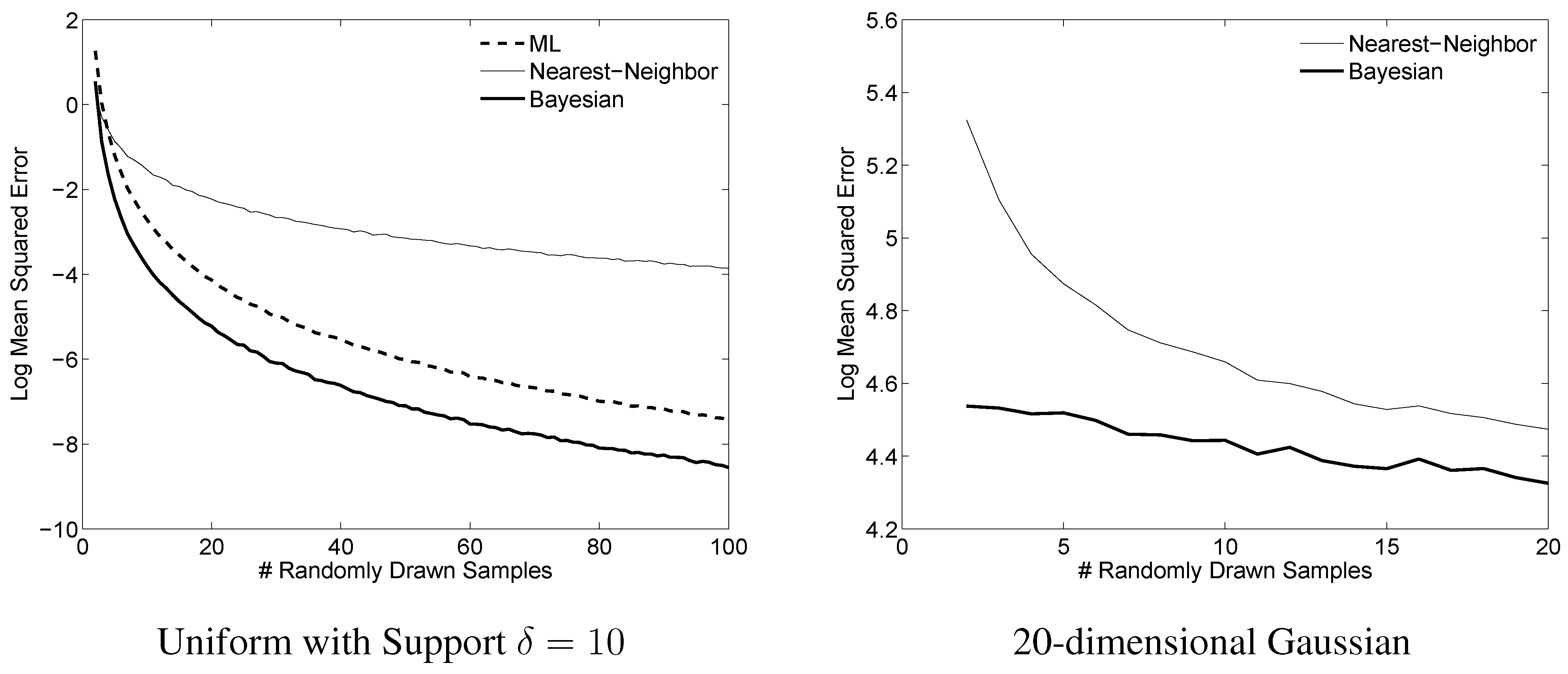
To illustrate the effectiveness of the proposed Bayesian estimates, we show example results from two representative experiments in Figure 1.
Figure 1. Example comparison of differential entropy estimators. Left: For each of 10,000 runs of the simulation, n samples were drawn iid from a uniform distribution on [ 5 , 5 ] . The proposed estimate (9) is compared to the maximum likelihood estimate, and to the nearest-neighbor estimate given in (6). Right: For each of 10,000 runs of the simulation, n samples were drawn iid from a Gaussian distribution. For each of the 10,000 runs, a new Gaussian distribution with diagonal covariance was randomly generated by drawing each of the variances iid from a uniform on [ 0 , 1 ] . The Bayesian estimator prior parameters were q = d and B = . 5 q I . The proposed estimate (12) is compared to the only feasible estimator for this range of n, the nearest-neighbor estimate given in (6).
Entropy 12 00818 g001

4.2. Pareto Prior Knowledge About the Uniform

We consider the case that one has prior knowledge about the random uniform distribution U, where that prior knowledge is formulated as an independent Pareto prior for each dimension such that the prior probability of the marginal ith-dimension uniform U ˜ δ with support of length δ is:
p i ( U ˜ δ ) = α i i α i δ α i + 1 for δ i 0 otherwise
where α i R + and i R + are the Pareto distribution prior parameters for the ith dimension. The parameter i defines the minimum length one believes the uniform’s support could be in the ith dimension, and the parameter α i specifies the confidence that i is the right length; a larger α i means one is more confident that i is the correct length.
Then the differential entropy estimate for the ith dimension’s one-dimensional uniform is:
E U [ h ( U ) ] i = ln Δ i + 1 n + α i + 1 n + α i + 1 , for Δ i i ln i + 1 ( n + α i ) + ( n + α i ) 2 i Δ i i + 1 n + α i + 1 for Δ i < i
Note that the two cases given above do coincide for the boundary case that i = Δ i , so that this differential entropy estimate is a continuous function of Δ i . For the full d-dimensional uniform, the differential entropy estimate is the sum of the one-dimensional differential entropy estimates: i = 1 d E U [ h ( U ) ] i .

5. Gaussian Distribution

The Gaussian is a popular model and often justified by central limit theorem arguments and because it is the maximum entropy distribution given fixed mean and covariance. In this section we assume d-dimensional samples have been drawn iid from an unknown Gaussian N, which we model as a random Gaussian and we take the prior to be an inverse Wishart distribution with scalar parameter q R and parameter matrix B R d × d .
We use the Fisher information metric to define a measure over the Riemannian manifold formed by the set of Gaussian distributions [25,26,27]. We found these choices for prior and measure worked well for estimating Gaussian distributions for Bayesian quadratic discriminant analysis [27].
The performance of the proposed Gaussian entropy and relative entropy estimators will depend strongly on the choice of the prior. Generally, prior knowledge or subjective guesses about the data are used to set the parameters of the prior. Another choice to form a prior is to use a coarse estimate of the data, for example, in previous work we found that setting B equal to the identity matrix times the trace of the sample covariance worked well as a data-adaptive prior in the context of classification [27]. Since the trace times the identity is the extremal case of maximum entropy Gaussian for a given trace, this specific approach is problematic as a coarse estimate for setting the prior for differential entropy estimation, but other coarse estimates based on a different statistic of the eigenvalue may work well.

5.1. Differential Entropy Estimate of the Gaussian Distribution

Assume n samples { x 1 , x 2 , , x n } have been drawn iid from an unknown d-dimensional normal distribution. Per Proposition 1, we estimate the differential entropy as: E N [ h ( N ) ] , where the expectation is taken with respect to the posterior distribution over N and the prior is taken to be inverse Wishart with matrix parameter B R d × d and scale parameter q R . See the appendix for full details and derivation. The resulting estimate is,
E N [ h ( N ) ] = d ln π 2 + ln S + B 2 1 2 i = 1 d ψ n + q + i + 1 2
This estimate is well-defined for any number of samples n.

5.2. Relative Entropy Estimate between Gaussian Distributions

Assume n 1 samples have been drawn iid from an unknown d-dimensional normal distribution N 1 , and n 2 samples have been drawn iid from another d-dimensional distribution N 2 , assumed independent from the first. Then following Proposition 1, we estimate the relative entropy as E N 1 , N 2 [ k l ( N 1 N 2 ) ] where N 1 and N 2 are independent random Gaussians, the expectation is taken with respect to their posterior distributions, and the prior distributions are taken to be inverse Wisharts with scale parameters q 1 and q 2 and matrix parameters B 1 and B 2 . See the appendix for full details and derivation. The resulting estimate is,
E N 1 , N 2 [ k l ( N 1 N 2 ) ] = 1 2 n 2 + q 2 + d + 1 n 1 + q 1 tr ( ( S 1 + B 1 ) ( S 2 + B 2 ) 1 ) 1 2 log | S 1 + B 1 | | S 2 + B 2 | + 1 2 i = 1 d ψ n 2 + q 2 + 1 + i 2 ψ n 1 + q 1 + 1 + i 2 d 2 + 1 2 ( n 2 + q 2 + d + 1 ) tr ( ( S 2 + B 2 ) 1 ( x ¯ 1 x ¯ 2 ) ( x ¯ 1 x ¯ 2 ) T )
This estimate is well-defined for any number of samples n 1 , n 2 . If the prior scalar parameters are taken to be the same, that is q 1 = q 2 , then the digamma terms cancel.

6. Wishart and Inverse Wishart Distributions

The Wishart and inverse Wishart distributions are arguably the most popular distributions for modeling random positive definite matrices. Moreover, if a random variable has a Gaussian distribution, then its sample covariance is drawn from a Wishart distribution. The relative entropy between Wishart distributions may be a useful way to measure the dissimilarity between collections of covariance matrices or Gram (inner product) matrices.
We were unable to find expressions for differential entropy or relative entropy of the Wishart and inverse Wishart distributions, so we first present those, and then present Bayesian estimates of these quantities.

6.1. Wishart Differential Entropy and Relative Entropy

The differential entropy of W is
h ( W ) = ln Γ d q 2 + q d 2 + d + 1 2 ln | 2 Σ | q d 1 2 i = 1 d ψ q d + i 2
The relative entropy between two Wishart distributions p 1 and p 2 with parameters ( q 1 , Σ 1 ) and ( q 2 , Σ 2 ) respectively is,
k l ( p 1 | | p 2 ) = ln Γ d q 2 2 Γ d q 1 2 + q 1 2 tr Σ 1 Σ 2 1 q 1 d 2 q 2 2 ln | Σ 1 Σ 2 1 | q 2 q 1 2 i = 1 d ψ q 1 d + i 2
For the special case of q 1 = q 2 = q , we note that the relative entropy given in (15) is q / 2 times Stein’s loss function, which is itself a common Bregman divergence.
For the special case of Σ 1 = Σ 2 , we find that the relative entropy between two Wisharts can also be written in the form a Bregman divergence [21] between q 2 and q 1 . Consider the strictly convex function ϕ ( q ) = ln Γ d ( q / 2 ) for q R + d , and let ψ d be the derivative of the Γ d . Then (15) becomes,
= ln Γ d q 2 2 ln Γ d q 1 2 q 2 q 1 2 ψ d q 2 2 = ϕ ( q 2 ) ϕ ( q 1 ) ( q 2 q 1 ) ϕ ( q 1 ) = d ϕ ( x , y ) .
We term (16) the log-gamma Bregman divergence. We have not seen this divergence noted before, and hypothesize that this divergence may have physical or practical significance because of the widespread occurrence of the gamma function and its special properties [28].

6.2. Inverse Wishart Differential Entropy and Relative Entropy

Let V be distributed according to an inverse Wishart distribution with scalar degree of freedom parameter q d and positive definite matrix parameter Σ R d × d as per (2).
Then V has differential entropy
h ( V ) = ln Γ d q 2 + q d 2 + d + 1 2 ln Σ 2 q + d + 1 2 i = 1 d ψ q d + i 2
The relative entropy between two inverse Wishart distributions with parameters Σ 1 , q 1 and Σ 2 , q 2 is
ln Γ d q 2 2 Γ d q 1 2 + q 1 2 tr ( Σ 1 1 Σ 2 ) q 1 d 2 q 2 2 ln | Σ 1 1 Σ 2 | q 2 q 1 2 i = 1 d ψ q 1 d + i 2
One sees that the relative entropy between two inverse Wishart distributions is the same as the relative entropy between two Wishart distributions with inverse matrix parameters S 1 1 and S 2 1 respectively. Like the Wishart distribution relative entropy, the inverse Wishart distribution relative entropy has special cases that are the Stein loss and the log-gamma Bregman divergence.

6.3. Bayesian Estimation of Wishart Differential Entropy

We present a Bayesian estimate of the differential entropy of a Wishart distribution p where we make the simplifying assumption that the scalar parameter q is known or estimated (for example, it is common to assume that q = d ). We estimate the differential entropy E Σ [ h ( p ) ] where the estimation is with respect to the uncertainty in the matrix parameter Σ. We assume the prior p ( Σ = Σ ˜ ) is inverse Wishart with scale parameter r and parameter matrix U, which reduces to the non-informative prior when r and U are chosen to be zeros.
Then given sample d × d matrices S 1 , S 2 , , S n drawn iid from the Wishart W, the normalized posterior distribution p ( Σ ˜ | S 1 , S 2 , , S n ) is inverse Wishart with matrix parameter j = 1 n S j + U and scalar parameter n q + r (details in Appendix).
Then our differential entropy estimate E Σ [ h ( W ) ] where the expectation is with respect to the posterior p ( Σ ˜ | { S j } ) is:
ln Γ d q 2 + q d 2 + d + 1 2 ln U + j = 1 n S j d + 1 2 i = 1 d ψ n q + r d + i 2 q d 1 2 i = 1 d ψ q d + i 2

6.4. Bayesian Estimation of Relative Entropy between Two Wisharts

We present a Bayesian estimate of the relative entropy between two Wishart distributions p 1 and p 2 where we make the simplifying assumption that the respective scalar parameters q 1 , q 2 are known or estimated (for example, that q 1 = q 2 = d ), and then we estimate the relative entropy k l ( p 1 | | p 2 ) where the estimation is with respect to the uncertainty in the respective matrix parameters Σ 1 , Σ 2 . To this end, we treat the unknown Wishart parameters Σ 1 , Σ 2 as random, and compute the estimate E Σ 1 , Σ 2 [ k l ( p 1 | | p 2 ) ] . For Σ 1 and Σ 2 we use independent inverse Wishart conjugate priors with respective scalar parameters r 1 , r 2 and parameter matrices U 1 , U 2 , which reduces to non-informative priors when r 1 , r 2 and U 1 , U 2 are chosen to be zeros.
Then given n 1 sample d × d matrices { S j } drawn iid from the Wishart p 1 , and n 2 sample d × d matrices { S k } drawn iid from the Wishart p 2 , the normalized posterior distribution p ( Σ ˜ 1 | { S j } ) is inverse Wishart with matrix parameter j = 1 n 1 S j + U 1 and scalar parameter n 1 q + r 1 , and the normalized posterior distribution p ( Σ 2 ˜ | { S k } ) is inverse Wishart with matrix parameter k = 1 n 2 S k + U 2 and scalar parameter n 2 q + r 2 .
Then our relative entropy estimate E Σ 1 , Σ 2 [ k l ( p 1 | | p 2 ) ] (where the expectation is with respect to the posterior distributions) is
ln Γ d q 2 2 Γ d q 1 2 q 2 q 1 2 i = 1 d ψ q 1 d + i 2 q 1 d 2 + q 1 ( r 1 + n 1 q 1 ) 2 ( r 2 + n 2 q 2 d 1 ) tr ( U 1 + j = 1 n 1 S j ) ( U 2 + k = 1 n 2 S k ) 1 q 2 2 ln | U 1 + j = 1 n 1 S j | + q 2 2 ln | U 2 + k = 1 n 2 S k | q 2 2 i = 1 d ψ n 2 q 2 + r 2 d + i 2 ψ n 1 q 1 + r 1 d + i 2

6.5. Bayesian Estimation of Inverse Wishart Differential Entropy

Let S i denote the ith of n random iid draws from an inverse unknown Wishart distribution p with parameters ( Σ , q ) . Taking the prior p ( Σ ˜ ) to be a Wishart distribution with parameter r and U, our Bayesian estimate of the inverse Wishart differential entropy is
ln Γ d q 2 + q d 2 + d + 1 2 ln | U 1 + j S j 1 | + d + 1 2 i = 1 d ψ n q + r d + i 2 q + d + 1 2 i = 1 d ψ q d + i 2

6.6. Bayesian Estimation of Relative Entropy between Two Inverse Wisharts

Given q 1 , q 2 , and assuming independent Wishart priors with respective scalar parameters r 1 , r 2 and parameter matrices U 1 , U 2 , and given n 1 sample d × d matrices { S j } drawn iid from the inverse Wishart p 1 , and n 2 sample d × d matrices { S k } drawn iid from the inverse Wishart p 2 , our Bayesian estimate of the relative entropy is
ln Γ d q 2 2 Γ d q 1 2 + q 1 2 n 2 q 2 + r 2 n 1 q 1 + r 1 d 1 tr U 1 1 + j = 1 n 1 S j 1 1 U 2 1 + k = 1 n 2 S k 1 q 1 d 2 q 2 2 ln | U 2 1 + k = 1 n 2 S k 1 | | U 1 1 + j = 1 n 1 S j 1 | q 2 q 1 2 i = 1 d ψ q 1 d + i 2 q 2 2 i = 1 d ψ n 2 q 2 + r 2 d + i 2 ψ n 1 q 1 + r 1 d + i 2

7. Discussion

We have presented Bayesian differential entropy and relative entropy estimates for four standard distributions, and in doing so illustrated techniques that could be used to derive such estimates for other distributions. For the uniform case with no prior, the given estimators perform significantly better than previous estimators, and this experimental evidence validates our approach. However given a prior over distributions, the performance will depend heavily on the accuracy of the prior, and a thorough experimental study would be useful to practitioners but was outside the scope of this investigation.
In practice, there may not be a priori information available to determine a prior, and an open question is how to design appropriate data-dependent priors for differential entropy estimation. For example, for Bayesian quadratic discriminant analysis classification [27], we have shown that setting the prior matrix parameter for the Gaussian to be a coarse estimate of the data’s covariance (the identity times the trace of the sample covariance) works well. However, for differential entropy estimation the trace forms an extreme estimate, and is thus not (by itself) suitable for forming a data-dependent prior for this problem.
Another open area is forming estimators for more complicated parametric models, for example estimating the differential entropy and relative entropy of Gaussian mixture models. Estimating the differential entropy of Gaussian processes is also an important problem [29] that may be amenable to the present approach.
Lastly, the new estimators have been motivated by their expected Bregman loss optimality and by the practical consideration of producing estimates even when there are fewer samples than dimensions, but there are a number of theoretical questions about these estimators that are open, such as domination.

Acknowledgments

We would like to thank the United States Office of Naval Research for funding this research.

References

  1. El Saddik, A.; Orozco, M.; Asfaw, Y.; Shirmohammadi, S.; Adler, A. A novel biometric system for identification and verification of haptic users. IEEE Trans. Instrum. Meas. 2007, 56, 895–906. [Google Scholar] [CrossRef]
  2. Choi, H. Adaptive Sampling and Forecasting with Mobile Sensor Networks . PhD Dissertation, MIT, Cambridge, MA, USA, 2009. [Google Scholar]
  3. Moddemeijer, R. On estimation of entropy and mutual information of continuous distributions. Signal Process. 1989, 16, 233–246. [Google Scholar] [CrossRef]
  4. Misra, N.; Singh, H.; Demchuk, E. Estimation of the entropy of a multivariate normal distribution. J. Multivariate Anal. 2005, 92, 324–342. [Google Scholar] [CrossRef]
  5. Wang, Q.; Kulkarni, S.R.; Verdú, S. Divergence estimation for multi-dimensional densities via k nearest-neighbor distances. IEEE Trans. Inform. Theory 2009, 55, 2392–2405. [Google Scholar] [CrossRef]
  6. Ahmed, N.A.; Gokhale, D.V. Entropy expressions and their estimators for multivariate distributions. IEEE Trans. Inform. Theory 1989, 688–692. [Google Scholar] [CrossRef]
  7. Beirlant, J.; Dudewicz, E.; Györfi, L.; Meulen, E.V.D. Nonparametric entropy estimation: An overview. Intl. J. Math. Stat. Sci. 1997, 6, 17–39. [Google Scholar]
  8. Nilsson, M.; Kleijn, W.B. On the estimation of differential entropy from data located on embedded manifolds. IEEE Trans. Inform. Theory 2007, 53, 2330–2341. [Google Scholar] [CrossRef]
  9. Kozachenko, L.F.; Leonenko, N.N. Sample estimate of entropy of a random vector. Probl. Inform. Transm. 1987, 23, 95–101. [Google Scholar]
  10. Goria, M.N.; Leonenko, N.N.; Mergel, V.V.; Inverardi, P.L. A new class of random vector entropy estimators and its applications in testing statistical hypotheses. J. Nonparametric Stat. 2005, 17, 277–297. [Google Scholar] [CrossRef]
  11. Mnatsakanov, R.M.; Misra, N.S.E. kn-Nearest neighbor estimators of entropy. Math. Method. Stat. 2008, 17, 261–277. [Google Scholar] [CrossRef]
  12. Hero, A.; Michel, O. Asymptotic theory of greedy approximations to minimal k-point random graphs. IEEE Trans. Inform. Theory 1999, 45, 1921–1939. [Google Scholar] [CrossRef]
  13. Hero, A.; Ma, B.; Michel, O.; Gorman, J. Applications of entropic spanning graphs. IEEE Signal Process. Mag. 2002, 19, 85–95. [Google Scholar] [CrossRef]
  14. Costa, J.; Hero, A. Geodesic entropic graphs for dimension and entropy estimation in manifold learning. IEEE Trans. Signal Process. 2004, 52, 2210–2221. [Google Scholar] [CrossRef]
  15. Hulle, M.M.V. Edgeworth approximation of multivariate differential entropy. Neural Comput. 2005, 17, 1903–1910. [Google Scholar] [CrossRef] [PubMed]
  16. Wang, Q.; Kulkarni, S.R.; Verdú, S. Divergence estimation of continuous distributions based on data-dependent partitions. IEEE Trans. Inform. Theory 2005, 51, 3064–3074. [Google Scholar] [CrossRef]
  17. Nguyen, X.; Wainwright, M.J.; Jordan, M.I. Estimating divergence functional and the likelihood ratio by penalized convex risk minimization. Advances Neural Inform. Process. Syst. 2007. [Google Scholar]
  18. Wang, Q.; Kulkarni, S.R.; Verdú, S. A nearest-neighbor approach to estimating divergence between continuous random vectors. In Proceedings of the 2006 IEEE International Symposium on Information Theory, Seattle, WA, USA, 9–14 July 2006; IEEE: Washington, DC, USA, 2006. [Google Scholar]
  19. Pérez-Cruz, F. Estimation of information-theoretic measures for continuous random variables. Adv. Neural Inform. Process. Syst. (NIPS) 2009. [Google Scholar]
  20. Lehmann, E.L.; Casella, G. Theory of Point Estimation; Springer: New York, NY, USA, 1998; Chapter 4. [Google Scholar]
  21. Bregman, L. The relaxation method of finding the common points of convex sets and its application to the solution of problems in convex programming. USSR Comput. Math. Math. Phys. 1967, 7, 200–217. [Google Scholar] [CrossRef]
  22. Banerjee, A.; Guo, X.; Wang, H. On the optimality of conditional expectation as a Bregman predictor. IEEE Trans. Inform. Theory 2005, 51, 2664–2669. [Google Scholar] [CrossRef]
  23. Jones, L.K.; Byrne, C.L. General entropy criteria for inverse problems, with applications to data compression, pattern classification, and cluster analysis. IEEE Trans. Inform. Theory 1990, 36, 23–30. [Google Scholar] [CrossRef]
  24. Frigyik, B.A.; Srivastava, S.; Gupta, M.R. Functional Bregman divergence and Bayesian estimation of distributions. IEEE Trans. Inform. Theory 2008, 54, 5130–5139. [Google Scholar] [CrossRef]
  25. Amari, S.; Nagaoka, H. Methods of Information Geometry; Oxford University Press: New York, NY, USA, 2000. [Google Scholar]
  26. Kass, R.E. The geometry of asymptotic inference. Stat. Sci. 1989, 4, 188–234. [Google Scholar] [CrossRef]
  27. Srivastava, S.; Gupta, M.R.; Frigyik, B.A. Bayesian quadratic discriminant analysis. J. Mach. Learn. Res. 2007, 8, 1287–1314. [Google Scholar]
  28. Havil, J. Gamma; Princeton University Press: Princeton, NJ, USA, 2003. [Google Scholar]
  29. Bercher, J.; Vignat, C. Estimating the entropy of a signal with applications. IEEE Trans. Signal Process. 2000, 48, 1687–1694. [Google Scholar] [CrossRef]
  30. Bilodeau, M.; Brenner, D. Theory of Multivariate Statistics; Springer Texts in Statistics: New York, NY, USA, 1999. [Google Scholar]

Appendix

A.1. Proof of Proposition 1

The proof is by contradiction. Let ξ * = E A [ ξ ( A ) ] , and assume the true minimizer of E A d ϕ ( ξ ( A ) , ξ ^ ) occurs instead at some other value s. Then a contradiction occurs:
E A d ϕ ( ξ ( A ) , s ) E A d ϕ ( ξ ( A ) , ξ * ) = ( a ) ϕ ( ξ * ) ϕ ( s ) d ϕ ( s ) d s ( E A [ ξ ( A ) ] s ) + d ϕ ( ξ * ) d ξ * ( E A [ ξ ( A ) ] ξ * ) = ( b ) ϕ ( ξ * ) ϕ ( s ) d ϕ ( s ) d s ( E A [ ξ ( A ) ] s ) = ( c ) d ϕ ( ξ * , s ) ( d ) 0
where in ( a ) we expanded d ϕ and simplified, in ( b ) we used the fact that ξ * = E A [ ξ ( A ) ] , in ( c ) we substituted ξ * = E A [ ξ ( A ) ] and used the definition of the Bregman divergence, and in ( d ) we used the non-negativity of the Bregman divergence. Thus ξ * = E A [ ξ ( A ) ] must be the minimizer.

A.2. Derivation of Uniform Differential Entropy Estimate

In this section we will repeatedly use the integral:
ln u u m d u = ln u ( m 1 ) u m 1 1 ( m 1 ) 2 u m 1
To estimate the differential entropy of a multidimensional uniform distribution one only needs to consider the differential entropy for a one-dimensional uniform, because a multidimensional uniform can be written as a product of independent univariate distributions, and thus the differential entropy of the multidimensional uniform is the sum of the univariate entropies.
Thus we model the n samples { x 1 , x 2 , , x n } as being drawn from a random one-dimensional uniform distribution U. Let M be the two-dimensional statistical manifold composed of uniform distributions { U ˜ a , b } , where U ˜ a , b has support on [ a , b ] for b > a , a , b , R . The measure should depend on the length δ = b a of the uniform and be invariant to shifts in the support. To that end, we use the Fisher information metric [25,26] based on the length,
d M = | I ( δ ) | 1 / 2 d δ = d δ δ
where I is the Fisher information matrix,
I ( δ ) = E X d 2 log 1 δ d δ 2 = 1 δ 2
Using d M as a differential element and the normalized likelihood of the samples for p ( U ˜ a , b ) , the uniform differential entropy estimate is
E U [ h ( U ) ] = M h ( U ˜ a , b ) p ( U ˜ a , b ) d M M p ( U ˜ a , b ) d M = 1 γ a = x min b = x max ln ( b a ) ( b a ) n d a d b ( b a ) = 1 γ n ( n 1 ) ( x max x min ) n 1 ln ( x max x min ) + 1 n 1 + 1 n
where the normalization factor γ is
γ = a = x min b = x max 1 ( b a ) n d a d b ( b a ) = 1 ( n 1 ) n ( x max x min ) n 1
Canceling terms in (23) due to the normalization factor γ yields the one-dimensional uniform differential entropy ln ( x max x min ) + 1 n 1 + 1 n . For the multidimensional uniform, one sums these marginal entropy terms over the dimensions, as given in (9).

A.3. Derivation of Uniform differential Entropy Given Pareto Prior

As explained for the no-prior derivation, we need only consider a one-dimensional uniform. Although the Pareto distribution is a conjugate prior for the uniform with respect to its length, one must be careful because the data restrict b > x max and a < x min , and these restrictions are not taken into account if one integrates with respect to the variable δ. Throughout this section we use various flavors of γ to denote normalization constants, and Δ = x max x min . We consider two cases separately.
Case I: Δ :
p ( U ˜ a , b | { x i } ) = 1 γ 1 p ( { x i } | U ˜ a , b ) p ( U ˜ a , b ) = 1 γ 1 α α ( b a ) n + α + 1 for a x min , b x max 0 otherwise ,
where the normalizer is
γ 1 = a = x min b = x max p ( { x i } | U ˜ a , b ) p ( U ˜ a , b ) d a d b b a = a = x min b = x max α α ( b a ) n + α + 1 d a d b b a = α α ( n + α + 1 ) ( n + α ) Δ n + α
Then the posterior (24) becomes,
p ( U ˜ a , b | { x i } ) = ( n + α ) ( n + α + 1 ) Δ n + α ( b a ) n + α + 1 for a x min , b x max 0 otherwise .
Using (22), it is straightforward to derive the differential entropy estimate given in the text as:
E U [ h ( U ) ] = ( n + α ) ( n + α + 1 ) Δ n + α a = x min b = x max ln ( b a ) ( b a ) n + α + 1 d a d b b a = ln Δ + 1 n + α + 1 n + α + 1
Case II: > Δ :
In this case, the posterior has an additional constraint compared to (24):
p ( U ˜ a , b | { x i } ) = 1 γ 2 p ( { x i } | U ˜ a , b ) p ( U ˜ a , b ) = 1 γ 2 α α ( b a ) n + α + 1 for a x min , b x max , and b a 0 otherwise .
The normalization constant can be solved for as:
γ 2 = a = x min b = x max p ( { x i } | U ˜ a , b ) p ( U ˜ a , b ) d a d b b a = a = x max b = x max α α ( b a ) n + α + 1 d a d b b a + a = x max x min b = a + α α ( b a ) n + α + 1 d a d b b a = α α ( n + α + 1 ) ( n + α ) n + α + α α ( Δ ) ( n + α + 1 ) n + α + 1 = α α ( n + α + 1 ) n + α 1 n + α + Δ
Then the differential entropy estimate is
E U [ h ( U ) ] = α α γ 2 a = x max b = x max ln ( b a ) ( b a ) n + α + 1 d a d b b a + a = x max x min b = a + ln ( b a ) ( b a ) n + α + 1 d a d b b a = α α γ 2 ln ( n + α + 1 ) ( n + α ) n + α + 1 ( n + α + 1 ) ( n + α ) 2 n + α + 1 ( n + α ) ( n + α + 1 ) 2 n + α + α α γ 2 ( Δ ) ln ( n + α + 1 ) n + α + 1 + Δ ( n + α + 1 ) 2 n + α + 1 = α α γ 2 ( n + α + 1 ) n + α ln ( n + α ) + 1 ( n + α ) 2 + 1 ( n + α ) ( n + α + 1 ) + ( Δ ) ln + Δ ( n + α + 1 ) = ( a ) ( n + α ) + ( n + α ) ( Δ ) · ln ( n + α ) + 1 ( n + α ) 2 + 1 ( n + α ) ( n + α + 1 ) + ( Δ ) ln + Δ ( n + α + 1 )
where in ( a ) we substituted in (25). In the second factor of ( a ) there are five terms. Combining the first and fourth term with the first factor results in the first term of the estimate given in (11). Combining the second term with the first factor results in the second term of (11). Lastly, combining the third and fifth term of ( a ) with the first factor results in the third term of (11).

A.4. Propositions Used in Remaining Derivations

The following identities and propositions will be used repeatedly in the derivations in the rest of the appendix.
Identity 1.
This is a convenient re-statement of the fact that the normal distribution normalizes to one. For x , μ R d and positive definite d × d matrix Σ,
μ e n 2 tr Σ 1 ( x μ ) ( x μ ) T d μ = 2 π n d 2 | Σ | 1 2
Identity 2.
This is a convenient re-statement of the fact that the inverse Wishart distribution normalizes to one. For positive definite Σ:
Σ > 0 e tr Σ 1 B | Σ | q 2 d Σ = Γ d q d 1 2 | B | q d 1 2
Proposition 2.
For W Wishart ( S , q ) ,
E [ ln | W | ] = ln | S | + d ln 2 + i = 1 d ψ q d + i 2 ln | 2 S | + i = 1 d ψ q d + i 2
Proof:
Recall that | W | is distributed as | S | i = 1 d χ q d + i 2 ([30, Corollary 7.3]) where χ 2 denotes the chi-squared random variable. Then the result is produced by taking the expected log and using the fact that E [ ln χ q 2 ] = ln 2 + ψ q 2 [4]. Lastly the equivalence follows because ln | 2 S | = ln 2 d | S | = d ln 2 + ln | S | .
Proposition 3.
For V inverse Wishart ( S , q ) ,
E [ ln | V | ] = ln | S | d ln 2 i = 1 d ψ q d + i 2 ln S 2 i = 1 d ψ q d + i 2
Proof:
Let Z = V 1 , then Z Wishart ( S 1 , q ) , and E [ ln | V | ] = E [ ln | Z | 1 ] = E [ ln | Z | ] = ln | S 1 | d ln 2 i = 1 d ψ q d + i 2 , by Proposition 2, and noting that ln | S 1 | = ln | S | produces the result. Lastly, the equivalence follows because ln | S 2 | = ln 1 2 d | S | = d ln 2 + ln | S | .
Proposition 4.
For W Wishart ( S , q ) and any positive definite matrix A R d × d ,
E [ tr ( W A ) ] = q tr ( S A )
Proof:
E [ tr ( W A ) ] = tr ( E [ W ] A ) = q tr ( S A ) .
Proposition 5.
For V inverse Wishart ( S , q ) and any positive definite matrix A R d × d ,
E [ tr ( V A ) ] = tr ( A S ) q d 1
Proof:
E [ tr ( V A ) ] = tr ( E [ V ] A ) = tr ( A S ) / ( q d 1 ) .
Proposition 6.
For V inverse Wishart ( S , q ) and any positive definite matrix A R d × d ,
E [ tr ( V 1 A ) ] = q tr ( S 1 A )
Proof:
By definition, V 1 Wishart ( S 1 , q ) , and so one can apply Proposition 4 to yield E [ tr ( V 1 A ) ] = q tr ( S 1 A ) .

A.5. Derivation of Bayesian Gaussian Differential Entropy Estimate

We model the samples { x i } i = 1 n as being drawn from a random d-dimensional normal distribution N and assume an inverse Wishart prior distribution for N with parameters ( B , q ) . That is, the prior probability that the random normal N is N ˜ ( μ ˜ , Σ ˜ ) is
p ( N = N ˜ ( μ ˜ , Σ ˜ ) ) = | B | q 2 e 1 2 tr Σ ˜ 1 B 2 q d 2 Γ q 2 | Σ ˜ | q + d + 1 2
The likelihood can be written:
p ( { x i } i = 1 n | N = N ˜ ( μ ˜ , Σ ˜ ) ) = 1 2 π n d 2 | Σ ˜ | n 2 i = 1 n e 1 2 tr Σ ˜ 1 ( x i μ ˜ ) ( x i μ ˜ ) T = 1 2 π n d 2 | Σ ˜ | n 2 e 1 2 i = 1 n tr Σ ˜ 1 ( x i x ¯ + x ¯ μ ˜ ) ( x i x ¯ + x ¯ μ ˜ ) T = 1 2 π n d 2 | Σ ˜ | n 2 e 1 2 tr Σ ˜ 1 S n 2 tr Σ ˜ 1 ( x ¯ μ ˜ ) ( x ¯ μ ˜ ) T
Then the posterior is the likelihood times the prior normalized, or sweeping all the constant terms into a normalization term α we can write the posterior as:
p ( N = N ˜ ( μ ˜ , Σ ˜ ) | { x i } i = 1 n ) = 1 α e 1 2 tr Σ ˜ 1 S n 2 tr Σ ˜ 1 ( x ¯ μ ˜ ) ( x ¯ μ ˜ ) T | Σ ˜ | n 2 e 1 2 tr Σ ˜ 1 B | Σ ˜ | q + d + 1 2
Note that this is a density on the statistical manifold of Gaussians, so we integrate with respect to the Fisher information measure 1 / | Σ ˜ | d + 2 2 [27], [25,] rather than the Lebesgue measure, such that
α = Σ ˜ μ ˜ e n 2 tr Σ ˜ 1 ( x ¯ μ ˜ ) ( x ¯ μ ˜ ) T | Σ ˜ | n + q + d + 1 2 e 1 2 tr Σ ˜ 1 ( S + B ) d Σ ˜ d μ ˜ | Σ ˜ | d + 2 2 = 2 π n d 2 Γ d n + q + d + 1 2 | S + B | n + q + d + 1 2 2 d ( n + q + d + 1 ) 2
where the last line follows from Identities 1 and 2 stated in the previous subsection.
Then combining (30) and (29), the posterior is:
p ( N = N ˜ ( μ ˜ , Σ ˜ ) | { x i } i = 1 n ) = n 2 π d 2 | S + B | n + q + d + 1 2 Γ d n + q + d + 1 2 1 2 d ( n + q + d + 1 ) 2 e 1 2 tr Σ ˜ 1 ( S + B ) n 2 tr Σ ˜ 1 ( x ¯ μ ˜ ) ( x ¯ μ ˜ ) T | Σ ˜ | n + q + d + 1 2
Our differential entropy estimate is the integral E N [ h ( N ) ] , which is an integral over the statistical manifold of Gaussians that we convert to an integral over covariance matrices by using the Fisher information metric 1 / | Σ ˜ | ( d + 2 ) / 2 [27], [25,]. Then,
E N [ h ( N ) ] = N ˜ ( μ ˜ , Σ ˜ ) d 2 + d ln ( 2 π ) 2 + ln | Σ ˜ | 2 p ( N ˜ ( μ ˜ , Σ ˜ ) | { x i } ) d N ˜ = d 2 + d ln ( 2 π ) 2 + n 2 π d 2 | S + B | n + q + d + 1 2 2 2 + d ( n + q + d + 1 ) 2 Γ d n + q + d + 1 2 Σ ˜ > 0 μ ˜ ln | Σ ˜ | e 1 2 tr Σ ˜ 1 ( S + B ) n 2 tr Σ ˜ 1 ( x ¯ μ ˜ ) ( x ¯ μ ˜ ) T | Σ ˜ | n + q + d + 1 2 d Σ ˜ d μ ˜ | Σ ˜ | d + 2 2
We evaluate the third term of (32) as follows:
n 2 π d 2 | S + B | n + q + d + 1 2 2 2 + d ( n + q + d + 1 ) 2 Γ d n + q + d + 1 2 Σ ˜ > 0 ln | Σ ˜ | e 1 2 tr Σ ˜ 1 ( S + B ) | Σ ˜ | n + q + 2 d + 3 2 μ ˜ e n 2 tr Σ ˜ 1 ( x ¯ μ ˜ ) ( x ¯ μ ˜ ) T d μ ˜ d Σ ˜
= n 2 π d 2 | S + B | n + q + d + 1 2 2 2 + d ( n + q + d + 1 ) 2 Γ d n + q + d + 1 2 Σ ˜ > 0 ln | Σ ˜ | e 1 2 tr Σ ˜ 1 ( S + B ) | Σ ˜ | n + q + 2 d + 3 2 2 π n d 2 | Σ ˜ | 1 2 d Σ ˜
= | S + B | n + q + d + 1 2 2 2 + d ( n + q + d + 1 ) 2 Γ d n + q + d + 1 2 Σ ˜ > 0 ln | Σ ˜ | e 1 2 tr Σ ˜ 1 ( S + B ) | Σ ˜ | n + q + 2 d + 2 2 d Σ ˜
= 1 2 ln | S + B | d 2 ln 2 1 2 i = 1 d ψ n + q + 1 + i 2
where (33) follows by Integral Identity 1; and (34) is half the expectation of ln | Σ | with respect to the inverse Wishart with parameters ( S + B , n + q + d + 1 ) , and thus (35) follows from (34) by Proposition 3.
Then (32) becomes
d 2 + d ln π 2 + 1 2 ln | S + B | 1 2 i = 1 d ψ n + q + 1 + i 2

A.6. Derivation of Bayesian Gaussian Relative Entropy Estimate

Recall that the relative entropy between independent Gaussians N 1 ( x ; μ 1 , Σ 1 ) and N 2 ( x ; μ 2 , Σ 2 ) is
K L ( N 1 N 2 ) = 1 2 tr ( Σ 1 Σ 2 1 ) log | Σ 1 Σ 2 1 | d + tr Σ 2 1 ( μ 1 μ 2 ) ( μ 1 μ 2 ) T
Here we derive E N 1 , N 2 [ K L ( N 1 N 2 ) ] . Analogous to the previous derivation of the Bayesian Gaussian entropy estimate, we form the posterior distributions using independent inverse Wishart priors with parameters ( B 1 , q 1 ) and ( B 2 , q 2 ) . (Note that this is equivalent to having a non-informative prior on the mean parameter, and that a different prior on the mean would lead to a more regularized estimate). We consider the four terms of the expectation of (37), that is, of E N 1 , N 2 [ K L ( N 1 N 2 ) ] , in turn.
The first term is:
E N 1 , N 2 tr ( Σ 1 Σ 2 1 ) = tr ( Σ 1 Σ 2 1 ) p ( N ˜ 1 ( μ ˜ 1 , Σ ˜ 1 ) | { x 1 , i } i = 1 n 1 ) p ( N ˜ 2 ( μ ˜ 2 , Σ ˜ 2 ) | { x 2 , i } i = 1 n 2 ) d N ˜ 1 d N ˜ 2
where the posteriors are given by (31). Using the Fisher information measure as above, (38) can be re-written as expectations of functions of independent random covariance matrices Σ 1 , Σ 2 drawn from inverse Wishart distributions with respective parameters ( S 1 + B 1 , n 1 + q 1 + d + 1 ) and ( S 2 + B 2 , n 2 + q 2 + d + 1 ) :
E Σ 1 , Σ 2 tr ( Σ 1 Σ 2 1 ) = ( a ) 1 n 1 + q 1 E Σ 2 tr ( ( S 1 + B 1 ) Σ 2 1 ) , = ( b ) n 2 + q 2 + d + 1 n 1 + q 1 tr ( ( S 1 + B 1 ) ( S 2 + B 2 ) 1 )
where ( a ) is by Proposion 5, and ( b ) is by Proposition 6.
Similarly, we can write the second term as:
E Σ 1 , Σ 2 log | Σ 1 Σ 2 1 | = E Σ 1 , Σ 2 log | Σ 1 | log | Σ 2 | = E Σ 1 log | Σ 1 | E Σ 2 log | Σ 2 | = log | S 1 + B 1 | | S 2 + B 2 | + i = 1 d ψ n 2 + q 2 + 1 + i 2 ψ n 1 + q 1 + 1 + i 2
where the last line follows from Proposition 4.
The third term is simply d . The fourth term simplifies by Proposition 6 to:
E Σ 2 [ tr ( Σ 2 1 ( x ¯ 1 x ¯ 2 ) ( x ¯ 1 x ¯ 2 ) T ) ] = ( n 2 + q 2 + d + 1 ) tr ( ( S 2 + B 2 ) 1 ( x ¯ 1 x ¯ 2 ) ( x ¯ 1 x ¯ 2 ) T )
Combining the terms yields the relative entropy estimate given in (13).

A.7. Derivation of Wishart Differential Entropy:

Using the Wishart density given in (1), the Wishart differential entropy h ( W ) is E [ ln p ( W ) ] ,
= q d 2 ln 2 + q 2 ln | Σ | + ln Γ d q 2 + 1 2 E [ tr ( W Σ 1 ) ] q d 1 2 E [ ln | W | ] , = ( a ) q d 2 ln 2 + q 2 ln | Σ | + ln Γ d q 2 + q d 2 q d 1 2 E [ ln | W | ] , = ( b ) q d 2 ln 2 + q 2 ln | Σ | + ln Γ d q 2 + q d 2 q d 1 2 ln | Σ | + d ln 2 + i = 1 d ψ q d + i 2 , = ( c ) ln Γ d q 2 + q d 2 + d + 1 2 ln | 2 Σ | q d 1 2 i = 1 d ψ q d + i 2
where ( a ) follows by applying Proposition 4 to show that E [ tr ( W Σ 1 ) ] = q tr ( Σ Σ 1 ) = q d , and then in ( b ) one applies Proposition 2 to E [ ln | W | ] and recalls that ln | 2 Σ | = ln | Σ | + d ln 2

A.8. Derivation of Wishart Relative Differential Entropy:

The relative entropy k l ( p 1 , p 2 ) is
= E p 1 [ ln p 1 ( W ) p 2 ( W ) ] = h ( p 1 ) E p 1 [ ln p 2 ( W ) ] = ( a ) ln Γ d q 1 2 q 1 d 2 d + 1 2 ln | 2 Σ 1 | + q 1 d 1 2 i = 1 d ψ q 1 d + i 2 q 2 d 1 2 E p 1 [ ln | W | ] + 1 2 E p 1 [ tr ( W Σ 2 1 ) ] + q 2 2 ln | 2 Σ 2 | + ln Γ d q 2 2 = ( b ) ln Γ d q 2 2 Γ d q 1 2 + q 1 2 tr Σ 1 Σ 2 1 q 1 d 2 q 2 2 ln | Σ 1 Σ 2 1 | q 2 q 1 2 i = 1 d ψ q 1 d + i 2
where ( a ) uses the formula for entropy given in (14), and ( b ) follows by applying Proposition 2 and 4 and then simplifying.

A.9. Derivation of Inverse Wishart Differential Entropy:

Using the inverse Wishart density given in (2), the inverse Wishart differential entropy is:
h ( V ) = q 2 ln | S | + E [ tr ( V 1 S ) ] 2 + q d 2 ln 2 + ln Γ d q 2 + q + d + 1 2 E [ ln | V | ] = ( a ) q 2 ln | S | + q tr ( S 1 S ) 2 + q d 2 ln 2 + ln Γ d q 2 + q + d + 1 2 ln | S | d ln 2 i = 1 d ψ q d + i 2 = ( b ) d + 1 2 ln S 2 + q d 2 + ln Γ d q 2 q + d + 1 2 i = 1 d ψ q d + i 2
where in ( a ) we applied Proposition 6 and Proposition 3, and in ( b ) used tr ( S 1 S ) = tr ( I ) = d and simplified.

A.10. Derivation of Inverse Wishart Relative Entropy:

Taking the expectation with respect to the first inverse Wishart V 1 of the log of the ratio of the two inverse Wishart distributions yields
( q 2 q 1 ) 2 d ln 2 + E [ tr ( Σ 2 Σ 1 ) V 1 1 ] 2 q 2 2 ln | Σ 2 | + q 1 2 ln | Σ 1 | + ln Γ d q 2 2 ln Γ d q 1 2 + q 2 q 1 2 E [ ln | V 1 | ] = ( a ) ( q 2 q 1 ) 2 d ln 2 + q 1 tr ( Σ 2 Σ 1 1 ) 2 q 1 d 2 q 2 2 ln | Σ 2 | + q 1 2 ln | Σ 1 | + ln Γ d q 2 2 ln Γ d q 1 2 + q 2 q 1 2 E [ ln | V 1 | ] = ( b ) q 2 q 1 2 d ln 2 + q 1 tr ( Σ 2 Σ 1 1 ) 2 q 1 d 2 q 2 2 ln | Σ 2 | + q 1 2 ln | Σ 1 | + ln Γ d q 2 2 ln Γ d q 1 2 + q 2 q 1 2 ln | Σ 1 | d ln 2 i = 1 d ψ q 1 d + i 2 , = ln Γ d q 2 2 Γ d q 1 2 + q 1 2 tr ( Σ 2 Σ 1 1 ) q 1 d 2 + q 2 2 ln | Σ 1 Σ 2 1 | q 2 q 1 2 i = 1 d ψ q 1 d + i 2
where ( a ) results from distributing the trace and applying Proposition 6 to each term and recalling that tr I = d , ( b ) applies Proposition 3, and the last line is simplifications.

A.11. Derivation of Bayesian Estimate of Wishart Differential Entropy:

Given sample d × d matrices S 1 , S 2 , , S n drawn iid from the unknown Wishart W with unknown parameters Σ , q , the normalized posterior distribution p ( Σ = Σ ˜ | S 1 , S 2 , , S n ) is the normalized product of the inverse Wishart prior p ( Σ ˜ ) and the product of n Wishart likelihoods j p ( S j | Σ ˜ ) . To derive the posterior, we take the product of the prior and likelihood and sweep all terms that do not depend on Σ ˜ into a normalization constant γ:
p ( Σ ˜ | { S j } ) = γ j = 1 n e 1 2 tr ( Σ ˜ 1 S j ) | Σ ˜ | q 2 e 1 2 tr ( Σ ˜ 1 U ) | Σ ˜ | r + d + 1 2 = γ e 1 2 tr Σ ˜ 1 U + j = 1 n S j | Σ ˜ | n q + r + d + 1 2 = | U + j = 1 n S j | n q + r 2 e 1 2 tr Σ ˜ 1 U + j = 1 n S j 2 ( n q + r ) d 2 Γ d n q + r 2 | Σ ˜ | n q + r + d + 1 2
where in (39) we solved for the normalization constant γ. One sees from (39) that the posterior p ( Σ ˜ | { S j } ) is inverse Wishart with parameters U + j S j and n q + r .
Then the differential entropy estimate E [ h ( W ) ] can be computed by taking the expectation of h ( W ) given in (14) where the W is treated as random and the expectation is with respect to the posterior given in (39). Only one term requires the expectation:
E [ ln | 2 Σ | ] = E [ ln | Σ | ] + d ln 2 = ln | j = 1 n S j + U | i = 1 d ψ n q + r d + i 2
where ( b ) applies Proposition 3. Substituting this term into the differential entropy formula (14) produces the differential entropy estimate (19).

A.12. Derivation of Bayesian Estimate of Relative Entropy Between Wisharts:

There are only two terms of (15) that require evaluating the expectation, taken with respect to the independent posteriors of the form given in (39).
The first term is evaluated by applying Proposition 4 and Proposition 5 sequentially:
E Σ 1 , Σ 2 tr Σ 1 Σ 2 1 = ( r 1 + n 1 q 1 ) ( r 2 + n 2 q 2 d 1 ) tr U 1 + j = 1 n 1 S j U 2 + k = 1 n 2 S k 1
The second term follows by applying Proposition 3 twice:
E Σ 1 , Σ 2 ln | Σ 1 Σ 2 1 | = E Σ 1 , Σ 2 ln | Σ 1 | | Σ 2 1 | = E Σ 1 ln | Σ 1 | E Σ 2 ln | Σ 2 | = ln | U 1 + j = 1 n 1 S j | ln | U 2 + k = 1 n 2 S k | + i = 1 d ψ n 2 q 2 + r 2 d + i 2 ψ n 1 q 1 + r 1 d + i 2

A.13. Derivation of Bayesian Estimate of Inverse Wishart Differential Entropy:

Given sample d × d matrices S 1 , S 2 , , S n drawn iid from the unknown inverse Wishart V with unknown parameters Σ , q , the normalized posterior distribution p ( Σ = Σ ˜ | S 1 , S 2 , , S n ) is the normalized product of the Wishart prior p ( Σ ˜ ) and the product of n inverse Wishart likelihoods j p ( S j | Σ ˜ ) .
To derive the posterior, we take the product of the prior and likelihood and sweep all terms that do not depend on Σ ˜ into a normalization constant γ:
p ( Σ ˜ | { S j } ) = γ j = 1 n | Σ ˜ | q 2 e 1 2 tr ( Σ ˜ S j 1 ) | Σ ˜ | r d 1 2 e 1 2 tr ( Σ ˜ U 1 ) = γ | Σ ˜ | n q + r d 1 2 e 1 2 tr Σ ˜ U 1 + j = 1 n S j 1 = | Σ ˜ | n q + r d 1 2 e 1 2 tr Σ ˜ U 1 + j = 1 n S j 1 2 ( n q + r ) d 2 Γ d n q + r 2 | U + j = 1 n S j 1 | n q + r 2
where in (40) we solved for the normalization constant γ. One sees from (40) that the posterior p ( Σ ˜ | { S j } ) is Wishart with parameters U 1 + j S j 1 and n q + r .
Then the differential entropy estimate E [ h ( V ) ] can be computed by taking the expectation of h ( V ) given in (17) where the V is treated as random and the expectation is with respect to the posterior given in (40). Only one term requires the expectation:
E ln | Σ 2 | = ( a ) E [ ln | Σ | d ln 2 = ( b ) ln | U 1 + i S i 1 | + i = 1 d ψ n q + r d + i 2
where ( a ) expands ln | Σ / 2 | = ln | Σ | d ln 2 , and ( b ) applies Proposition 2.
Substituting in this term to the differential entropy formula (17) produces the differential entropy estimate (20).

A.14. Derivation of Bayesian Estimate of Relative Entropy Between Inverse Wisharts:

There are only two terms of (18) that require evaluating the expectation, taken with respect to the independent posteriors of the form given in (40).
The first term is:
E Σ 1 , Σ 2 tr Σ 1 1 Σ 2 = ( a ) ( n 2 q 2 + r 2 ) E Σ 1 tr Σ 1 1 U 2 1 + j = 1 n 2 S 2 j 1 = ( b ) n 2 q 2 + r 2 n 1 q 1 + r 1 d 1 tr U 1 1 + j = 1 n 1 S 1 j 1 1 U 2 1 + j = 1 n 2 S 2 j 1 ,
where ( a ) follows by Proposition 3, and ( b ) follows because Σ 1 Wishart ( U 1 1 + j = 1 n 1 S 1 j 1 , n 1 q 1 + r 1 ) and thus by definition Σ 1 1 inverse Wishart ( ( U 1 1 + j = 1 n 1 S 1 j 1 ) 1 , n 1 q 1 + r 1 ) , and thus E [ tr ( Σ 1 1 A ) ] = tr ( ( U 1 1 + j = 1 n 1 S 1 j 1 ) 1 A ) / ( n 1 q 1 + r 1 d 1 ) by Proposition 5.
The second term is,
E Σ 1 , Σ 2 ln | Σ 1 1 Σ 2 | = E Σ 1 , Σ 2 ln | Σ 1 | 1 | Σ 2 | = E Σ 2 ln | Σ 2 | E Σ 1 ln | Σ 1 | = ln | U 2 1 + j = 1 n 2 S 2 j 1 | | U 1 1 + j = 1 n 1 S 1 j 1 | + i = 1 d ψ n 2 q 2 + r 2 d + i 2 ψ n 1 q 1 + r 1 d + i 2
where the last line follows by applying Proposition 2 twice.
Substituting these two terms into (18) produces the relative entropy estimate (21).

