Entropy Generation Minima in Different Configurations of the Branching of a Fluid-Carrying Pipe in Laminar Isothermal Flow

Abstract

The paper discusses a simple multi-variable optimization problem: the bifurcation of a branch of a pipe of circular cross-section with a given initial radius r₀ and delivering a given mass flow rate m₀.The optimization is performed using an objective function that prescribes the minimization of the entropy generation rate due — in this simple case — only to viscous flow effects within the tubes. Several fundamental simplifying assumptions are made to reduce the problem to a multi-variable optimization in three independent variables: the aspect ratio of the domain served by the flow, the diameter ratio of the primary and secondary branches, and the length of the secondary branch (the location of both the “source” of the fluid and the “sink”, i.e., the place of desired delivery of the fluid, being a datum).It is shown that the solution is strongly dependent both on the aspect ratio and on the diameter ratio, and that the "optimal" configurations display some resemblance to the branching patterns observed in natural structures. The study poses a challenge both to Designers and to Natural Scientists: are the optima suggested by the present procedure compatible with the structures currently used in heat exchangers and flow devices? Are they compatible with the structures observed in nature? No final answer is provided in this preliminary study, but a possible "falsification" procedure is outlined in the conclusions.

1. Introduction

The scope of this paper is a simple analytical examination of the functional dependence of the entropy generation rate in a bifurcated flow on the geometric parameters of the bifurcation. The problem is related to two much broader questions:

(a)

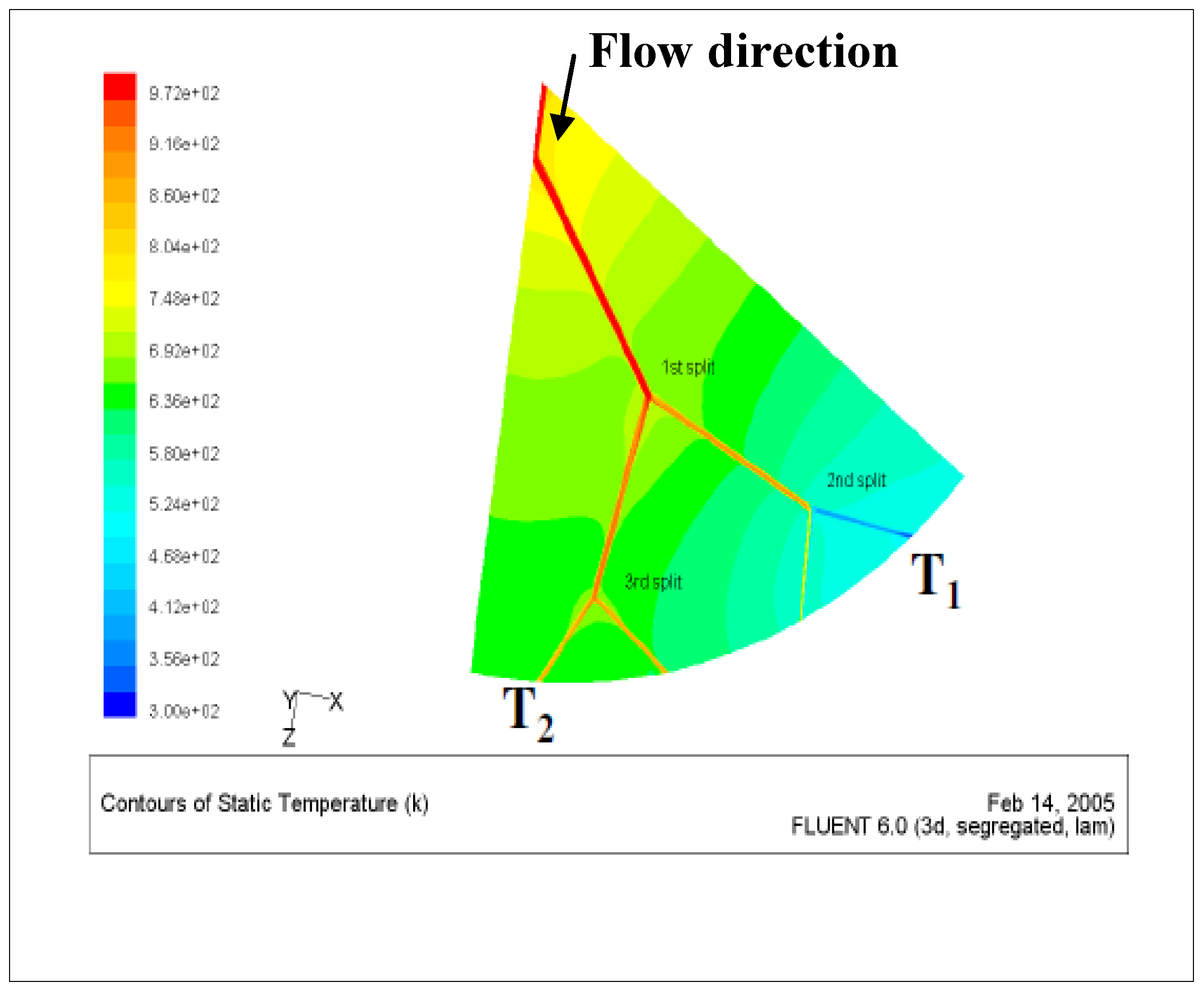
In natural flow systems (both inert and biological structures), why does a flow bifurcation (of the type shown in Figure 1) occur?

(b)

In man-made applications, is there an “optimal” bifurcation pattern for a given design goal, and how can it be identified?

Figure 1. The bifurcation geometry.

Figure 1. The bifurcation geometry.

A quantitative answer to the first question does not exist, and furthermore the problem involves such a large number of relevant parameters (initial conditions and stochastic noise thereof, degree on interaction with the surroundings, even randomly occurring external events) that a satisfactory predictive paradigm has not yet been proposed. Let us therefore focus our attention on the second question: the conventional approach followed by heat transfer practitioners is that of devising a set of similar (or modular) structures (each member being a properly constructed series of bifurcations) and to check a posteriori which member of the family attains the best performance under a pre-assigned set of design constraints. This heuristic approach may be very successful in practice [1,2,3], but its final result (the “optimal” structure) strongly and unavoidably depends on the initial choice of the geometrical features the “family” must possess: in other words, the final result essentially depends on the ingenuity and insight of the designer. An additional problem with this approach is that, once the “optimal” structure has been identified, every subsequent modification to its features may require a global iteration, i.e., a construction of a new family of structures each one of them possessing this “new” feature, and a new optimization. In other words, the optimum is not guaranteed to be global, when considered in the “attribute space” of the geometric or physical features of the set.

Given these premises, the starting point of the present analysis can only be very pragmatic and somewhat restricted in its breadth: when designing a bifurcation, can the designer (be it a human or nature itself) take entropy as the objective function of the optimisation? Limiting our discussion for the moment to anthropic structures, let us observe that for (laminar or turbulent) liquid flow in pipes, all current design manuals suggest to “minimize the pressure drop for a specified mass flowrate”, which is attained by limiting for instance sharply curved pipes, sudden restrictions or expansions, the interposition of diaphragms and valves, etc. But if the design goal is to carry a given mass flowrate m₀ from one “source” O to two delivery “sinks” A and B (Figure 1), can an “optimal” geometry be identified a priori?

The usual engineering qualification we assign to the concept of “optimal structure” would in this case apply to the flow path that, under the given design constraints, delivers the specified mass flowrate with the minimum possible irreversibility. This statement is a particular case of a much broader concept, namely that in the real world (in a more general perspective, “in nature”) the optimisation criterion is the minimum entropy generation rate compatible with the available exergy input and with the prescribed constraints.

Bifurcated flows are important per se, in piping for instance, but they are also interesting because they may be used as “building stones” to construct a porous matrix, or to reproduce, by successive splits and possibly by their recombination downstream, “fractal” geometries. A first goal of this study is to decide whether the optimal configuration exists, and if it exists whether the optimum is sharp and unique. The method falls under the class of “Entropy Generation Minimization” (formulated in its modern form by Bejan, [4]). In the laminar, isothermal and incompressible case analysed here, the only contribution to the entropy generation comes from the viscous dissipation, which is commonly measured by the pressure drop per unit length. The two “measures” (the pressure drop and the viscous entropy generation rate) may be numerically equivalent, in the sense that the minimum of the former coincides with the minimum of the latter, but the insight provided by an entropic analysis is much deeper, if only for the fact that it can be assessed locally [5,6] and immediately applied to design modifications.

Figure 2. The “bifurcated disc” studied in [5,7].

Figure 2. The “bifurcated disc” studied in [5,7].

2. The Entropy Generation Rate in a Channel

2.1. The standard derivation of the velocity profile in plane Poiseuille flow

It is useful to begin by examining the well-known textbook derivation of the plane Poiseuille flow that proceeds from a solution of the properly simplified Navier-Stokes equations. The physical assumptions are: steady, laminar, fully developed, isothermal flow of a Newtonian fluid with constant properties. The boundary conditions are: u = 0 at y = 0 and at y = d (wall b.c.). The solution is:

$$\text{u}=\frac{\Delta \text{p}{\text{d}}^2}{2\mathsf{\mu }\text{L}}\left(\frac{{\text{y}}^2}{{\text{d}}^2}-\frac{\text{y}}{\text{d}}\right)$$

(1)

From the velocity profile one can compute the local entropy generation:

$$\dot{\text{s}}(\text{y})=\frac{\mathsf{\mu }}{\text{T}}{\left(\frac{\text{du}}{\text{dy}}\right)}^2=\frac{{\text{d}}^2{\left(\Delta \text{p}\right)}^2}{\mathsf{\mu }{\text{L}}^2\text{T}}\left(\frac{{\text{y}}^2}{{\text{d}}^2}-\frac{\text{y}}{\text{d}}+\frac{1}{4}\right)$$

(2)

Since the pressure gradient is linked to the mass flow rate by:

$$\frac{\Delta \text{p}}{\text{L}}=\frac{12\mathsf{\nu }\dot{\text{m}}}{{\text{d}}^3}$$

(3)

The entropy generation in a channel of length L becomes (per unit channel width “z”):

$${\dot{\text{s}}}_{\text{L},\text{d}}=\frac{12\mathsf{\nu }{\dot{\text{m}}}^2\text{L}}{\mathsf{\rho }\text{T}{\text{d}}^4}={\text{K}}_{\mathrm{f}}\frac{{\dot{\text{m}}}^2\text{L}}{{\text{d}}^4}$$

(4)

From equation (4) we see that, as it was to be expected and it is confirmed by experiments, $\dot{\text{s}}$ grows with increasing channel length L and with decreasing channel width d.

2.2. Alternative derivation of the velocity profile of plane Poiseuille flow

For the following of this paper, it is interesting to examine a variational, and exact, alternative derivation of the Poiseuille velocity profile. For the steady, laminar, isothermal and fully developed flow considered in the previous Section, let us search for the velocity profile that minimises the viscous entropy generation in the fluid:

$${\dot{\text{s}}}_{\text{v}}=\frac{\mathsf{\mu }}{\text{T}}{\left(\frac{\text{du}}{\text{dy}}\right)}^2$$

(5)

The relevant variables in the optimisation are u, du/dx=0, du/dy. The Euler-Lagrange equations for this variation reduce to:

$$\left(\frac{\partial {\dot{\text{s}}}_{\text{v}}}{\partial \text{u}}\right)-\frac{\partial }{\partial \text{x}}\left[\frac{\partial {\dot{\text{s}}}_{\text{v}}}{\partial \left(\frac{\partial \text{u}}{\partial \text{x}}\right)}\right]-\frac{\partial }{\partial \text{y}}\left[\frac{\partial {\dot{\text{s}}}_{\text{v}}}{\partial \left(\frac{\partial \text{u}}{\partial \text{y}}\right)}\right]=...=\frac{2\mathsf{\mu }}{\text{T}}\frac{{\partial }^2\text{u}}{\partial {\text{y}}^2}$$

(6)

The boundary conditions on u and the additional constraint that the flow must transport a prescribed mass flow rate provide:

$$\text{u}=\frac{\Delta \text{p}{\text{d}}^2}{2\mathsf{\mu }\text{L}}\left(\frac{{\text{y}}^2}{{\text{d}}^2}-\frac{\text{y}}{\text{d}}\right)$$

(7)

i.e., the Poiseuille velocity profile. This result is indeed general [8]: for viscous, isothermal steady flow the Navier-Stokes equations admit of a variational formulation whose Lagrangian is the rate of exergy destruction (${\text{T}}_0\dot{\text{s}}$). There is no definitive proof yet that this is also the Lagrangian for thermal transport by convection, but it would seem reasonable to assume so [9,10,11,12].

The study presented in this paper was originated by the consideration that, if the entropy generation “governs” the structure of the flow in a channel, it could well be the “Lagrangian” for the structure of more complex flow domains.

In the following, the optimal bifurcation configuration is derived from a “constrained minimum realizable $\dot{\text{s}}$” principle.

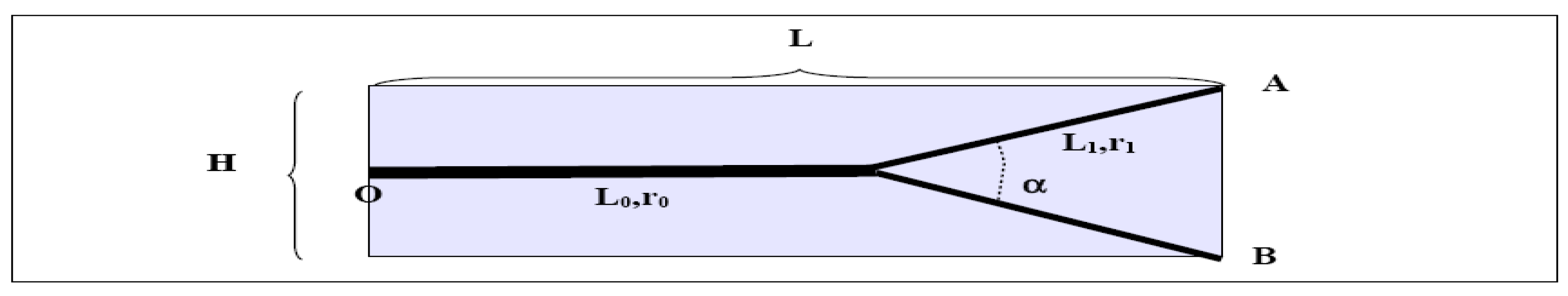
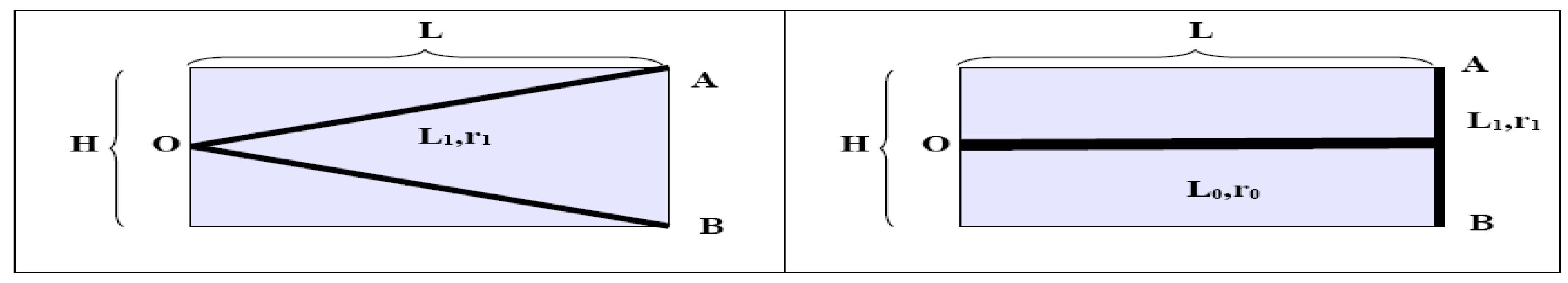
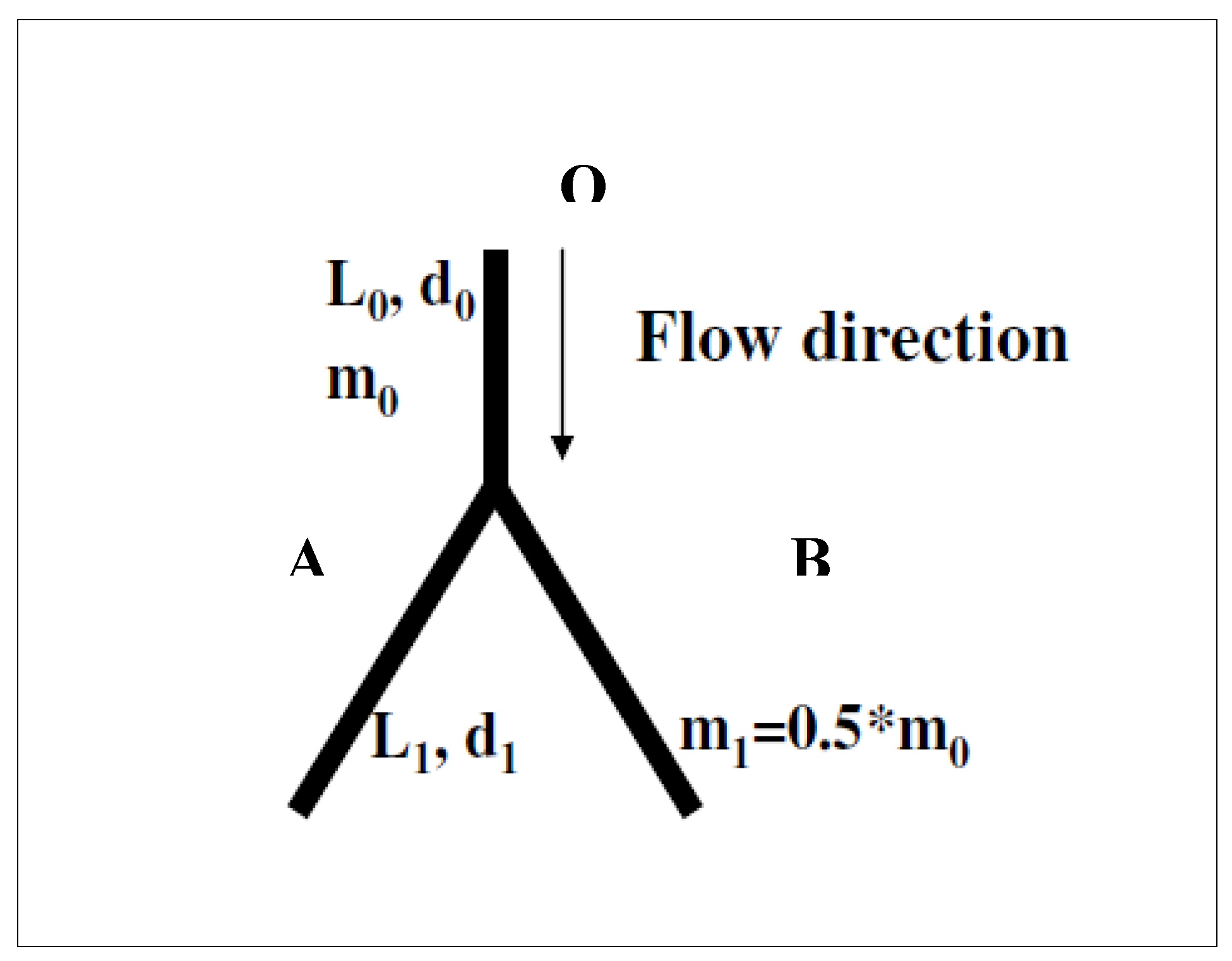
3. The Entropy Generation Rate in a Simple Bifurcation

Consider a rectangular element of a given aspect ratio a_r = H/L (Figure 3). In this simple model, the fluid proceeds from left to right, and the “goal” of the device is to deliver the mass flow rate m₀/2 to each one of the end points A and B. To provide a more realistic example, let us consider here that the channel is of circular section, so that instead of Equation (4) — the equivalent formulae for steady, laminar, fully developed flow in a round pipe apply.

Figure 3. Definition of the bifurcation geometry.

Figure 3. Definition of the bifurcation geometry.

The relevant variables are: m₀, m₁, L₀, L₁, d₀, d₁, and the (constant) fluid properties. The mass flow rate m₀ is prescribed, and the bifurcation is flow-wise symmetrical, so that m₁ = 0.5 m₀. The flow is isothermal.

Since the “goal” of the (natural or artificial) device is to deliver fluid to both endpoints A and B, a bifurcation must occur somewhere in the fluid path: let us examine first the two limit cases in which the fluid path splits at x = 0 (“V-flow”, Figure 4a) and at x = L (“T-flow”, Figure 4b).

Figure 4. The two limit cases: “V-flow” (a) and “T-flow” (b).

Figure 4. The two limit cases: “V-flow” (a) and “T-flow” (b).

The entropy generation rates are respectively:

$${\dot{\text{S}}}_{\text{V-flow}}=2{\dot{\text{S}}}_{{\text{L}}_1,{\text{r}}_1}={\text{K}}_{\text{f}}\frac{{\dot{\text{m}}}_0^2\text{L}}{{\text{r}}_0^4}\frac{\sqrt{1+0.25{\text{a}}_{\text{r}}^2}}{2{\mathsf{\delta }}^4}$$

(8a)

$${\dot{\text{S}}}_{\text{T-flow}}={\dot{\text{S}}}_{{\text{L}}_0,{\text{r}}_0}+2{\dot{\text{S}}}_{{\text{L}}_1,{\text{r}}_1}={\text{K}}_{\text{f}}\frac{{\dot{\text{m}}}_0^2\text{L}}{{\text{r}}_0^4}\left(1+\frac{{\text{a}}_{\text{r}}}{4{\mathsf{\delta }}^4}\right)$$

(8b)

With ${\text{K}}_{\text{f}}=\frac{8\mathsf{\nu }}{\mathsf{\pi }\mathsf{\rho }\text{T}}$ except for these two extreme cases, the bifurcation will take place somewhere in L, at a point P identified by an additional parameter λ = L₀/L; and the general expression for the entropy generation rate is:

$${\dot{\text{S}}}_{\text{bifurcated-flow}}={\dot{\text{S}}}_{{\text{L}}_0,{\text{r}}_0}+2{\dot{\text{S}}}_{{\text{L}}_1,{\text{r}}_1}={\text{K}}_{\text{f}}\frac{{\dot{\text{m}}}_0^2\text{L}}{{\text{r}}_0^4}\left[\mathsf{\lambda }+\frac{\sqrt{(1-{\mathsf{\lambda }}^2)+0.25{\text{a}}_{\mathrm{r}}^2}}{2{\mathsf{\delta }}^4}\right]$$

(9)

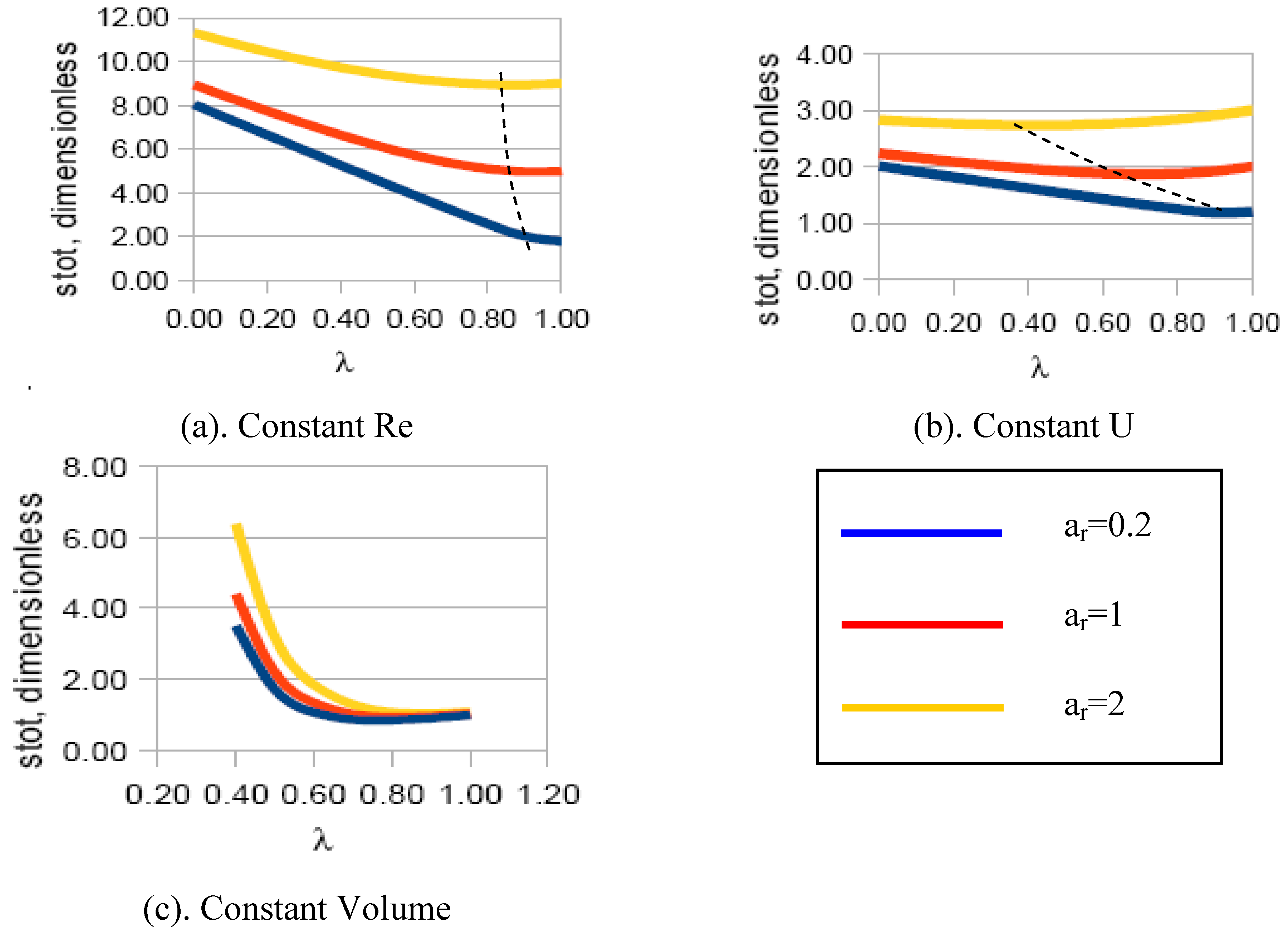
4. Results and Discussion

Equation (9) was solved analytically for different aspect ratios a_r = H/L and different bifurcation lengths (identified by the ratio λ = L₀/L), under three physically meaningful situations:

(1)

The Reynolds number remains constant over the entire fluid path: Re₀ = Re₁. This defines a diameter ratio δ = r₁/r₀ = 0.5;

(2)

The velocity remains constant over the entire fluid path: U₀ = U₁. This defines a diameter ratio δ = r₁/r₀ = 0.707;

(3)

The volume occupied by the fluid in the unsplit portion is equal to that occupied by the two bifurcated branches. This defines a diameter ratio δ = r₁/r₀ = $\sqrt{\frac{{\text{L}}_0}{2{\text{L}}_1}}$.

Notice that none of the above situations is per se “optimal” in any sense: they were selected because they provide a good spectrum for the actually possible (i.e., naturally occurring) configurations.

In Section 4.1, the results are presented for an ideal case, in which the entropy generation rate is given by Equation (9). In Section 4.2, the entropy generation rate is still given by Equation (9), but the losses due to the bifurcation are accounted for on the basis of an equivalent hydraulic length.

4.1. The ideal case, no bifurcation losses

The results for this case are shown in Figure 5a, b and c. The values of the entropy generation rates are made dimensionless by dividing them by the value:

$${\dot{\text{S}}}_{\text{ref}}={\mathrm{K}}_{\text{f}}\frac{{\dot{\text{m}}}_0^2\text{L}}{{\text{r}}_0^4}$$

(10)

(with the constant K_f defined in Section 3 above), that represents the viscous dissipation in a straight (i.e., unsplit) tube of length L and radius r₀. The following features are apparent:

(a)

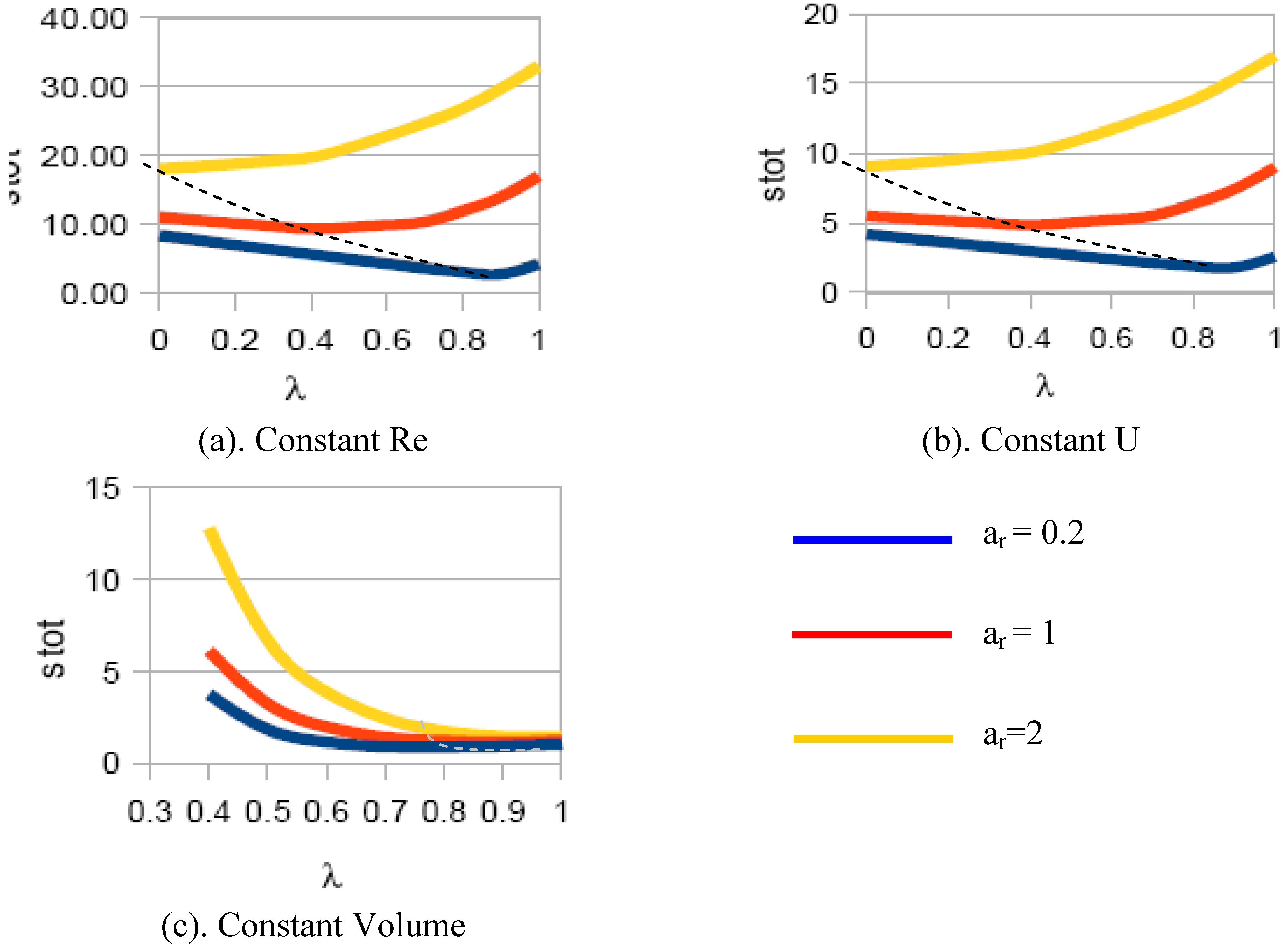
For all cases, the entropy generation rate strongly depends on the aspect ratio a_r of the domain in which the bifurcation occurs. With the geometry selected here, higher a_r lead — for the same splitting ratio λ — to a longer bifurcated stretch, of smaller diameter and therefore with higher losses;

(b)

The constant velocity case displays a lower entropy generation rate than the constant Re case for any bifurcation length. This is due to the fact that the mass conservation constraint imposes a higher diameter ratio on the split portions of the tubes that are therefore affected by a lower dissipation rate;

(c)

The constant fluid volume configurations display extremely high entropy generation rates for low splitting ratios, but are the least dissipative structure for high. However, the minimum dissipation is attained with diameter ratios near unity: the short bifurcations have a larger diameter than the initial portion of the channel, and the velocities are under the specified mass flow rate constraint correspondingly lower.

(d)

For each physical situation (constant Re, constant U, and constant V_fluid) there is indeed a rather well identifiable “optimal” configuration for each aspect ratio that displays a minimum value of the entropy generation rate. The exact values are reported in Table 1.

Figure 5. Dimensionless entropy generation in the bifurcation, without splitting losses. The dashed lines indicate the loci of the optimum.

Figure 5. Dimensionless entropy generation in the bifurcation, without splitting losses. The dashed lines indicate the loci of the optimum.

The above results are more general than those obtained by using allometric or arithmetic/geometrical laws. In fact, the latter models can be adjusted to obtain the same results as in the EGM method only after some non-trivial modification:

(1)

Use of an “optimal” diameter ratio (the basic assumption of all allometric models) is avoided, since this parameter is uniquely specified once the physical flow type has been assigned (constant Re, constant U, constant fluid volume);

(2)

A suitable physical correlation is introduced in the above mentioned models to link the “optimal” splitting ratio λ to the diameter ratio δ. in such a way that the minimum entropy generation — which is the most reasonable indicator of “optimal performance” — is at least one of the components of the objective function;

(3)

An additional correction is also introduced in the models to allow for the higher-than-unity diameter ratio δ. found for the “constant volume” configurations, which is a case not contemplated either by allometric [1,13,14] nor by arithmetic/geometrical (including fractal) [3,15] paradigms.

Table 1. Optimal splitting length ratio for minimum entropy generation, without splitting losses.

Case: Re0 = Re1	δ =r1/r0		Minimum $\frac{\dot{S}}{\dot{S_{ref}}}$
ar = 0.2	0.5	1	1.80
ar = 1	0.5	0.9	4.98
ar = 2	0.5	0.9	8.94
Case: U0 = U1	δ =r1/r0		Minimum $\frac{\dot{S}}{\dot{S_{ref}}}$
ar = 0.2	0.707	0.9	1.18
ar = 1	0.707	0.7	1.87
ar = 2	0.707	0.4	2.73
Case: V0 = 2V1	δ =r1/r0		Minimum $\frac{\dot{S}}{\dot{S_{ref}}}$
ar = 0.2	1.15	0.8	0.86
ar = 1	1.15	0.8	0.95
ar = 2	1.36	0.9	1.05

Table 1. Optimal splitting length ratio for minimum entropy generation, without splitting losses.

Case: Re0 = Re1	δ =r1/r0		Minimum $\frac{\dot{S}}{\dot{S_{ref}}}$
ar = 0.2	0.5	1	1.80
ar = 1	0.5	0.9	4.98
ar = 2	0.5	0.9	8.94
Case: U0 = U1	δ =r1/r0		Minimum $\frac{\dot{S}}{\dot{S_{ref}}}$
ar = 0.2	0.707	0.9	1.18
ar = 1	0.707	0.7	1.87
ar = 2	0.707	0.4	2.73
Case: V0 = 2V1	δ =r1/r0		Minimum $\frac{\dot{S}}{\dot{S_{ref}}}$
ar = 0.2	1.15	0.8	0.86
ar = 1	1.15	0.8	0.95
ar = 2	1.36	0.9	1.05

4.2. A more realistic case with added bifurcation losses

In real flows, an additional viscous dissipation is generated at the bifurcation, due to the stagnation flow at the cusp. These losses were demonstrated to be non-negligible in a previous numerical study [16], and are accounted for here in a much simplified manner, by introducing an “equivalent length” of tube on the bifurcated portion of the domain. Adopting this approximate method, the length L₁ in Equation (9) is multiplied by a factor (1 + n_D): the constant n_D can be derived from one of the many semi-empirical correlations for pressure losses in sudden restrictions, and the values assumed here are displayed in Figure 6. The results are shown in Figure 7a-c. The values of the entropy generation rates are made dimensionless like in the previous case.

Figure 6. The additional loss factor used to assess the viscous losses localized at the cusp.

Figure 6. The additional loss factor used to assess the viscous losses localized at the cusp.

Figure 7. Dimensionless entropy generation in the bifurcation, with splitting losses.

Figure 7. Dimensionless entropy generation in the bifurcation, with splitting losses.

With respect to the previous “ideal” case, the following additional features emerge:

(a)

For all cases, the entropy generation rate displays a marked increase: for the same aspect ratio a_r, same splitting length and same diameter ratio, the dissipation is increased of a factor between 1.5 and 4. This confirms the importance of real-flow effects on the optimal configuration;

(b)

For each physical situation (constant Re, constant U, constant V_fluid) there is still an “optimal” configuration that displays a minimum value of the entropy generation rate, but the minimum is markedly shifted towards lower splitting ratios (earlier bifurcation), except for the constant volume case, in which it is very near the “T” configuration (λ≈1). The exact values are reported in Table 2.

Table 2. “Optimal” splitting length ratio λ for minimum entropy generation, with splitting losses.

Case: Re0 = Re1	δ = r1/r0	λ	Minimum $\frac{\dot{S}}{\dot{S_{ref}}}$
ar = 0.2	0.5	0.9	2.71
ar = 1	0.5	0.4	9.81
ar = 2	0.5	0	18.07
Case: U0 = U1	δ = r1/r0	λ	Minimum $\frac{\dot{S}}{\dot{S_{ref}}}$
ar = 0.2	0.707	0.9	1.80
ar = 1	0.707	0.4	4.85
ar = 2	0.707	0	9.03
Case: V0 = 2V1	δ = r1/r0	λ	Minimum $\frac{\dot{S}}{\dot{S_{ref}}}$
ar = 0.2	1.15	0.8	0.88
ar = 1	1.36	0.9	1.14
ar = 2	1.50	1	1.40

Table 2. “Optimal” splitting length ratio λ for minimum entropy generation, with splitting losses.

Case: Re0 = Re1	δ = r1/r0	λ	Minimum $\frac{\dot{S}}{\dot{S_{ref}}}$
ar = 0.2	0.5	0.9	2.71
ar = 1	0.5	0.4	9.81
ar = 2	0.5	0	18.07
Case: U0 = U1	δ = r1/r0	λ	Minimum $\frac{\dot{S}}{\dot{S_{ref}}}$
ar = 0.2	0.707	0.9	1.80
ar = 1	0.707	0.4	4.85
ar = 2	0.707	0	9.03
Case: V0 = 2V1	δ = r1/r0	λ	Minimum $\frac{\dot{S}}{\dot{S_{ref}}}$
ar = 0.2	1.15	0.8	0.88
ar = 1	1.36	0.9	1.14
ar = 2	1.50	1	1.40

As in the previous case, and for the same reasons, the above results are incompatible with allometric and geometric/fractal paradigms.

5. Conclusions

The study reported here is performed under a strongly idealized set of assumptions that may limit its validity in practical applications: in practice, what has been discussed in this paper is a metaphor rather than a design paradigm. It is clear that an experimental or numerical validation of the results obtained here is in order. However, even at the present level of an analytical analysis of a strongly simplified model, the general trends displayed by the solution are very relevant, and can be summarized as follows:

(a)

For all examined situations, a configuration exists that displays the lowest viscous entropy generation rate compatible with the imposed constraints;

(b)

In all cases, the diameter ratio δ can be derived from purely phenomenological considerations: there is no a priori optimal value for this parameter;

(c)

The entropy generation rate appears to be a consistent Lagrangian for the identification of the “optimal” configuration, and furthermore, the optima thus derived appear different from those suggested by both allometric and arithmetic/geometric models.

A general, very widely published theory exists (Constructal Theory, formulated by Bejan [17,18,19,20]) that attempts to explain and interpret the geometry of material and immaterial flows without recurring to any explicit “optimization method” or any “objective function”. Though it is very likely that a structural relationship exists between Constructalism and Entropy Generation Minimization (see also [18,21]), the problem has not yet been analyzed in its entirety, especially in view of the generally accepted a posteriori paradigm that “more efficient” flows display “minimal” entropy generation rates (quotation marks are used to stress the approximate meaning of both quantifiers). This preliminary study demonstrates — on the basis of simple analytical considerations — that the entropy generation rate is indeed a proper quantifier for the bifurcation topology, in the sense that it identifies the shape that, for each set of assigned boundary conditions, performs the assigned task (to deliver a given mass flow rate) with the minimal exergy destruction (irreversible entropy generation rate).

It is important to stress that the procedure adopted in the present study is perfectly falsifiable: if a minimum entropy generation rate configuration can be demonstrated to exist outside of the ranges identified by the method presented here, then the method is incorrect and needs to be revised (it has been “falsified”). This feature suggests a verification procedure: generate — numerically or experimentally — a sufficiently extensive series of bifurcated configurations, and identify the “least dissipative” ones. A multi-variable fit of the generated solutions may then be used to heuristically determine the underlying Lagrangian.

References

1. Cano-Andrade, S.; Hernandez-Guerrero, A.; von Spakovsky, M.R.; Damian-Ascencio, C.E.; Rubio-Arana, J.C. Current density and polarization curves for radial flow field patterns applied to PEMFCs. Energy 2010, in press. [Google Scholar] [CrossRef]
2. Escher, W.; Michel, B.; Poulikakos, D. Efficiency of optimized bifurcating tree-like and parallel microchannel networks in the cooling of electronics. Int. J. Heat Mass Transfer 2008, 07, 48. [Google Scholar] [CrossRef]
3. Ramos-Alvarado, B.; Hernandez-Guerrero, A.; Juarez-Robles, D.; Li, P.; Rubio-Arana, J.C. Parametric study of a symmetric flow distributor. In Proceedings of ASME-IMECE, Lake Buena Vista, FL, USA, November 2009.
4. Bejan, A. Entropy Generation Minimization; CRC Press: New York, NY, USA, 1995. [Google Scholar]
5. Robbe, M.; Sciubba, E. A 2-D constructal configuration genetic optimization method. In Proceeding of ASME-IMECE, Boston, MA, USA, May 2008.
6. Robbe, M.; Sciubba, E. Derivation of the optimal internal cooling geometry of a prismatic slab: Comparison of constructal and non-constructal geometries. Energy 2009, 34, 2167–2174. [Google Scholar] [CrossRef]
7. Robbe, M.; Sciubba, E.; Bejan, A.; Lorente, S. Numerical analysis of a tree-shaped cooling structure for a 2-D slab: A validation of a “constructally optimal” configuration. In Proceedings of VIII ESDA-ASME Conference, Torino, Italy, July 2006.
8. Sciubba, E. Do the Navier-Stokes equations admit a variational formulation? In Variational and Extremum Principles in Macroscopic Systems; Sieniutycz, S., Farkas, H., Eds.; Elsevier: Oxford, UK, 2004. [Google Scholar]
9. Geskin, E.S. A variational principle for transport processes in continuous systems: Derivation and application. In Variational and Extremum Principles in Macroscopic Systems; Sieniutycz, S., Farkas, H., Eds.; Elsevier: Oxford, UK, 2004. [Google Scholar]
10. Glansdorff, P.; Prigogine, I. On a general evolution criterion in macroscopic physics. Physica 1964, 30, 351–374. [Google Scholar] [CrossRef]
11. Gyarmati, I. Non-Equilibrium Thermodynamics; Springer-Verlag: Berlin, Germany, 1970. [Google Scholar]
12. Sieniutycz, S. Field variational principles for irreversible energy and mass transfer. In Variational and Extremum Principles in Macroscopic Systems; Sieniutycz, S., Farkas, H., Eds.; Elsevier: Oxford, UK, 2004. [Google Scholar]
13. Hess, W.R. Das Prinzip des kleinsten Kraftverbrauches im Dienste hämodynamischer Forschung. Arch. Anat. Physiol. (Physiol. Abteil.) 1914, 1/2, 1–62. [Google Scholar]
14. Murray, C.D. The physiological principle of minimum work: I. The vascular system and the cost of blood. Natl. Acad. Sci. 1926, 12, 207–214. [Google Scholar] [CrossRef]
15. Rubio-Jimenez, C.A.; Hernandez-Guerrero, A.; Rubio-Arana, J.C.; Kandlinkar, S. Natural patterns applied to the design of microchannel heat sinks. In Proceedings of ASME-IMECE, Lake Buena Vista, Florida, USA, November 2009.
16. Robbe, M. CFD Analysis of the Thermo-Fluidynamic Performance of Constructal Structures. Ph.D. Thesis, University of Roma 1, Rome, Italy, 2007. [Google Scholar]
17. Bejan, A. Constructal-theory network of conducting paths for cooling a heat generating volume. Int. J. Heat Mass Transfer 1997, 40, 799–816. [Google Scholar] [CrossRef]
18. Bejan, A. Shape and Structure from Engineering to Nature; Cambridge U. Press: Cambridge, UK, 2000. [Google Scholar]
19. Bejan, A.; Rocha, L.A.O.; Lorente, S. Thermodynamic optimization of geometry: T- and Y-shaped constructs of fluids streams. Int. J. Therm. Sci. 2000, 39, 946–960. [Google Scholar] [CrossRef]
20. Bejan, A.; Lorente, S. The constructal law and the thermodynamics of flow systems with configuration. Int. J. Heat Mass Transfer 2004, 47, 3203–3214. [Google Scholar] [CrossRef]
21. Sciubba, E. Constructal theory & variational principles for the Navier-Stokes equations: Is there a link? In Proceedings of Workshop on Constructal Theory of the Generation of Optimal Flow Configuration, Rome, Italy, March 2005.