Article

Wavelet-Based Analysis on the Complexity of Hydrologic Series Data under Multi-Temporal Scales

1
State Key Laboratory of Pollution Control and Resource Reuse, Department of Hydrosciences, School of Earth Sciences and Engineering, Nanjing University, Nanjing 210093, China
2
China Water International Engineering Consulting Co. Ltd., Beijing 100053, China
3
Hydrology Bureau of Yellow River Conservancy Committee of Ministry of Water Resources, Zhengzhou 450001, China
*
Author to whom correspondence should be addressed.
Entropy 2011, 13(1), 195-210; https://doi.org/10.3390/e13010195
Submission received: 1 December 2010 / Revised: 21 December 2010 / Accepted: 22 December 2010 / Published: 17 January 2011

Abstract

:
In this paper, the influence of four key issues on wavelet-based analysis of hydrologic series’ complexity under multi-temporal scales, including the choice of mother wavelet, noise, estimation of probability density function and trend of series data, was first studied. Then, the complexities of several representative hydrologic series data were quantified and described, based on which the performances of four wavelet-based entropy measures used commonly, namely continuous wavelet entropy (CWE), continuous wavelet relative entropy (CWRE), discrete wavelet entropy (DWE) and discrete wavelet relative entropy (DWRE) respectively, were compared and discussed. Finally, according to the analytic results of various examples, some understanding and conclusions about the calculation of wavelet-based entropy values gained in this study have been summarized, and the corresponding suggestions have also been proposed, based on which the analytic results of complexity of hydrologic series data can be improved.

1. Introduction

Hydrologic processes in nature are influenced by many and often associated physical factors, mainly involving the climatic and land surface conditions [1,2,3]. Moreover, when encountering the great influence of climatic change [4,5] and human activities [6,7], hydrologic time series show more complicated characteristics. Observed hydrologic series usually show non-stationary and multi-temporal scale characteristics in daily, monthly, annual and multi-annual processes [3,8]. Revelation of these complicated characteristics, as well as description of hydrologic series’ complexity, is a substantial issue in the field of stochastic hydrology, because it is not only the basis of hydrologic forecasting, water resources management and many other practical water activities, but also the basis of evaluating the impacts of climatic change and human activities on hydrologic processes [9].
Presently information theories have been widely applied in hydrology to quantify the variability in hydrologic variables (e.g., precipitation, runoff, temperature and discharge) [10,11,12], in which the Shannon entropy is a primary measure of the degree of uncertainty, such as disorderliness, randomness and irregularity [13,14]. Generally, higher entropy reflects more random and complicated systems, and vice versa. Therefore, the highest entropy is assigned to white noise process that is completely random and unpredictable [9]. Presently, various entropy-based methods have been applied in hydrologic series analysis, such as the use of principle of maximum entropy (POME) in hydrologic frequency analysis [3,15], maximum entropy spectral analysis (MESA) in period identification [16]. As for the description of hydrologic series’ complexity, traditional entropy measures usually provide inaccurate or incomplete descriptions of hydrologic systems which generally operate over multi-temporal scales and have higher complexity than those just on a single scale [9,11]. Compared with traditional entropy measures, the sample entropy (SE) and multi-scale entropy (MSE) are more effective and applicable for analysis of those systems with multi-temporal scales characteristics [9,17,18], but they cannot deal with the non-stationary characteristics of hydrologic series data; moreover, many key parameters which are difficult to be accurately estimated in practice, such as the tolerance criterion and embedding dimension, influence their analytic results.
Another popular and powerful method of time series analysis is the wavelet analysis (WA) which presently has been widely applied to many fields of hydrology, because it has the advantage of elucidating localized characteristics of non-stationary time series both in temporal and frequency domains [19,20]. The wavelet entropy (WE), which is the combination of WA with information theory, is an important and commonly used concept of describing the complexity of hydrologic series under multi-temporal scales [21,22]. Concretely, it is used first to analyze hydrologic series data by WA, such as the continuous wavelet transform (CWT) and multi-resolution analysis (MRA), and then to calculate the entropy measures, mainly including the conventional Shannon entropy [13], mutual information content [23] and relative entropy [24]. However, when applying these wavelet-based entropy measures to hydrologic series, the analytic results are usually influenced by many key issues, such as the choice of mother wavelet, noise, estimation of probability density function (pdf), and series’ trend. To the authors’ knowledge, there are few studies on these key issues in present contributions, therefore the accuracy and reliability of analytic results of WE cannot be verified; moreover, the differences of performances of various wavelet-based entropy measures are also unknown.
Therefore, two main objectives are pursued in this study; one is to evaluate the influence of several key issues on the calculation of entropy values; and the other is to compare the performances of various wavelet-based entropy measures. To achieve the two goals, the wavelet theory and entropy measures used in this paper are briefly introduced in Section 2. In Section 3, the selected representative hydrologic series data are first described; then, the complexities of them are described by using various wavelet-based entropy measures, and analytic results are compared and discussed, based on which some understanding and findings are gained. Finally, this study is summarized and concluded in the last section.

2. Methods

2.1. Wavelet Analysis

We use wavelet analysis (WA) to reveal the multi-temporal scale characteristics of hydrologic series. The continuous wavelet transform (CWT) is operated via the translation and dilation (or contraction) of a mother wavelet ψ(t) across the series f(t) as a function of time t [8]:
W f ( a , b ) = + f ( t ) ψ a , b * ( t ) d t    with    ψ a , b ( t ) = | a | 1 / 2 ψ ( t - b a )    a , b R , a 0
where parameter a and b is temporal scale (TS) factor and time translation factor, respectively. ψ*(t) is the complex conjugate, and Wf(a,b) are continuous wavelet coefficients. On the basis of CWT results, the global wavelet spectrum (GWS) can be calculated, which presents the energy distribution of time series f(t) under multi-temporal scales:
G W S f ( a ) = 1 n ( W f ( a , b ) ) 2 d b
where n is series’ length. In nature, observed hydrologic series are more often discrete signals, so the parameter a and b are discretized, and then the discrete wavelet transform (DWT) is operated as:
W f ( j , k ) = + f ( t ) ψ j , k * ( t ) d t    with    ψ j , k ( t ) = a 0 j / 2 ψ ( a 0 j t b 0 k )    j , k Z , j 0
in which parameter a0 and b0 are constants; j and k are decomposition level (DL) and time translation factor respectively. In practice, the dyadic DWT is used commonly by setting a0 = 2, b0 = 1:
W f ( j , k ) = + f ( t ) ψ j , k * ( t ) d t    with    ψ j , k ( t ) = 2 j / 2 ψ ( 2 j t k )    j , k Z , j 0
The choice of mother wavelet and DL are two key issues in dyadic DWT. According to the theory of dyadic DWT [25], the theoretical maximum M of DL can be calculated by using Equation (5):
M = [ log 2 ( n f ( t ) ) ]
where [∙] means taking the integer part of real value in square bracket. nf(t) is the length n of series f(t).
If the wavelet used meets the “regularity” condition, the original signal, as well as its sub-signals under different DLs, can be reconstructed by using wavelet coefficients:
f ( t ) = k j W f ( j , k ) ψ j , k ( t )
Therefore, the time series f(t) after wavelet decomposition can be described as:
f ( t ) = f ¯ + j = 1 M f j ( t )
where f ¯ is the residual component reconstructed by using approximations wavelet coefficients under the DL M, which generally corresponds to the mean or trend of f(t). fj(t) is the sub-signal under the DL j reconstructed by using details wavelet coefficients [25].

2.2. Entropy Measures

We use two entropy measures, Shannon entropy and relative entropy, to quantify the complexity of hydrologic series in this paper. Their calculation methods are described as follows.
According to information theory [13], the Shannon entropy (H) is calculated as:
H ( x ) = i = 1 n p ( x i ) log 2 ( p ( x i ) )
where p(xi) is the pdf used to describe the random characters of variable x with the length of n. In Equation (8) the base of 2 is used, thus entropy is measured in bits. H is a measure of information; more information results in lower entropy, and vice versa. Therefore bigger value of H presents more disordered and complicated hydrologic systems.
Besides, relative entropy (RE) is a measure of the similarity between two variables x and y given by the pdf of p and q respectively, and it is described as:
R E ( x , y ) = i p i log 2 ( p i / q i )
Equation (9) can be interpreted as the amount of additional information necessary to represent p given the q. Therefore a smaller value of RE reflects better agreement between p and q [11]. The RE is used in this paper mainly to analyze the similarity between original series and its sub-signals under different TSs (or DLs), based on which we can identify the real components of series data.
Because the values of H and RE are calculated based on the wavelet results in this paper, four wavelet-based entropy measures are considered, namely continuous wavelet entropy (CWE), discrete wavelet entropy (DWE), continuous wavelet relative entropy (CWRE) and discrete wavelet relative entropy (DWRE) respectively. Furthermore, two approaches are used to estimate the pdf; one is the interval-sampling based on the assumption of series’ random characters [11], and the other is based on the wavelet energy distribution of series data [22]; they are called the Type-I pdf and Type-II pdf respectively for easily stating contents. The latter is described as follows.
The CWT-based pdf pE(a,b) is defined in Equation (10), and it is estimated according to the wavelet energy (i.e., variance):
p E ( a , b ) = E ( a , b ) E ( a ) = | W f ( a , b ) | 2 | W f ( a , b ) | 2 d b
in which E(a,b) presents the wavelet energy under TS a and time position b, whereas E(a) presents the total energy of series under TS a. The estimated pdf pE(a,b) of variables is substituted into Equation (8) and Equation (9) to calculate the CWE and CWRE respectively. Correspondingly, the DWT-based pdf pE(j,k) is defined as:
p E ( j , k ) = E ( j , k ) E ( j ) = W f ( j , k ) 2 k ( W f ( j , k ) ) 2
where E(j) presents the total energy of series under DL j. The estimated pdf pE(j,k) of variables is substituted into Equation (8) and Equation (9) to calculate the DWE and DWRE respectively.

3. Results and Discussion
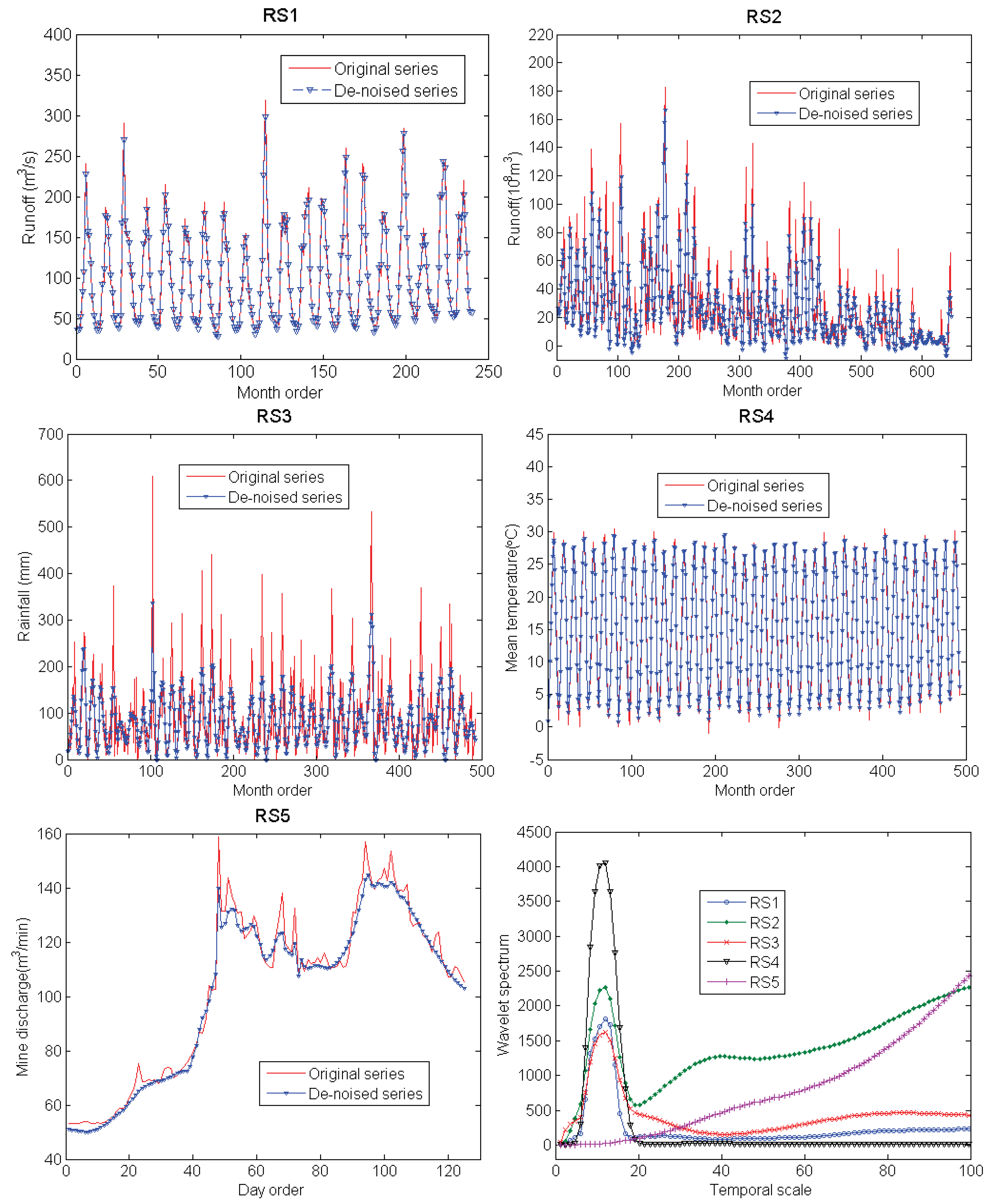
3.1. Data

We select five representative series of observed hydrologic data from various basins with obviously different climatic conditions, mainly to explain the relevant contents and to verify the conclusions in this paper. They are briefly described in Table 1, and their global wavelet spectra are presented in Figure 1.
Table 1. Five observed hydrologic series data used in this paper.
TypeAbbreviationLengthMeasured PlaceClimatic Condition
RunoffRS1276 months (1978–2000)Dashankou in the northwest of ChinaInland climate
RunoffRS2648 months (1950–2003)Lijin in the north of ChinaTemperate east-Asian monsoon climate
PrecipitationRS3492 months (1961–2001)Nanjing in the mid-east of Chinasubtropical monsoon climate
TemperatureRS4492 months (1961–2001)Nanjing in the mid-east of Chinasubtropical monsoon climate
Mine dischargeRS5125 days (June 1 to October 3 in 2003)Hanqiao in the mid-east of Chinasubtropical monsoon climate
Among them, the RS1, RS3 and RS4 series have a dominant period of 12 months; the RS2 series has a dominant period of 12 months and an obviously decreasing tendency; whereas the RS5 series has first an increasing and then a decreasing tendency, but no period. Moreover, their statistical characters, including mean ( x ¯ ), coefficient of variation (Cv), coefficient of skewness (Cs) and lag-1 autocorrelation coefficient (R1), are calculated and summarized in Table 2. The variability of RS2 series is the most obvious because the value of its Cv is 1.08, but the value of Cv of RS5 series is just as little as 0.30; the skew degree of RS3 series is the most obvious with the Cs value of 2.21, whereas the Cs of RS4 series has the smallest value of −0.07; the RS5 series has the best auto-correlate characteristics because its R1 is 0.96, but the R1 of RS3 series has the smallest value of 0.29.
Figure 1. De-noising results of five observed hydrologic series obtained by using the chosen wavelets, and the global wavelet spectra of them.
Entropy 13 00195 g001
To continue, we choose appropriate mother wavelets by using the method proposed in [26], and then remove noise in these series data by using the wavelet threshold de-noising (WTD) method proposed in [26,27], which is more effective than other traditional de-noising methods as discussed in [26,28,29]. The chosen wavelets are listed in Table 2, and the de-noising results are depicted in Figure 1. Calculation results of signal-to-noise ratio (SNR) indicate that RS4 series includes the smallest content of noise because its SNR value is 42.02, but the noise-contaminated degree of RS3 series is the worst with the SNR value of −0.59.
Table 2. Statistical characters of five observed hydrologic series used in this paper.
SeriesStatistical Characters*SNRWavelet Used
x ¯ CvCsR1
RS1107.460.631.290.7526.77dmey
RS227.051.081.910.7414.80coif4
RS386.950.932.210.29−0.59db10
RS415.450.59−0.070.8542.02db10
RS5103.500.30−0.320.9632.84sym5
* The statistical characters include mean ( x ¯ ), coefficient of variation (Cv), coefficient of skewness (Cs) and lag-1 autocorrelation coefficient (R1).
In the following four sub-sections, we mainly discuss the influence of four key issues, namely choice of wavelet, noise, estimation of pdf and series’ trends, on the calculation of wavelet-based entropy values. In the final sub-section, we compare the performances of four entropy measures, namely CWE, CWRE, DWE and DWRE. In the analytic process in each sub-section, we select two representative series data from Table 1 as examples, but do not analyze all series to save space.

3.2. Analysis of Influence of Wavelets

We use the RS1 and RS2 series as examples, which are little and greatly impacted by human activities, respectively, to discuss the influence of wavelets used on the calculation of wavelet-based entropy values. Specifically, we first choose various wavelets from different wavelet series whose mathematical properties can be found in [25], and then apply CWT to the two series data; finally we calculate the values of CWE and CWRE. The results are presented in Figure 2, based on which we compare the chosen wavelets in Table 2 with other wavelets. It indicates that analytic results of certain series under the whole temporal scales vary with the wavelets used, and four entropy values reflect obviously different complexities of series data. As a whole, the analytic results of RS1 and RS2 series obtained by using the chosen “dmey” and “coif4” wavelets in Table 2 are comparatively the best. As shown in Figure 2, the RS1 series has the dominant period of 12 months, and the value of its CWRE under the TS 12 but not other temporal scales obtained by using “dmey” is much close to zero; the RS2 series has the dominant period of 12 months and an obviously decreasing tendency, and the values of its CWRE under the TS 12 and big temporal scales obtained by using “coif4” are the most close to zero. Besides, it shows that the RS2 series as a whole is more complicated than RS1 series; this is due to the great influence of human activities on the Yellow River [30].
According to the wavelet theory, it is very easily understandable that because the choice of mother wavelet is the foremost task in all wavelet-based analytic processes [20,31], it also influences the calculation of wavelet-based entropy values. Therefore, this issue should be first considered and solved in the analysis of hydrologic series’ complexity. In this paper, the authors recommend the method proposed in [26], because its basic idea is to choose wavelet based on wavelets’ prosperities and analyzed series itself, which can make the chosen wavelet more reasonable. Besides, analytic results of RS1 and RS2 series in Figure 2 also verify the effectiveness of this method.
Figure 2. Calculation results of wavelet-based entropy values (CWE and CWRE) used to describe the complexities of RS1 and RS2 series using various wavelets.
Entropy 13 00195 g002

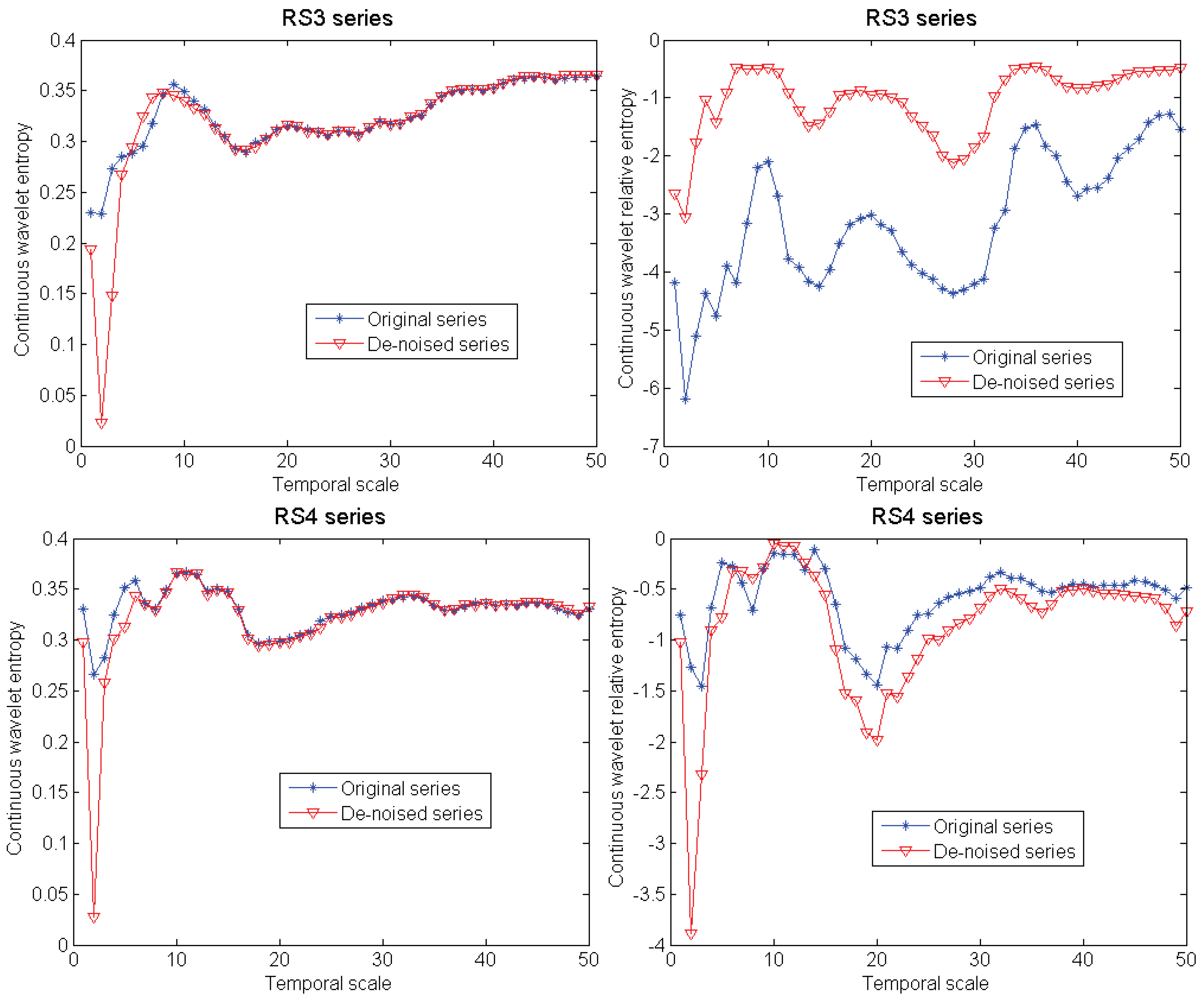
3.3. Analysis of Influence of Noise

We use the RS3 and RS4 series as examples, whose noise-contamination degrees are the worst and least respectively, to discuss the influence of noise on the calculation of wavelet-based entropy values. Concretely, we first remove noise in the two series data by WTD method; then, we apply CWT to both the original and de-noised series using the chosen “db10” wavelet in Table 2, and calculate the values of their CWE and CWRE finally.
Figure 3. Calculation results of wavelet-based entropy values (CWE and CWRE) used to describe the complexities of original and de-noised RS3 and RS4 series.
Entropy 13 00195 g003
The analytic results are depicted in Figure 3. It shows that the entropy values of original and de-noised series data show obvious differences, especially the results of the RS3 series with the SNR value of −0.59. As for the RS3 series, it includes too much noise, thus the values of CWRE of the de-noised series under the whole temporal scales are smaller than those of original RS3 series; as for the RS4 series, it has big SNR value of 42.02 and shows analogously trigonometric fluctuation with the period of 12 months, thus the entropy values (both CWE and CWRE) of the original and de-noised RS4 series under the whole temporal scales are similar to each other. Therefore, it can be concluded that noise has great influence on the complexity of hydrologic series data, that is, noise adds complexity to hydrologic series data, and the influence of noise becomes worse along with the decreasing value of SNR; moreover, noise has a more severe influence on the analytic results of CWRE than those of CEW. Besides, because the energy of noise mainly concentrates in small temporal scales, it has severer influence on the entropy values under small temporal scales than those under big temporal scales.
To sum up, noise has great influence on various processes of hydrologic series analysis [3,32,33,34,35], such as the periods’ identification, parameters estimation and hydrologic series prediction, and the calculation of entropy values is not a exception as discussed above. Here, the authors suggest the wavelet threshold de-noising method proposed in [26,27] be used in practice, because by using it not only the appropriate mother wavelet can be chosen, but also reliable de-noising results of hydrologic series data can correspondingly be obtained, based on which the analytic results of complexity of hydrologic series data can be improved.

3.4. Analysis of Influence of pdf

We use the RS1 and RS4 series as examples, both of which have a dominant period of 12 months, to discuss the influence of pdf estimated on the calculation of wavelet-based entropy values. Here, the two types of Type-I pdf and Type-II pdf are used. To be specific, we first remove noise in the RS1 and RS4 series, and then apply CWT to the two de-noised series; finally we calculate their CWE and CWRE using two different types of pdf. The analytic results are depicted in Figure 4. It shows that both the values of CWE and CWRE of series data show obvious differences when using different types of pdf. As a whole, the two curves of CWE obtained by using the two types of pdf have the same tendency; but the two CWRE curves are approximately inverse. Because the RS1 and RS4 series have a dominant period of 12 months, their CWRE values under TS 12 should be much closer to zero. However, Figure 4 indicates that the results obtained by using the Type-II pdf accord with this requirement, but those by using the Type-I pdf disobey this requirement.
Figure 4. Calculation results of wavelet-based entropy values (CWE and CWRE) used to describe the complexities of de-noised RS1 and RS4 series by using two types of pdf.
Entropy 13 00195 g004
Therefore, it can be held that the Type-II pdf is more effective and reasonable than Type-I pdf. In the authors’ opinion, this conclusion makes sense from the physical point of view. Because the Type-II pdf is estimated based on the energy distribution (both the characteristics and composition) of series data [22], by using it the complexity of hydrologic series data under multi-temporal scales can be quantified more accurately and reliably.

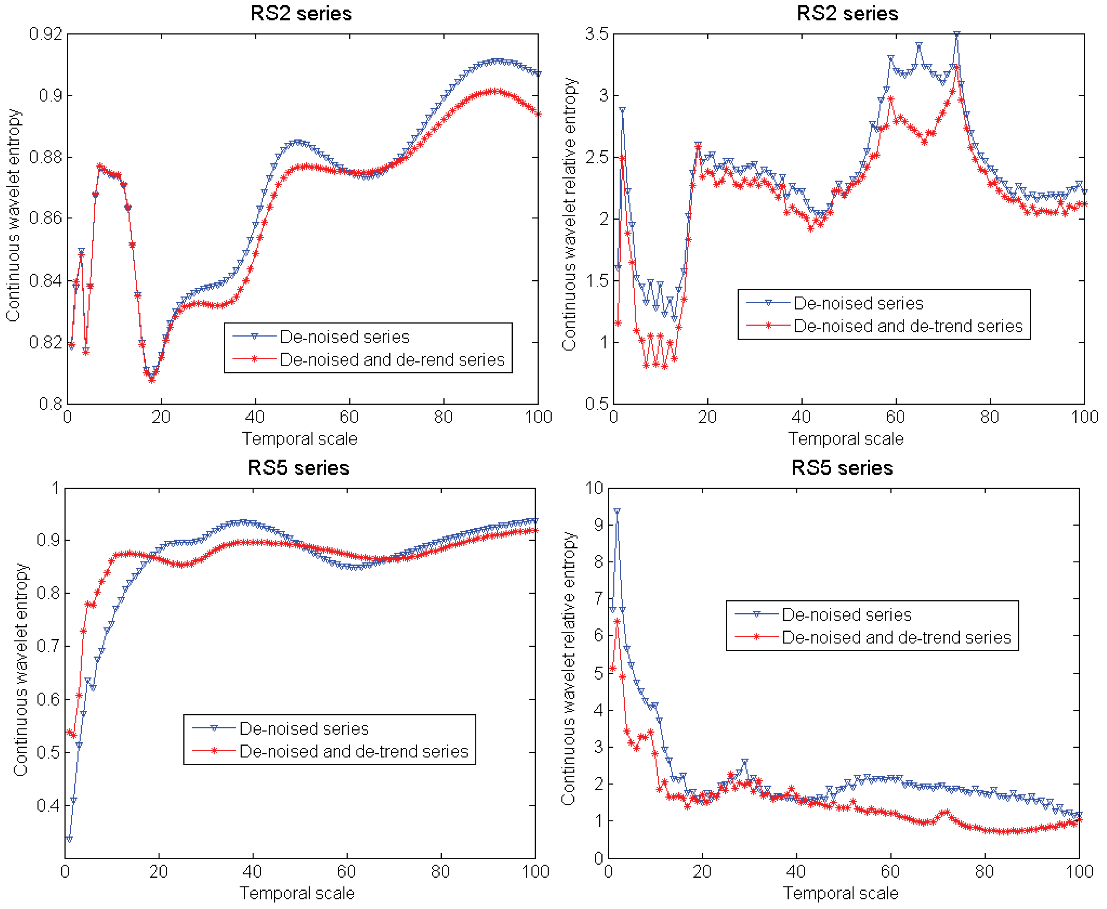
3.5. Analysis of Influence of Series’ Trend

Present studies demonstrate that if a trend is present in the series data analyzed, this will most likely cause the Type-I pdf to appear as a more uniform distribution, and will further result in increasing entropy values [11]. Considering that the Type-II pdf is more effective and reasonable than the Type-I pdf, as explained in the above sub-section, we here use the RS2 and RS5 series as examples, which have obviously decreasing and increasing-decreasing tendencies, respectively, mainly to discuss the influence of series’ trend on the calculation of wavelet-based entropy values when using the Type-II pdf.
Figure 5. Calculation results of wavelet-based entropy values (CWE and CWRE) used to describe the complexities of de-noised, and de-noised and de-trend RS2 and RS5 series.
Entropy 13 00195 g005
Specifically, we first remove trends of the two de-noised series data by subtracting their residual component f ¯ according to Equation (7), and then apply CWT to both the de-noised series, and the de-noised and de-trend series; finally we calculate their CWE and CWRE by using the Type-II pdf. The analytic results are presented in Figure 5. It indicates that series’ trend influences the calculation results of entropy values under big but not small temporal scales; moreover, the influence on CWRE is severer than that on CWE. Generally speaking, series’ trends cause increasing values of entropy; for example, the values of CWRE of de-noised RS5 series under the temporal scales of 60–80 are bigger than 2, but those of the de-noised and de-trend RS5 series under the temporal scales of 60–80 are smaller than 1. Therefore, the trend of series data should get more attention in the analytic process of hydrologic series’ complexity.

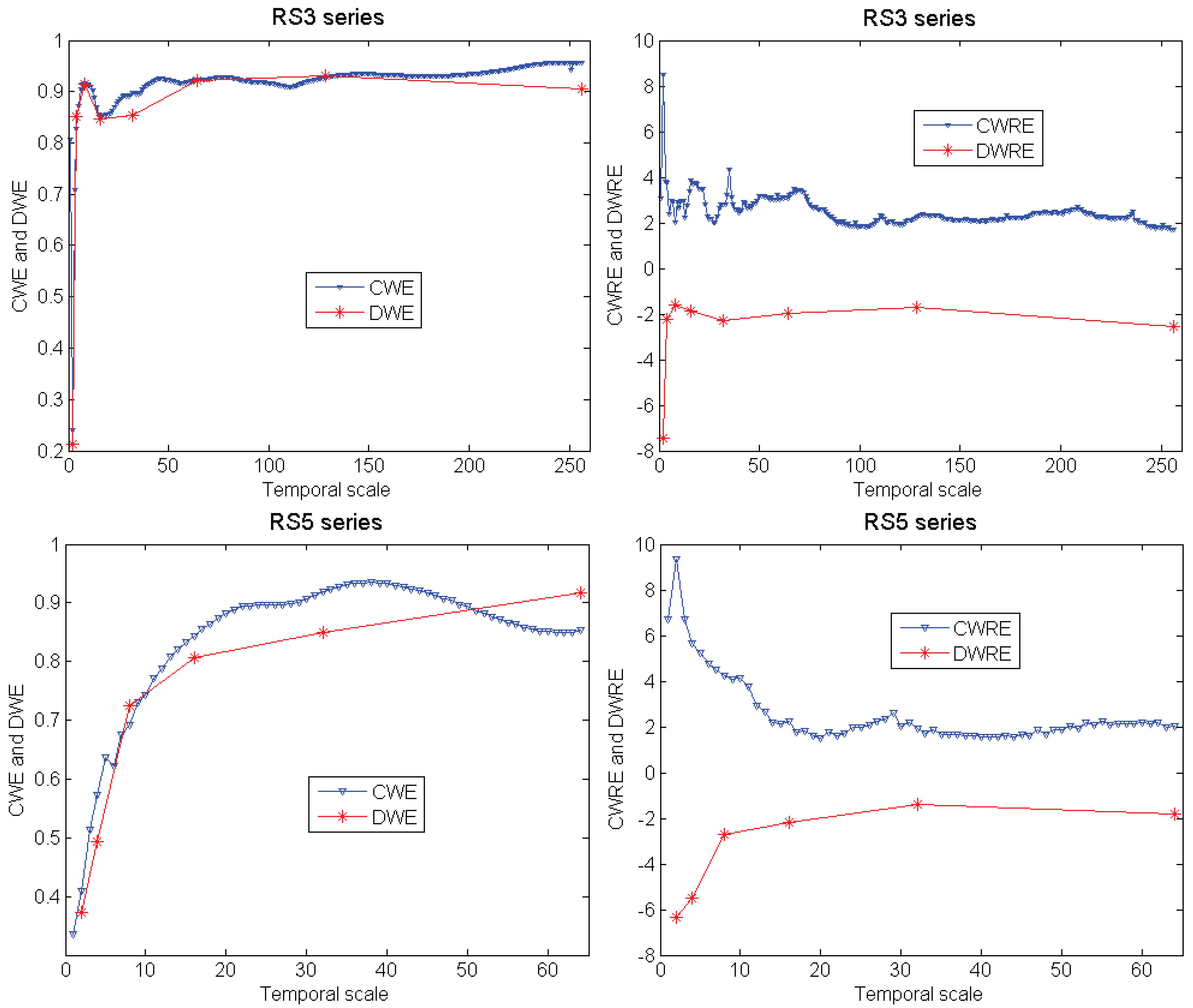
3.6. Comparison of Various Entropy Measures

After discussing the influence of four key issues on the calculation of wavelet-based entropy values, we use the RS3 and RS5 series as examples to further compare the performances of four wavelet-based entropy measures used in this paper. Concretely, we first analyze the de-noised RS3 and RS5 series by using CWT and dyadic DWT, respectively, based on which we quantify their complexities by using four entropy measures, namely CWE, CWRE, DWE and DWRE. The analytic results are depicted in Figure 6. It shows that the analytic results of CWE and DWE as a whole are close to each other under the whole temporal scales; the results of CWRE and DWRE are symmetrical to the zero-coordinate but also reflect the similar complexities of the two series. Therefore, it holds that the effectiveness of CWT is similar to that of DWT when used to analyze hydrologic series’ complexity. Besides, this is the reason for only using CWT in the above four sub-sections.
Furthermore, comparison results of Shannon entropy and relative entropy indicate that the latter is more effective. Because the values of wavelet-based relative entropy can denote the degree of similarity between the original series data and its sub-signal under certain TS (or DL), based on which we not only can quantify hydrologic series’ complexity more authentically, but also can clearly understand the characteristics and composition of hydrologic series data under multi-temporal scales. In the authors’ opinion, the deficiencies of CWE and DWE are mainly caused by the assumption of series’ random characters when using Shannon entropy. If a period exists under certain temporal scale, its complexity quantified by using CWE and DWE would be much bigger, which does not accord with the physical basis and thus is unreliable. We take the RS3 series with the dominant period of 12 months for example, the value of its CWE and DWE under the TS 12 are maximum with the value of bigger than 0.9; but its CWRE and DWRE under the TS 12 are minimum with the absolute value of smaller than −2; therefore the latter results are more reasonable. Besides, this conclusion can also be gained from the results of RS1 series in Figure 4, RS2 series in Figure 5 and RS4 in Figure 3.
By comprehensive analysis of these results, it can be concluded that CWT is as effective as DWT, but the relative entropy is better than conventional Shannon entropy in the analytic process of hydrologic series’ complexity. Therefore the performances of CWRE and DWRE are the best comparatively among the four entropy measures used in this paper.
Figure 6. Calculation results of wavelet-based entropy values (CWE, CWRE, DWE and DWRE) used to describe the complexities of de-noised RS3 and RS5 series.
Entropy 13 00195 g006

4. Conclusions

Quantification of the complexity of hydrologic series data under multi-temporal scales is the substantial issue in hydrologic series analysis. In this paper, we first studied the influence of four key issues on calculation of entropy values, and then compared the performances of four wavelet-based entropy measures used commonly. By comprehensively analyzing the results of various examples, several conclusions and suggestions gained in this study have been drawn as follows:
  • (1) Both the wavelet choice and noise have great influence on the quantification of hydrologic series’ complexity. It is suggested that the method of choosing wavelet in [26] be used in practice, because by using it both the appropriate wavelet and reliable de-noising results of hydrologic series data can be obtained.
  • (2) The estimation of probability density function is a key issue influencing the calculation of entropy values. Comparatively, the Type-II pdf is recommended, because it is based on the energy distribution of series data, and by using it the complexity of hydrologic series data under multi-temporal scales can be quantified more accurately and reasonably.
  • (3) The trend of hydrologic series also influences the calculation of entropy values. Therefore in the analytic process of hydrologic series’ complexity, the composition of series data, especially the trend, should be carefully taken into consideration.
  • (4) Analytic results of complexity of hydrologic series data vary with the entropy measures used. It is suggested that the wavelet-based relative entropy (CWRE and DWRE) be used in practice, because it can not only subtly quantify the complexity but also reveal the characteristics and composition of hydrologic series data.

Acknowledgements

The authors gratefully acknowledge the helpful review comments and suggestions on an earlier version of the manuscript by Peter Harremoes, and three anonymous reviewers. The RS3 and RS4 series data were kindly provided by M.G. Yang, and the RS5 series data were kindly provided by C.P. Ling. The authors also thank Fei-Fei Liu for her assistance in preparation of the manuscript. This study was supported by the National Natural Science Fund of China (No. 41071018, 41030746, 40725010, 40730635), Jiangsu Project Innovation for PhD Candidates (No. CX10B_018Z), and the Excellent Disciplines Leaders in Midlife-Youth Program of Nanjing University.

References

  1. Wagener, T.; Gupta, H.V. Model identification for hydrological forecasting under uncertainty. Stoch. Environ. Res. Risk Assess. 2005, 19, 378–387. [Google Scholar] [CrossRef]
  2. Ravines, R.R.; Schmidt, A.M.; Migon, H.S.; Renno, C.D. A joint model for rainfall-runoff: The case of Rio Grande Basin. J. Hydrol. 2008, 35, 189–200. [Google Scholar] [CrossRef]
  3. Sang, Y.F.; Wang, D.; Wu, J.C.; Zhu, Q.P.; Wang, L. The relation between periods’ identification and noises in hydrologic series data. J. Hydrol. 2009, 368, 165–177. [Google Scholar] [CrossRef]
  4. Hanson, R.T.; Newhouse, M.W.; Dettinger, M.D. A methodology to assess relations between climatic variability and variations in hydrologic time series in the southwestern United States. J. Hydrol. 2004, 287, 252–269. [Google Scholar] [CrossRef]
  5. Boyer, C.; Chaumont, D.; Chartier, I.; Roy, A.G. Impact of climate change on the hydrology of St. Lawrence tributaries. J. Hydrol. 2010, 384, 65–83. [Google Scholar] [CrossRef]
  6. Jones, R.N.; Chiew, F.H.S.; Boughton, W.C.; Zhang, L. Estimating the sensitivity of mean annual runoff to climate change using selected hydrological models. Adv. Water Resour. 2006, 29, 1419–1429. [Google Scholar] [CrossRef]
  7. Carsten, M.; Morton, C.; Ralf, K.; Gunter, M.; Harry, V.; Frank, W. Modeling the water balance of a mesoscale catchment basin using remotely sensed land cover data. J. Hydrol. 2008, 353, 322–334. [Google Scholar]
  8. Labat, D. Recent advances in wavelet analyses: Part 1. A review of concepts. J. Hydrol. 2005, 314, 275–288. [Google Scholar] [CrossRef]
  9. Li, Z.W.; Zhang, Y.K. Multi-scale entropy analysis of Mississippi river flow. Stoch. Environ. Res. Risk Assess. 2008, 22, 507–512. [Google Scholar] [CrossRef]
  10. Koutsoyiannis, D. Uncertainty, entropy, scaling and hydrological stochastics. 1. Marginal distributional properties of hydrological processes and state scaling. Hydrol. Sci. J. 2005, 50, 381–404. [Google Scholar]
  11. Brunsell, N.A. A multiscale information theory approach to assess spatial-temporal variability of daily precipitation. J. Hydrol. 2010, 385, 165–172. [Google Scholar] [CrossRef]
  12. Wang, D.; Singh, V.P.; Zhu, Y.S. Hybrid fuzzy and optimal modeling for water quality evaluation. Water Resour. Res. 2007, 43, W05415. [Google Scholar] [CrossRef]
  13. Jaynes, E.T. Information theory and statistical mechanics. Phys. Rev. 1957, 106, 620–630. [Google Scholar] [CrossRef]
  14. Elsner, J.; Tsonis, A. Complexity and predictability of hourly precipitation. J. Atmos. Sci. 1993, 50, 400–405. [Google Scholar] [CrossRef]
  15. Padmanabhan, G.; Rao, A.R. Maximum entropy spectral analysis of hydrologic data. Water Resour. Res. 1988, 24, 1519–1533. [Google Scholar] [CrossRef]
  16. Singh, V.P. Entropy-based Parameter Estimation in Hydrology; Kluwer Academic Publishers: Boston, MA, USA/London, UK, 1998. [Google Scholar]
  17. Zhang, Y.C. Complexity and 1/f noise: A phase space approach. J. Phys. I France 1991, 1, 971–977. [Google Scholar] [CrossRef]
  18. Costa, M.; Goldberger, A.L.; Peng, C.K. Multiscale entropy analysis of biological signals. Phys. Rev. E 2005, 71, 021906. [Google Scholar] [CrossRef]
  19. Percival, D.B.; Walden, A.T. Wavelet Methods for Time Series Analysis; Cambridge University Press: Cambridge, UK, 2000. [Google Scholar]
  20. Torrence, C.; Compo, G.P. A practical guide to wavelet analysis. Bull. Amer. Meteorol. Soc. 1998, 79, 61–78. [Google Scholar] [CrossRef]
  21. Zunino, L.; Perez, D.G.; Garavaglia, M.; Rosso, O.A. Wavelet entropy of stochastic processes. Phys. A 2007, 379, 503–512. [Google Scholar] [CrossRef]
  22. Emre Cek, M.; Ozgoren, M.; Acar Savaci, F. Continuous time wavelet entropy of auditory evoked potentials. Comput. Bio. Med. 2010, 40, 90–96. [Google Scholar] [CrossRef] [PubMed]
  23. Molini, A.; Barbera, P.L.; Lanza, L.G. Correlation patterns and information flows in rainfall fields. J. Hydrol. 2006, 322, 89–104. [Google Scholar] [CrossRef]
  24. Abramov, R.; Majda, A.; Kleeman, R. Information theory and predictability for low-frequency variability. J. Atmos. Sci. 2005, 62, 65–87. [Google Scholar] [CrossRef]
  25. Chui, C.K. Wavelet Analysis and Its Applications. In An Introduction to Wavelets; Academic Press: Boston, MA, USA, 1992; Volume 1. [Google Scholar]
  26. Sang, Y.F.; Wang, D.; Wu, J.C.; Zhu, Q.P.; Wang, L. Entropy-based wavelet de-noising method for time series analysis. Entropy 2009, 11, 1123–1147. [Google Scholar] [CrossRef]
  27. Sang, Y.F.; Wang, D.; Wu, J.C. Entropy-Based Method of Choosing the Decomposition Level in Wavelet Threshold De-noising. Entropy 2010, 6, 1499–1513. [Google Scholar] [CrossRef]
  28. Donoho, D.H. De-noising by soft-thresholding. IEEE Trans. Inform. Theory 1995, 41, 613–617. [Google Scholar] [CrossRef]
  29. Jansen, M. Minimum risk thresholds for data with heavy noise. IEEE Signal Process. Lett. 2006, 13, 296–299. [Google Scholar] [CrossRef]
  30. Chen, X.D.; Cao, S.L.; Wang, G.A.; Zhang, M.Q. Yellow River Hydrology; (in Chinese). The Publisher of Water Conservancy of the Yellow River: Zhengzhou, China, 1996. [Google Scholar]
  31. Schaefli, B.; Maraun, D.; Holschneider, M. What drives high flow events in the Swiss Alps? Recent developments in wavelet spectral analysis and their application to hydrology. Adv. Water Resour. 2007, 30, 2511–2525. [Google Scholar] [CrossRef]
  32. Alexander, M.E.; Baumgartner, R.; Summers, A.R.; Windischberger, C.; Klarhoefer, M.; Moser, E.; Somorjai, R.L. A wavelet-based method for improving signal-to-noise ratio and contrast in MR images. Magn. Reson. Imag. 2000, 18, 169–180. [Google Scholar] [CrossRef]
  33. Hrachowitz, M.; Soulsby, C.; Tetzlaff, D.; Dawson, J.J.C.; Dunn, S.M.; Malcolm, I.A. Using long-term data sets to understand transit times in contrasting headwater catchments. J. Hydrol. 2009, 367, 237–248. [Google Scholar] [CrossRef]
  34. Khan, T.; Ramuhalli, P.; Zhang, W.G.; Raveendra, S.T. De-noising and regularization in generalized NAH for turbomachinery acoustic noise source reconstruction. Noise Contr. Eng. J. 2010, 58, 93–103. [Google Scholar] [CrossRef]
  35. Sang, Y.F.; Wang, D.; Wu, J.C. Probabilistic forecast and uncertainty assessment of hydrologic design values using Bayesian theories. Hum. Ecol. Risk Assess. 2010, 16, 1184–1207. [Google Scholar] [CrossRef]

