The Michaelis-Menten-Stueckelberg Theorem

Abstract

We study chemical reactions with complex mechanisms under two assumptions: (i) intermediates are present in small amounts (this is the quasi-steady-state hypothesis or QSS) and (ii) they are in equilibrium relations with substrates (this is the quasiequilibrium hypothesis or QE). Under these assumptions, we prove the generalized mass action law together with the basic relations between kinetic factors, which are sufficient for the positivity of the entropy production but hold even without microreversibility, when the detailed balance is not applicable. Even though QE and QSS produce useful approximations by themselves, only the combination of these assumptions can render the possibility beyond the “rarefied gas” limit or the “molecular chaos” hypotheses. We do not use any a priori form of the kinetic law for the chemical reactions and describe their equilibria by thermodynamic relations. The transformations of the intermediate compounds can be described by the Markov kinetics because of their low density (low density of elementary events). This combination of assumptions was introduced by Michaelis and Menten in 1913. In 1952, Stueckelberg used the same assumptions for the gas kinetics and produced the remarkable semi-detailed balance relations between collision rates in the Boltzmann equation that are weaker than the detailed balance conditions but are still sufficient for the Boltzmann H-theorem to be valid. Our results are obtained within the Michaelis-Menten-Stueckelbeg conceptual framework.

1. Introduction

1.1. Main Asymptotic Ideas in Chemical Kinetics

There are several essentially different approaches to asymptotic and scale separation in kinetics, and each of them has its own area of applicability.

In chemical kinetics various fundamental ideas about asymptotical analysis were developed [1]: Quasieqiulibrium asymptotic (QE), quasi steady-state asymptotic (QSS), lumping, and the idea of limiting step.

Most of the works on nonequilibrium thermodynamics deal with the QE approximations and corrections to them, or with applications of these approximations (with or without corrections). There are two basic formulation of the QE approximation: The thermodynamic approach, based on entropy maximum, or the kinetic formulation, based on selection of fast reversible reactions. The very first use of the entropy maximization dates back to the classical work of Gibbs [2], but it was first claimed for a principle of informational statistical thermodynamics by Jaynes [3]. A very general discussion of the maximum entropy principle with applications to dissipative kinetics is given in the review [4]. Corrections of QE approximation with applications to physical and chemical kinetics were developed [5,6].

QSS was proposed by Bodenstein in 1913 [7], and the important Michaelis and Menten work [8] was published simultaneously. It appears that no kinetic theory of catalysis is possible without QSS. This method was elaborated into an important tool for the analysis of chemical reaction mechanism and kinetics [9,10,11]. The classical QSS is based on the relative smallness of concentrations of some of the “active” reagents (radicals, substrate-enzyme complexes or active components on the catalyst surface) [12,13,14].

Lumping analysis aims to combine reagents into “quasicomponents” for dimension reduction [15,17,18,19]. Wei and Prater [16] demonstrated that for (pseudo)monomolecular systems there exist linear combinations of concentrations which evolve in time independently. These linear combinations (quasicomponents) correspond to the left eigenvectors of the kinetic matrix: If $lK=\lambda l$ then $\mathrm{d}(l,c)/\mathrm{d}t=(l,c)\lambda$, where the standard inner product $(l,c)$ is the concentration of a quasicomponent. They also demonstrated how to find these quasicomponents in a properly organized experiment.

This observation gave rise to a question: How to lump components into proper quasicomponents to guarantee the autonomous dynamics of the quasicomponents with appropriate accuracy? Wei and Kuo studied conditions for exact [15] and approximate [17] lumping in monomolecular and pseudomonomolecular systems. They demonstrated that under certain conditions a large monomolecular system could be well-modelled by a lower-order system.

More recently, sensitivity analysis and Lie group approach were applied to lumping analysis [18,19], and more general nonlinear forms of lumped concentrations were used (for example, concentration of quasicomponents could be a rational function of c).

Lumping analysis was placed in the linear systems theory and the relationships between lumpability and the concepts of observability, controllability and minimal realization were demonstrated [20]. The lumping procedures were considered also as efficient techniques leading to nonstiff systems and demonstrated the efficiency of the developed algorithm on kinetic models of atmospheric chemistry [21]. An optimal lumping problem can be formulated in the framework of a mixed integer nonlinear programming (MINLP) and can be efficiently solved with a stochastic optimization method [22].

The concept of limiting step gives the limit simplification: The whole network behaves as a single step. This is the most popular approach for model simplification in chemical kinetics and in many areas beyond kinetics. In the form of a bottleneck approach this approximation is very popular from traffic management to computer programming and communication networks. Recently, the concept of the limiting step has been extended to the asymptotology of multiscale reaction networks [23,24].

In this paper, we focus on the combination of the QE approximation with the QSS approach.

1.2. The Structure of the Paper

Almost thirty years ago one of us published a book [25] with Chapter 3 entitled “Quasiequilibrium and Entropy Maximum”. A research program was formulated there, and now we are in the position to analyze the achievements of these three decades and formulate the main results, both theoretical and applied, and the unsolved problems. In this paper, we start this work and combine a presentation of theory and application of the QE approximation in physical and chemical kinetics with exposition of some new results.

We start from the formal description of the general idea of QE and its possible extensions. In Section 2, we briefly introduce main notations and some general formulas for exclusion of fast variables by the QE approximation.

In Section 3, we present the history of the QE and the classical confusion between the QE and the quasi steady state (QSS) approximation. Another surprising confusion is that the famous Michaelis-Menten kinetics was not proposed by Michaelis and Menten in 1913 [8] but by Briggs and Haldane [12] in 1925. It is more important that Michaelis and Menten proposed another approximation that is very useful in general theoretical constructions. We described this approximation for general kinetic systems. Roughly speaking, this approximation states that any reaction goes through transformation of fast intermediate complexes (compounds), which (i) are in equilibrium with the input reagents and (ii) exist in a very small amount.

One of the most important benefits from this approach is the exclusion of nonlinear kinetic laws and reaction rate constants for nonlinear reactions. The nonlinear reactions transform into the reactions of the compounds production. They are in a fast equilibrium and the equilibrium is ruled by thermodynamics. For example, when Michaelis and Menten discuss the production of the enzyme-substrate complex ES from enzyme E and substrate S, they do not discuss reaction rates. These rates may be unknown. They just assume that the reaction $E+S\rightleftharpoons ES$ is in equilibrium. Briggs and Haldane involved this reaction into the kinetic model. Their approach is more general than the Michaelis-Menten approximation but for the Briggs and Haldane model we need more information, not only the equilibrium of the reaction $E+S\rightleftharpoons ES$ but also its rates and constants.

When compounds undergo transformations in a linear first order kinetics, there is no need to include interactions between them because they are present in very small amounts in the same volume, and their concentrations are also small. (By the way, this argument is not applicable to the heterogeneous catalytic reactions. Although the intermediates are in both small amounts and in a small volume, i.e., in the surface layer, the concentration of the intermediates is not small, and their interaction does not vanish when their amount decreases [33]. Therefore, kinetics of intermediates in heterogeneous catalysis may be nonlinear and demonstrate bifurcations, oscillations and other complex behavior.)

In 1952, Stueckelberg [26] used similar approach in his seminal paper “H-theorem and unitarity of the S-matrix”. He studied elastic collisions of particles as the quasi-chemical reactions

$$\mathrm{v}+\mathrm{w}\to {\mathrm{v}}^{\prime }+{\mathrm{w}}^{\prime }$$

($\mathrm{v},\mathrm{w},{\mathrm{v}}^{\prime },{\mathrm{w}}^{\prime }$ are velocities of particles) and demonstrated that for the Boltzmann equation the linear Markov kinetics of the intermediate compounds results in the special relations for the kinetic coefficients. These relations are sufficient for the H-theorem, which was originally proved by Boltzmann under the stronger assumption of reversibility of collisions [27].

First, the idea of such relations was proposed by Boltzmann as an answer to the Lorentz objections against Boltzmann’s proof of the H-theorem. Lorentz stated the nonexistence of inverse collisions for polyatomic molecules. Boltzmann did not object to this argument but proposed the “cyclic balance” condition, which means balancing in cycles of transitions between states $S_1\to S_2\to \dots \to S_n\to S_1$. Almost 100 years later, Cercignani and Lampis [28] demonstrated that the Lorenz arguments are wrong and the new Boltzmann relations are not needed for the polyatomic molecules under the microreversibility conditions. The detailed balance conditions should hold.

Nevertheless, Boltzmann’s idea is very seminal. It was studied further by Heitler [29] and Coester [30] and the results are sometimes cited as the “Heitler-Coestler theorem of semi-detailed balance”. In 1952, Stueckelberg [26] proved these conditions for the Boltzmann equation. For the micro-description he used the S-matrix representation, which is in this case equivalent for the Markov microkinetics (see also [31]).

Later, these relations for the chemical mass action kinetics were rediscovered and called the complex balance conditions [51,63]. We generalize the Michaelis-Menten-Stueckelberg approach and study in Section 5 the general kinetics with fast intermediates present in small amount. In SubSection 5.7 the big Michaelis-Menten-Stueckelberg theorem is formulated as the overall result of the previous analysis.

Before this general theory, we introduce the formalism of the QE approximation with all the necessary notations and examples for chemical kinetics in Section 4.

The result of the general kinetics of systems with intermediate compounds can be used wider than this specific model of an elementary reaction: The intermediate complexes with fast equilibria and the Markov kinetics can be considered as the “construction staging” for general kinetics. In Section 6, we delete the construction staging and start from the general forms of the obtained kinetic equations as from the basic laws. We study the relations between the general kinetic law and the thermodynamic condition of the positivity of the entropy production.

Sometimes the kinetics equations may not respect thermodynamics from the beginning. To repair this discrepancy, deformation of the entropy may help. In Section 7, we show when is it possible to deform the entropy by adding a linear function to provide agreement between given kinetic equations and the deformed thermodynamics. As a particular case, we got the “deficiency zero theorem”.

The classical formulation of the principle of detailed balance deals not with the thermodynamic and global forms we use but just with equilibria: In equilibrium each process must be equilibrated with its reverse process. In Section 7, we demonstrate also that for the general kinetic law the existence of a point of detailed balance is equivalent to the existence of such a linear deformation of the entropy that the global detailed balance conditions (Equation (87) below) hold. Analogously, the existence of a point of complex balance is equivalent to the global condition of complex balance after some linear deformation of the entropy.

1.3. Main Results: One Asymptotic and Two Theorems

Let us follow the ideas of Michaelis-Menten and Stueckelberg and introduce the asymptotic theory of reaction rates. Let the list of the components $A_i$ be given. The mechanism of reaction is the list of the elementary reactions represented by their stoichiometric equations:

$$\sum _i{\alpha }_{\rho i}{A}_i\to \sum _i{\beta }_{\rho i}{A}_i$$

(1)

The linear combinations ${\sum }_i{\alpha }_{\rho i}{A}_i$ and ${\sum }_i{\beta }_{\rho i}{A}_i$ are the complexes. For each complex ${\sum }_i{y}_{ji}{A}_i$ from the reaction mechanism we introduce an intermediate auxiliary state, a compound $B_j$. Each elementary reaction is represented in the form of the “$2n$-tail scheme” (Figure 1) with two intermediate compounds:

$$\sum _i{\alpha }_{\rho i}{A}_i\rightleftharpoons B_{\rho }^{-}\to B_{\rho }^{+}\rightleftharpoons \sum _i{\beta }_{\rho i}{A}_i$$

(2)

There are two main assumptions in the Michaelis-Menten-Stueckelberg asymptotic:

• The compounds are in fast equilibrium with the corresponding input reagents (QE);
• They exist in very small concentrations compared to other components (QSS).

The smallness of the concentration of the compounds implies that they (i) have the perfect thermodynamic functions (entropy, internal energy and free energy) and (ii) the rates of the reactions $B_i\to B_j$ are linear functions of their concentrations.

One of the most important benefits from this approach is the exclusion of the nonlinear reaction kinetics: They are in fast equilibrium and equilibrium is ruled by thermodynamics.

Under the given smallness assumptions, the reaction rates $r_{\rho }$ for the elementary reactions have a special form of the generalized mass action law (see Equation (74) below):

$$r_{\rho }={\phi }_{\rho }exp({\alpha }_{\rho },\check{\mu })$$

where ${\phi }_{\rho }>0$ is the kinetic factor and $exp({\alpha }_{\rho },\check{\mu })$ is the Boltzmann factor. Here and further in the text $({\alpha }_{\rho },\check{\mu })={\sum }_i{\alpha }_{\rho i}{\check{\mu }}_i$ is the standard inner product, $exp(,)$ is the exponential of the value of the inner product and ${\check{\mu }}_i$ are chemical potentials μ divided on $RT$.

For the prefect chemical systems, ${\check{\mu }}_i=ln(c_i/c_i^{*})$, where $c_i$ is the concentration of $A_i$ and $c_i^{*}>0$ are the positive equilibrium concentrations. For different values of the conservation laws there are different positive equilibria. The positive equilibrium $c_i^{*}$ is one of them and it is not important which one is it. At this point, ${\check{\mu }}_i=0$, hence, the kinetic factor for the perfect systems is just the equilibrium value of the rate of the elementary reaction at the equilibrium point $c^{*}$: ${\phi }_{\rho }=r_{\rho }\left(c^{*}\right)$.

The linear kinetics of the compound reactions $B_i\to B_j$ implies the remarkable identity for the reaction rates, the complex balance condition (Equation (89) below)

$$\sum _{\rho }{\phi }_{\rho }exp(\check{\mu },{\alpha }_{\rho })=\sum _{\rho }{\phi }_{\rho }exp(\check{\mu },{\beta }_{\rho })$$

for all admissible values of $\check{\mu }$ and given ϕ which may vary independently. For other and more convenient forms of this condition see Equation (91) in Section 6. The complex balance condition is sufficient for the positivity of the entropy production (for decrease of the free energy under isothermal isochoric conditions). The general formula for the reaction rate together with the complex balance conditions and the positivity of the entropy production form the Michaelis-Menten-Stueckelberg theorem (Section 5.7).

The detailed balance conditions (Equation (87) below),

$${\phi }_{\rho }^{+}={\phi }_{\rho }^{-}$$

for all ρ, are more restrictive than the complex balance conditions. For the perfect systems, the detailed balance condition takes the standard form: $r_{\rho }^{+}\left(c^{*}\right)=r_{\rho }^{-}\left(c^{*}\right)$.

We study also some other, less restrictive sufficient conditions for accordance between thermodynamics and kinetics. For example, we demonstrate that the G-inequality (Equation (92) below)

$$\sum _{\rho }{\phi }_{\rho }exp(\check{\mu },{\alpha }_{\rho })\ge \sum _{\rho }{\phi }_{\rho }exp(\check{\mu },{\beta }_{\rho })$$

is sufficient for the entropy growth and, at the same time, weaker than the condition of complex balance.

If the reaction rates have the form of the generalized mass action law but do not satisfy the sufficient condition of the positivity of the entropy production, the situation may be improved by the deformation of the entropy via addition of a linear function. Such a deformation is always possible for the zero deficiency systems. Let q be the number of different complexes in the reaction mechanism, d be the number of the connected components in the digraph of the transitions between compounds (vertices are compounds and edges are reactions). To exclude some degenerated cases a hypothesis of weak reversibility is accepted: For any two vertices $B_i$ and $B_j$, the existence of an oriented path from $B_i$ to $B_j$ implies the existence of an oriented path from $B_j$ to $B_i$.

Deficiency of the system is [63]

$$q-d-\mathrm{rank}\Gamma \ge 0$$

where $\Gamma =\left({\gamma }_{ij}\right)=({\beta }_{ij}-{\alpha }_{ij})$ is the stoichiometric matrix. If the system has zero deficiency then the entropy production becomes positive after the deformation of the entropy via addition of a linear function. The deficiency zero theorem in this form is proved in Section 7.3.

Interrelations between the Michaelis-Menten-Stueckelberg asymptotic and the transition state theory (which is also referred to as the “activated-complex theory”, “absolute-rate theory”, and “theory of absolute reaction rates”) are very intriguing. This theory was developed in 1935 by Eyring [35] and by Evans and Polanyi [36].

Basic ideas behind the transition state theory are [37]:

• The activated complexes are in a quasi-equilibrium with the reactant molecules;
• Rates of the reactions are studied by studying the activated complexes at the saddle point of a potential energy surface.

The similarity is obvious but in the Michaelis-Menten-Stueckelberg asymptotic an elementary reaction is represented by a couple of compounds with the Markov kinetics of transitions between them versus one transition state, which moves along the “reaction coordinate”, in the transition state theory. This is not exactly the same approach (for example, the theory of absolute reaction rates uses the detailed balance conditions and does not produce anything similar to the complex balance).

Important technical tools for the analysis of the Michaelis-Menten-Stueckelberg asymptotic are the theorem about preservation of the entropy production in the QE approximation (Section 2 and Appendix 1) and the Morimoto H-theorem for the Markov chains (Appendix 2).

2. QE and Preservation of Entropy Production

In this section we introduce informally the QE approximation and the important theorem about the preservation of entropy production in this approximation. In Appendix 1, this approximation and the theorem are presented with more formal details.

Let us consider a system in a domain U of a real vector space E given by differential equations

$$\frac{\mathrm{d}x}{\mathrm{d}t}=F\left(x\right)$$

(3)

The QE approximation for (3) uses two basic entities: Entropy and slow variables.

Entropy S is an increasing concave Lyapunov function for (3) with non-degenerated Hessian ${\partial }^{2}S/\partial x_i\partial x_j$:

$$\frac{\mathrm{d}S}{\mathrm{d}t}\ge 0$$

(4)

In this approach, the increase of entropy in time is exploited (the Second Law in the form (4)).

The slow variables M are defined as some differentiable functions of variables x: $M=m\left(x\right)$. Here we assume that these functions are linear. More general nonlinear theory was developed in [38,39] with applications to the Boltzmann equation and polymer physics. Selection of the slow variables implies a hypothesis about separation of fast and slow motion. The slow variables (almost) do not change during the fast motion. After some initial time, the fast variables with high accuracy are functions of the slow variables: We can write $x\approx x_M^{*}$.

The QE approximation defines the functions $x_M^{*}$ as solutions to the following MaxEnt optimization problem:

$$S\left(x\right)\to max\mathrm{subject} \mathrm{to}m\left(x\right)=M$$

(5)

The reasoning behind this approximation is simple: During the fast initial layer motion, entropy increases and M almost does not change. Therefore, it is natural to assume that $x_M^{*}$ is close to the solution to the MaxEnt optimization problem (5). Further $x_M^{*}$ denotes a solution to the MaxEnt problem.

A solution to (5), $x_M^{*}$, is the QE state, the set of the QE states $x_M^{*}$, parameterized by the values of the slow variables M is the QE manifold, the corresponding value of entropy

$$S^{*}\left(M\right)=S\left(x_M^{*}\right)$$

(6)

is the QE entropy and the equation for the slow variables

$$\frac{\mathrm{d}M}{\mathrm{d}t}=m\left(F\left(x_M^{*}\right)\right)$$

(7)

represents the QE dynamics.

The crucial property of the QE dynamics is the preservation of entropy production.

Theorem about preservation of entropy production. 

Let us calculate $\mathrm{d}{S}^{*}\left(M\right)/\mathrm{d}t$ at point M according to the QE dynamics (7) and find $\mathrm{d}S\left(x\right)/\mathrm{d}t$ at point $x=x_M^{*}$ due to the initial system (3). The results always coincide:

$$\frac{\mathrm{d}{S}^{*}\left(M\right)}{\mathrm{d}t}=\frac{\mathrm{d}S\left(x\right)}{\mathrm{d}t}$$

(8)

The left hand side in (8) is computed due to the QE approximation (7) and the right hand side corresponds to the initial system (3). The sketch of the proof is given in Appendix 1.

The preservation of the entropy production leads to the preservation of the type of dynamics: If for the initial system (3) entropy production is non-negative, $\mathrm{d}S/\mathrm{d}t\ge 0$, then for the QE approximation (7) the production of the QE entropy is also non-negative, $\mathrm{d}{S}^{*}/\mathrm{d}t\ge 0$.

In addition, if for the initial system ${(\mathrm{d}S/\mathrm{d}t)|}_x=0$ if and only if $F\left(x\right)=0$ then the same property holds in the QE approximation.

3. The Classics and the Classical Confusion

3.1. The Asymptotic of Fast Reactions

It is difficult to find who introduced the QE approximation. It was impossible before the works of Boltzmann and Gibbs, and it became very well known after the works of Jaynes [3].

Chemical kinetics has been a source for model reduction ideas for decades. The ideas of QE appear there very naturally: Fast reactions go to their equilibrium and, after that, remain almost equilibrium all the time. The general formalization of this idea looks as follows. The kinetic equation has the form

$$\frac{\mathrm{d}N}{\mathrm{d}t}=K_{sl}\left(N\right)+\frac{1}{ϵ}{K}_{fs}\left(N\right)$$

(9)

Here N is the vector of composition with components $N_i>0$, $K_{sl}$ corresponds to the slow reactions, $K_{fs}$ corresponds to fast reaction and $ϵ>0$ is a small number. The system of fast reactions has the linear conservation laws $b_l\left(N\right)={\sum }_j{b}_{lj}{N}_j$: $b_l\left(K_{fs}\left(N\right)\right)\equiv 0$.

The fast subsystem

$$\frac{\mathrm{d}N}{\mathrm{d}t}=K_{fs}\left(N\right)$$

tends to a stable positive equilibrium $N^{*}$ for any positive initial state $N\left(0\right)$ and this equilibrium is a function of the values of the linear conservation laws $b_l\left(N\left(0\right)\right)$. In the plane $b_l\left(N\right)=b_l\left(N\left(0\right)\right)$ the equilibrium is asymptotically stable and exponentially attractive.

Vector $b\left(N\right)=\left(b_l\left(N\right)\right)$ is the vector of slow variables and the QE approximation is

$$\frac{\mathrm{d}b}{\mathrm{d}t}=b(K_{sl}\left(N^{*}\left(b\right)\right)$$

(10)

In chemical kinetics, equilibria can be described by conditional entropy maximum (or conditional extremum of other thermodynamic potentials). Therefore, for these cases we can apply the formalism of the quasiequilibrium approximation. The thermodynamic Lyapunov functions serve as tools for stability analysis and for model reduction [40].

The QE approximation, the asymptotic of fast reactions, is well known in chemical kinetics. Another very important approximation was invented in chemical kinetics as well. It is the Quasi Steady State (QSS) approximation. QSS was proposed in [7] and was elaborated into an important tool for analysis of chemical reaction mechanisms and kinetics [9,10,11]. The classical QSS is based on the relative smallness of concentrations of some of “active” reagents (radicals, substrate-enzyme complexes or active components on the catalyst surface) [13,14]. In the enzyme kinetics, its invention was traditionally connected to the so-called Michaelis-Menten kinetics.

3.2. QSS and the Briggs-Haldane Asymptotic

Perhaps the first very clear explanation of the QSS was given by Briggs and Haldane in 1925 [12]. Briggs and Haldane consider the simplest enzyme reaction $S+E\leftrightharpoons SE\to P+E$ and mention that the total concentration of enzyme ($\left[E\right]+\left[SE\right]$) is “negligibly small” compared with the concentration of substrate $\left[S\right]$. After that they conclude that $\frac{\mathrm{d}}{\mathrm{d}t}\left[SE\right]$ is “negligible” compared with $\frac{\mathrm{d}}{\mathrm{d}t}\left[S\right]$ and $\frac{\mathrm{d}}{\mathrm{d}t}\left[P\right]$ and produce the now famous ‘Michaelis-Menten’ formula, which was unknown to Michaelis and Menten: $k_1\left[E\right]\left[S\right]=(k_{-1}+k_2)\left[ES\right]$ or

$$\left[ES\right]=\frac{\left[E\right]\left[S\right]}{K_M+\left[S\right]}\mathrm{and}\frac{\mathrm{d}}{\mathrm{d}t}\left[P\right]=k_2\left[ES\right]=\frac{k_2\left[E\right]\left[S\right]}{K_M+\left[S\right]}$$

(11)

where the “Michaelis-Menten constant” is

$$K_M=\frac{k_{-1}+k_2}{k_1}$$

There is plenty of misleading comments in later publications about QSS. Two most important confusions are:

• Enzymes (or catalysts, or radicals) participate in fast reactions and, hence, relax faster than substrates or stable components. This is obviously wrong for many QSS systems: For example, in the Michaelis-Menten system all reactions include enzyme together with substrate or product. There are no separate fast reactions for enzyme without substrate or product.
• Concentrations of intermediates are constant because in QSS we equate their time derivatives to zero. In general case, this is also wrong: We equate the kinetic expressions for some time derivatives to zero, indeed, but this just exploits the fact that the time derivatives of intermediates concentrations are small together with their values, but not obligatory zero. If we accept QSS then these derivatives are not zero as well: To prove this we can just differentiate the Michaelis-Menten formula (11) and find that [ES] in QSS is almost constant when $\left[S\right]\gg K_M$, this is an additional condition, different from the Briggs-Haldane condition $\left[E\right]+\left[AE\right]\ll \left[S\right]$ (for more details see [1,14,33] and a simple detailed case study [41]).

After a simple transformation of variables the QSS smallness of concentration transforms into a separation of time scales in a standard singular perturbation form (see, for example [33,34]). Let us demonstrate this on the traditional Michaelis-Menten system:

$$\begin{array}{c}\frac{\mathrm{d}\left[S\right]}{\mathrm{d}t}=-k_1\left[S\right]\left[E\right]+k_{-1}\left[SE\right]\hfill \\ \frac{\mathrm{d}\left[SE\right]}{\mathrm{d}t}=k_1\left[S\right]\left[E\right]-(k_{-1}+k_2)\left[SE\right]\hfill \\ \left[E\right]+\left[SE\right]=e=const,\left[S\right]+\left[P\right]=s=const\hfill \end{array}$$

(12)

This is a homogeneous system with the isochoric (fixed volume) conditions for which we write the equations. The Briggs-Haldane condition is $e\ll s$. Let us use dimensionless variables $x=\left[S\right]/s$, $\xi =\left[SE\right]/e$:

$$\begin{array}{c}\frac{s}{e}\frac{\mathrm{d}x}{\mathrm{d}t}=-s{k}_{1}x(1-\xi )+k_{-1}\xi \hfill \\ \frac{\mathrm{d}\xi }{\mathrm{d}t}=s{k}_{1}x(1-\xi )-(k_{-1}+k_2)\xi \hfill \end{array}$$

(13)

To obtain the standard singularly perturbed system with the small parameter at the derivative, we need to change the time scale. This means that when $e\to 0$ the reaction goes proportionally slower and to study this limit properly we have to adjust the time scale: $\mathrm{d}\tau =\frac{e}{s}\mathrm{d}t$:

$$\begin{array}{c}\frac{\mathrm{d}x}{\mathrm{d}\tau }=-s{k}_{1}x(1-\xi )+k_{-1}\xi \hfill \\ \frac{e}{s}\frac{\mathrm{d}\xi }{\mathrm{d}\tau }=s{k}_{1}x(1-\xi )-(k_{-1}+k_2)\xi \hfill \end{array}$$

(14)

For small $e/s$, the second equation is a fast subsystem. According to this fast equation, for a given constant x, the variable ξ relaxes to

$${\xi }_{\mathrm{QSS}}=\frac{sx}{K_M+sx}$$

exponentially, as $exp(-(s{k}_{1}x+k_{-1}+k_2)t)$. Therefore, the classical singular perturbation theory based on the Tikhonov theorem [42,43] can be applied to the system in the form (14) and the QSS approximation is applicable even on an infinite time interval [44]. This transformation of variables and introduction of slow time is a standard procedure for rigorous proof of QSS validity in catalysis [33], enzyme kinetics [45] and other areas of kinetics and chemical engineering [13].

It is worth to mention that the smallness of parameter $e/s$ can be easily controlled in experiments, whereas the time derivatives, transformation rates and many other quantities just appear as a result of kinetics and cannot be controlled directly.

3.3. The Michaelis and Menten Asymptotic

QSS is not QE but the classical work of Michaelis and Menten [8] was done on the intersection of QSS and QE. After the brilliantly clear work of Briggs and Haldane, the name “Michaelis-Menten” was attached to the Briggs and Haldane equation and the original work of Michaelis and Menten was considered as an important particular case of this approach, an approximation with additional and not necessary assumptions of QE. From our point of view, the Michaelis-Menten work includes more and may give rise to an important general class of kinetic models.

Michaelis and Menten studied the “fermentative splitting of cane sugar”. They introduced three “compounds”: The sucrose-ferment combination, the fructose-ferment combination and the glucose-ferment combination. The fundamental assumption of their work was “that the rate of breakdown at any moment is proportional to the concentration of the sucrose-invertase compound”.

They started from the assumption that at any moment according to the mass action law

$$\left[S_i\right]\left[E\right]=K_i\left[S_{i}E\right]$$

(15)

where $\left[S_i\right]$ is the concentration of the ith sugar (here, $i=0$ for sucrose, 1 for fructose and 2 for glucose), $\left[E\right]$ is the concentration of the free invertase and $K_i$ is the ith equilibrium constant.

For simplification, they use the assumption that the concentration of any sugar in question in free state is practically equal to that of the total sugar in question.

Finally, they obtain

$$\left[S_{0}E\right]=\frac{e\left[S_0\right]}{K_0(1+q\left[P\right])+\left[S_0\right]}$$

(16)

where $e=\left[E\right]+{\sum }_i\left[S_{i}E\right]$, $\left[P\right]=\left[S_1\right]=\left[S_2\right]$ and $q=\frac{1}{K_1}+\frac{1}{K_2}$.

Of course, this formula may be considered as a particular case of the Briggs-Haldane formula (11) if we take $k_{-1}\gg k_2$ in (11) (i.e., the equilibration $S+E\leftrightharpoons SE$ is much faster than the reaction $SE\to P+E$) and assume that $q=0$ in (16) (i.e., fructose-ferment combination and glucose-ferment combination are practically absent).

This is the truth but may be not the complete truth. The Michaelis-Menten approach with many compounds which are present in small amounts and satisfy the QE assumption (15) is a seed of the general kinetic theory for perfect and non-perfect mixtures.

4. Chemical Kinetics and QE Approximation

4.1. Stoichiometric Algebra and Kinetic Equations

In this section, we introduce the basic notations of the chemical kinetics formalism. For more details see, for example, [33].

The list of components is a finite set of symbols $A_1,\dots ,A_n$.

A reaction mechanism is a finite set of the stoichiometric equations of elementary reactions:

$$\sum _i{\alpha }_{\rho i}{A}_i\to \sum _i{\beta }_{\rho i}{A}_i$$

(17)

where $\rho =1,\dots ,m$ is the reaction number and the stoichiometric coefficients ${\alpha }_{\rho i},{\beta }_{\rho i}$ are nonnegative integers.

A stoichiometric vector ${\gamma }_{\rho }$ of the reaction (17) is a n-dimensional vector with coordinates

$${\gamma }_{\rho i}={\beta }_{\rho i}-{\alpha }_{\rho i}$$

(18)

that is, “gain minus loss” in the ρth elementary reaction.

A nonnegative extensive variable $N_i$, the amount of $A_i$, corresponds to each component. We call the vector N with coordinates $N_i$ “the composition vector”. The concentration of $A_i$ is an intensive variable $c_i=N_i/V$, where $V>0$ is the volume. The vector $c=N/V$ with coordinates $c_i$ is the vector of concentrations.

A non-negative intensive quantity, $r_{\rho }$, the reaction rate, corresponds to each reaction (17). The kinetic equations in the absence of external fluxes are

$$\frac{\mathrm{d}N}{\mathrm{d}t}=V\sum _{\rho }{r}_{\rho }{\gamma }_{\rho }$$

(19)

If the volume is not constant then equations for concentrations include $\dot{V}$ and have different form (this is typical for the combustion reactions, for example).

For perfect systems and not so fast reactions, the reaction rates are functions of concentrations and temperature given by the mass action law for the dependance on concentrations and by the generalized Arrhenius equation for the dependance on temperature T.

The mass action law states:

$$r_{\rho }(c,T)=k_{\rho }\left(T\right)\prod _i{c}_i^{{\alpha }_{\rho i}}$$

(20)

where $k_{\rho }\left(T\right)$ is the reaction rate constant.

The generalized Arrhenius equation is:

$$k_{\rho }\left(T\right)=A_{\rho }{\left(\frac{T}{T_0}\right)}^{\frac{S_{\mathrm{a}\rho }}{R}}exp\left(-\frac{E_{\mathrm{a}\rho }}{RT}\right)$$

(21)

where $R=8.314472\frac{\mathrm{J}}{\mathrm{K}\mathrm{mol}}$ is the universal, or ideal gas constant, $E_{\mathrm{a}\rho }$ is the activation energy, $S_{\mathrm{a}\rho }$ is the activation entropy (i.e., $E_{\mathrm{a}\rho }-T{S}_{\mathrm{a}\rho }$ is the activation free energy), $A_{\rho }$ is the constant pre-exponential factor. Some authors neglect the $S_{\mathrm{a}\rho }$ term because it may be less important than the activation energy, but it is necessary to stress that without this term it may be impossible to reconcile the kinetic equations with the classical thermodynamics.

In general, the constants for different reactions are not independent. They are connected by various conditions that follow from thermodynamics (the second law, the entropy growth for isolated systems) or microreversibility assumption (the detailed balance and the Onsager reciprocal relations). In Section 6.2 we discuss these conditions in more general settings.

For nonideal systems, more general kinetic law is needed. In Section 5 we produce such a general law following the ideas of the original Michaelis and Menten paper (this is not the same as the famous “Michaelis-Menten kinetics”). For this work we need a general formalism of QE approximation for chemical kinetics.

4.2. Formalism of QE Approximation for Chemical Kinetics

4.2.1. QE Manifold

In this section, we describe the general formalism of the QE for chemical kinetics following [34].

The general construction of the quasi-equilibrium manifold gives the following procedure. First, let us consider the chemical reactions in a constant volume under the isothermal conditions. The free energy $F(N,T)=Vf(c,T)$ should decrease due to reactions. In the space of concentrations, one defines a subspace of fast motions L. It should be spanned by the stoichiometric vectors of fast reactions.

Slow coordinates are linear functions that annulate L. These functions form a subspace in the space of linear functions on the concentration space. Dimension of this space is $s=n-dimL$. It is necessary to choose any basis in this subspace. We can use for this purpose a basis $b_j$ in $L^{\perp }$, an orthogonal complement to L and define the basic functionals as $b_j\left(N\right)=(b_j,N)$.

The description of the QE manifold is very simple in the Legendre transform. The chemical potentials are partial derivatives

$${\mu }_i=\frac{\partial F(N,T)}{\partial N_i}=\frac{\partial f(c,T)}{\partial c_i}$$

(22)

Let us use ${\mu }_i$ as new coordinates. In these new coordinates (the “conjugated coordinates”), the QE manifold is just an orthogonal complement to L. This subspace, $L^{\perp }$, is defined by equations

$$\sum _i{\mu }_i{\gamma }_i=0\mathrm{for}\mathrm{any}\gamma \in L$$

(23)

It is sufficient to take in (23) not all $\gamma \in L$ but only elements from a basis in L. In this case, we get the system of $n-dimL$ linear equations of the form (23) and their solution does not cause any difficulty. For the actual computations, one requires the inversion from μ to c.

It is worth to mention that the problems of the selection of the slow variables and of the description of the QE manifold in the conjugated variables can be considered as the same problem of description of the orthogonal complement, $L^{\perp }$.

To finalize the construction of the QE approximation, we should find for any given values of slow variables (and of conservation laws) $b_i$ the corresponding point on the QE manifold. This means that we have to solve the system of equations for c:

$$b\left(N\right)=b;(\mu (c,T),{\gamma }_{\rho })=0$$

(24)

where b is the vector of slow variables, μ is the vector of chemical potentials and vectors ${\gamma }_{\rho }$ form a basis in L. After that, we have the QE dependence $c_{QE}\left(b\right)$ and for any admissible value of b we can find all the reaction rates and calculate $\dot{b}$.

Unfortunately, the system (24) can be solved analytically only in some special cases. In general case, we have to solve it numerically. For this purpose, it may be convenient to keep the optimization statement of the problem: $F\to min$ subject to given b. There exists plenty of methods of convex optimization for solution of this problem.

The standard toy example gives us a fast dissociation reaction. Let a homogeneous reaction mechanism include a fast reaction of the form $A+B\rightleftharpoons AB$. We can easily find the QE approximation for this fast reaction. The slow variables are the quantities $b_1=N_A-N_B$ and $b_2=N_A+N_B+N_C$ which do not change in this reaction. Let the chemical potentials be ${\mu }_A/RT=ln{c}_A+{\mu }_{A0}$, ${\mu }_B/RT=ln{c}_B+{\mu }_{B0}$, ${\mu }_{AB}/RT=ln{c}_{AB}+{\mu }_{AB0}$. This corresponds to the free energy $F=VRT{\sum }_i{c}_i(ln{c}_i+{\mu }_{i0})$, the correspondent free entropy (the Massieu-Planck potential) is $-F/T$. The stoichiometric vector is $\gamma =(-1,-1,1)$ and the equations (24) take the form

$$c_A-c_B=\frac{b_1}{V},c_A+c_B+c_{AB}=\frac{b_2}{V},\frac{c_{AB}}{c_A{c}_B}=K$$

where K is the equilibrium constant $K=exp({\mu }_{A0}+{\mu }_{B0}-{\mu }_{AB0})$.

From these equations we get the expressions for the QE concentrations:

$$c_A(b_1,b_2)=\frac{1}{2}\frac{b_1}{V}-\frac{1}{K}+\sqrt{{\left(\frac{1}{2}\frac{b_1}{V}-\frac{1}{K}\right)}^2+\frac{b_1+b_2}{KV}}$$

$$c_B(b_1,b_2)=c_A(b_1,b_2)-\frac{b_1}{V},c_{AB}(b_1,b_2)=\frac{b_1+b_2}{V}-2c_A(b_1,b_2)$$

The QE free entropy is the value of the free entropy at this point, $c(b_1,b_2)$.

4.2.2. QE in Traditional MM System

Let us return to the simplest homogeneous enzyme reaction $E+S\rightleftharpoons ES\to P+S$, the traditional Michaelis-Menten System (12) (it is simpler than the system studied by Michaelis and Menten [8]). Let us assume that the reaction $E+S\rightleftharpoons ES$ is fast. This means that both $k_1$ and $k_{-1}$ include large parameters: $k_1=\frac{1}{ϵ}{\kappa }_1$, $k_{-1}=\frac{1}{ϵ}{\kappa }_{-1}$. For small ϵ, we will apply the QE approximation. Only three components participate in the fast reaction, $A_1=S$, $A_2=E$, $A_3=ES$. For analysis of the QE manifold we do not need to involve other components.

The stoichiometric vector of the fast reaction is $\gamma =(-1,-1,1)$. The space L is one-dimensional and its basis is this vector γ. The space $L^{\perp }$ is two-dimensional and one of the convenient bases is $b_1=(1,0,1)$, $b_2=(0,1,1)$. The corresponding slow variables are $b_1\left(N\right)=N_1+N_3$, $b_2\left(N\right)=N_2+N_3$. The first slow variable is the sum of the free substrate and the substrate captured in the enzyme-substrate complex. The second of them is the conserved quantity, the total amount of enzyme.

The equation for the QE manifold is (15): $k_1{c}_1{c}_2=k_{-1}{c}_3$ or $\frac{c_1}{c_1^{*}}\frac{c_2}{c_2^{*}}=\frac{c_3}{c_3^{*}}$ because $k_1{c}_1^{*}{c}_2^{*}=k_{-1}{c}_3^{*}$, where $c_i^{*}=c_i^{*}\left(T\right)>0$ are the so-called standard equilibrium values and for perfect systems ${\mu }_i=RTln(c_i/c_i^{*})$, $F=RTV{\sum }_i{c}_i(ln(c_i/c_i^{*})-1)$.

Let us fix the slow variables and find $c_{1,2,3}$. Equations (24) turn into

$$c_1+c_3=b_1,c_2+c_3=b_2,k_1{c}_1{c}_2=k_{-1}{c}_3$$

Here we change dynamic variables from N to c because this is a homogeneous system with constant volume.

If we use $c_1=b_1-c_3$ and $c_2=b_2-c_3$ then we obtain a quadratic equation for $c_3$:

$$k_1{c}_3^2-(k_1{b}_1+k_1{b}_2+k_{-1})c_3+k_1{b}_1{b}_2=0$$

(25)

Therefore,

$$c_3(b_1,b_2)=\frac{1}{2}\left(b_1+b_2+\frac{k_{-1}}{k_1}\right)-\frac{1}{2}\sqrt{{\left(b_1+b_2+\frac{k_{-1}}{k_1}\right)}^2-4b_1{b}_2}$$

The sign “−” is selected to provide positivity of all $c_i$. This choice provides also the proper asymptotic: $c_3\to 0$ if any of $b_i\to 0$. For other $c_{1,2}$ we should use $c_1=b_1-c_3$ and $c_2=b_2-c_3$.

The time derivatives of concentrations are:

$$\begin{array}{c}{\dot{c}}_1=-k_1{c}_1{c}_2+k_{-1}{c}_3+v_{\mathrm{in}}{c}_1^{\mathrm{in}}-v_{\mathrm{out}}{c}_1\hfill \\ {\dot{c}}_2=-k_1{c}_1{c}_2+(k_{-1}+k_2)c_3+v_{\mathrm{in}}{c}_2^{\mathrm{in}}-v_{\mathrm{out}}{c}_2\hfill \\ {\dot{c}}_3=k_1{c}_1{c}_2-(k_{-1}+k_2)c_3+v_{\mathrm{in}}{c}_3^{\mathrm{in}}-v_{\mathrm{out}}{c}_3\hfill \\ {\dot{c}}_4=k_2{c}_3+v_{\mathrm{in}}{c}_4^{\mathrm{in}}-v_{\mathrm{out}}{c}_4\hfill \end{array}$$

(26)

here we added external flux with input and output velocities (per unite volume) $v_{\mathrm{in}}$ and $v_{\mathrm{out}}$ and input concentrations $c^{\mathrm{in}}$. This is done to stress that the QE approximation holds also for a system with fluxes if the fast equilibrium subsystem is fast enough. The input and output velocities are the same for all components because the system is homogeneous.

The slow system is

$$\begin{array}{c}{\dot{b}}_1={\dot{c}}_1+{\dot{c}}_3=-k_2{c}_3+v_{\mathrm{in}}{b}_1^{\mathrm{in}}-v_{\mathrm{out}}{b}_1\hfill \\ {\dot{b}}_2={\dot{c}}_2+{\dot{c}}_3=v_{\mathrm{in}}{b}_2^{\mathrm{in}}-v_{\mathrm{out}}{b}_2\hfill \\ {\dot{c}}_4=k_2{c}_3+v_{\mathrm{in}}{c}_4^{\mathrm{in}}-v_{\mathrm{out}}{c}_4\hfill \end{array}$$

(27)

where $b_1^{\mathrm{in}}=c_1^{\mathrm{in}}+c_3^{\mathrm{in}}$, $b_2^{\mathrm{in}}=c_2^{\mathrm{in}}+c_3^{\mathrm{in}}$.

Now, we should use the expression for $c_3(b_1,b_2)$:

$$\begin{array}{cc}\hfill {\dot{b}}_1=& -k_2\frac{1}{2}\left[\left(b_1+b_2+\frac{k_{-1}}{k_1}\right)-\frac{1}{2}\sqrt{{\left(b_1+b_2+\frac{k_{-1}}{k_1}\right)}^2-4b_1{b}_2}\right]+v_{\mathrm{in}}{b}_1^{\mathrm{in}}-v_{\mathrm{out}}{b}_1\hfill \\ \hfill {\dot{c}}_4=& k_2\frac{1}{2}\left[\left(b_1+b_2+\frac{k_{-1}}{k_1}\right)-\frac{1}{2}\sqrt{{\left(b_1+b_2+\frac{k_{-1}}{k_1}\right)}^2-4b_1{b}_2}\right]+v_{\mathrm{in}}{c}_4^{\mathrm{in}}-v_{\mathrm{out}}{c}_4\hfill \\ \hfill {\dot{b}}_2=& v_{\mathrm{in}}{b}_2^{\mathrm{in}}-v_{\mathrm{out}}{b}_2\hfill \end{array}$$

(28)

It is obvious here that in the reduced system (28) there exists one reaction from the lumped component with concentration $b_1$ (the total amount of substrate in free state and in the substrate-enzyme complex) into the component (product) with concentration $c_4$. The rate of this reaction is $k_{2}c\left(b_1{b}_2\right)$. The lumped component with concentration $b_2$ (the total amount of the enzyme in free state and in the substrate-enzyme complex) affects the reaction rate but does not change in the reaction.

Let us use for simplification of this system the assumption of the substrate excess (we follow the logic of the original Michaelis and Menten paper [8]):

$$\left[S\right]\gg \left[SE\right],\mathit{i}.\mathit{e}.,b_1\gg c_3$$

(29)

Under this assumption, the quadratic equation (25) transforms into

$$\left(1+\frac{b_2}{b_1}+\frac{k_{-1}}{k_1{b}_1}\right)c_3=b_2+o\left(\frac{c_3}{b_1}\right)$$

(30)

and in this approximation

$$c_3=\frac{b_2{b}_1}{b_1+b_2+\frac{k_{-1}}{k_1}}$$

(31)

(compare to (16) and (11): This equation includes an additional term $b_2$ in denominator because we did not assume formally anything about the smallness of $b_2$ in (29)).

After this simplification, the QE slow equations (28) take the form

$$\begin{array}{c}{\dot{b}}_1=-\frac{k_2{b}_2{b}_1}{b_1+b_2+\frac{k_{-1}}{k_1}}+v_{\mathrm{in}}{b}_1^{\mathrm{in}}-v_{\mathrm{out}}{b}_1\hfill \\ {\dot{b}}_2=v_{\mathrm{in}}{b}_2^{\mathrm{in}}-v_{\mathrm{out}}{b}_2\hfill \\ {\dot{c}}_4=\frac{k_2{b}_2{b}_1}{b_1+b_2+\frac{k_{-1}}{k_1}}+v_{\mathrm{in}}{c}_4^{\mathrm{in}}-v_{\mathrm{out}}{c}_4\hfill \end{array}$$

(32)

This is the typical form in the reduced equations for catalytic reactions: Nominator in the reaction rate corresponds to the “brutto reaction” $S+E\to P+E$ [33,49].

4.2.3. Heterogeneous Catalytic Reaction

For the second example, let us assume equilibrium with respect to the adsorption in the CO on Pt oxidation:

$$\mathrm{CO}+\mathrm{Pt}\rightleftharpoons \mathrm{PtCO};{\text{O}}_2+2\mathrm{Pt}\rightleftharpoons 2\mathrm{PtO}$$

(for detailed discussion of the modeling of CO on Pt oxidation, this “Mona Liza” of catalysis, we address readers to [33]). The list of components involved in these 2 reactions is: $A_1=$ CO, $A_2={\text{O}}_2$, $A_3=$ Pt, $A_4=$ PtO, $A_5=$ PtCO (${\text{CO}}_2$ does not participate in adsorption and may be excluded at this point).

Subspace L is two-dimensional. It is spanned by the stoichiometric vectors, ${\gamma }_1=(-1,0,-1,0,1)$, ${\gamma }_2=(0,-1,-2,2,0)$.

The orthogonal complement to L is a three-dimensional subspace spanned by vectors $(0,2,0,1,0)$, $(1,0,0,0,1)$, $(0,0,1,1,1)$. This basis is not orthonormal but convenient because of integer coordinates.

The corresponding slow variables are

$$\begin{array}{c}{b}_1=2N_2+N_4=2N_{{\mathrm{O}}_2}+N_{\mathrm{PtO}}\hfill \\ b_2=N_1+N_5=N_{\mathrm{CO}}+N_{\mathrm{PtCO}}\hfill \\ b_3=N_3+N_4+N_5=N_{\mathrm{Pt}}+N_{\mathrm{PtO}}+N_{\mathrm{PtCO}}\hfill \end{array}$$

(33)

For heterogeneous systems, caution is needed in transition between N and c variables because there are two “volumes” and we cannot put in (33) $c_i$ instead of $N_i$: $N_{\mathrm{gas}}=V_{\mathrm{gas}}{c}_{\mathrm{gas}}$ but $N_{\mathrm{surf}}=V_{\mathrm{surf}}{c}_{\mathrm{surf}}$, where where $V_{\mathrm{gas}}$ is the volume of gas, $V_{\mathrm{surf}}$ is the area of surface.

There is a law of conservation of the catalyst: $N_{\mathrm{Pt}}+N_{\mathrm{PtO}}+N_{\mathrm{PtCO}}=b_3=const$. Therefore, we have two non-trivial dynamical slow variables, $b_1$ and $b_2$. They have a very clear sense: $b_1$ is the amount of atoms of oxygen accumulated in ${\text{O}}_2$ and PtO and $b_2$ is the amount of atoms of carbon accumulated in CO and PtCO.

The free energy for the perfect heterogeneous system has the form

$$F=V_{\mathrm{gas}}RT\sum _{A_i\mathrm{gas}}{c}_i\left(ln\left(\frac{c_i}{c_i^{*}}\right)-1\right)+V_{\mathrm{surf}}RT\sum _{A_i\mathrm{surf}}{c}_i\left(ln\left(\frac{c_i}{c_i^{*}}\right)-1\right)$$

(34)

where $c_i$ are the corresponding concentrations and $c_i^{*}=c_i^{*}\left(T\right)>0$ are the so-called standard equilibrium values. (The QE free energy is the value of the free energy at the QE point.)

From the expression (34) we get the chemical potentials of the perfect mixture

$${\mu }_i=RTln\left(\frac{c_i}{c_i^{*}}\right)$$

(35)

The QE manifold in the conjugated variables is given by equations:

$$-{\mu }_1-{\mu }_3+{\mu }_5=0;-{\mu }_2-2{\mu }_3+2{\mu }_4=0$$

It is trivial to resolve these equations with respect to ${\mu }_{3,4}$, for example:

$${\mu }_4=\frac{1}{2}{\mu }_2+{\mu }_3;{\mu }_5={\mu }_1+{\mu }_3$$

or with the standard equilibria:

$$\frac{c_4}{c_4^{*}}=\frac{c_3}{c_3^{*}}\sqrt{\frac{c_2}{c_2^{*}}},\frac{c_5}{c_5^{*}}=\frac{c_1}{c_1^{*}}\frac{c_3}{c_3^{*}}$$

or in the kinetic form (we assume that the kinetic constants are in accordance with thermodynamics and all these forms are equivalent):

$$k_1{c}_1{c}_3=k_{-1}{c}_5,k_2{c}_2{c}_3^2=k_{-2}{c}_4^2$$

(36)

The next task is to solve the system of equations:

$$\begin{array}{c}{k}_1{c}_1{c}_3=k_{-1}{c}_5,k_2{c}_2{c}_3^2=k_{-2}{c}_4^2,2V_{\mathrm{gas}}{c}_2+V_{\mathrm{surf}}{c}_4=b_1,\hfill \\ V_{\mathrm{gas}}{c}_1+V_{\mathrm{surf}}{c}_5=b_2,V_{\mathrm{surf}}(c_3+c_4+c_5)=b_3\hfill \end{array}$$

(37)

This is a system of five equations with respect to five unknown variables, $c_{1,2,3,4,5}$. We have to solve them and use the solution for calculation of reaction rates in the QE equations for the slow variables. Let us construct these equations first, and then return to (37).

We assume the adsorption (the Langmuir-Hinshelwood) mechanism of CO oxidation (the numbers in parentheses are used below for the numeration of the reaction rate constants):

$$\begin{array}{c}\hfill (\pm 1)\mathrm{CO}+\mathrm{Pt}\rightleftharpoons \mathrm{PtCO}\\ \hfill (\pm 2){\text{O}}_2+2\mathrm{Pt}\rightleftharpoons 2\mathrm{PtO}\\ \hfill \left(3\right)\mathrm{PtO}+\mathrm{PtCO}\to {\mathrm{CO}}_2+2\mathrm{Pt}\end{array}$$

(38)

The kinetic equations for this system (including the flux in the gas phase) is

$$\begin{array}{cc}\mathrm{CO}& {\dot{N}}_1=V_{\mathrm{surf}}(-k_1{c}_1{c}_3+k_{-1}{c}_5)+V_{\mathrm{gas}}(v_{\mathrm{in}}{c}_1^{\mathrm{in}}-v_{\mathrm{out}}{c}_1)\hfill \\ {\mathrm{O}}_2& {\dot{N}}_2=V_{\mathrm{surf}}(-k_2{c}_2{c}_3^2+k_{-2}{c}_4^2)+V_{\mathrm{gas}}(v_{\mathrm{in}}{c}_2^{\mathrm{in}}-v_{\mathrm{out}}{c}_2)\hfill \\ \mathrm{Pt}& {\dot{N}}_3=V_{\mathrm{surf}}(-k_1{c}_1{c}_3+k_{-1}{c}_5-2k_2{c}_2{c}_3^2+2k_{-2}{c}_4^2+2k_3{c}_4{c}_5)\hfill \\ \mathrm{PtO}& {\dot{N}}_4=V_{\mathrm{surf}}(2k_2{c}_2{c}_3^2-2k_{-2}{c}_4^2-k_3{c}_4{c}_5)\hfill \\ \mathrm{PtCO}& {\dot{N}}_5=V_{\mathrm{surf}}(k_1{c}_1{c}_3-k_{-1}{c}_5-k_3{c}_4{c}_5)\hfill \\ {\mathrm{CO}}_2& {\dot{N}}_6=V_{\mathrm{surf}}{k}_3{c}_4{c}_5+V_{\mathrm{gas}}(v_{\mathrm{in}}{c}_6^{\mathrm{in}}-v_{\mathrm{out}}{c}_6)\hfill \end{array}$$

(39)

Here $v_{\mathrm{in}}$ and $v_{\mathrm{out}}$ are the flux rates (per unit volume).

For the slow variables this equation gives:

$$\begin{array}{c}{\dot{b}}_1=2{\dot{N}}_2+{\dot{N}}_4=-V_{\mathrm{surf}}{k}_3{c}_4{c}_5+2V_{\mathrm{gas}}(v_{\mathrm{in}}{c}_2^{\mathrm{in}}-v_{\mathrm{out}}{c}_2)\hfill \\ {\dot{b}}_2={\dot{N}}_1+{\dot{N}}_5=-V_{\mathrm{surf}}{k}_3{c}_4{c}_5+V_{\mathrm{gas}}(v_{\mathrm{in}}{c}_1^{\mathrm{in}}-v_{\mathrm{out}}{c}_1)\hfill \\ {\dot{b}}_3={\dot{N}}_3+{\dot{N}}_4+{\dot{N}}_5=0\hfill \\ {\dot{N}}_6=V_{\mathrm{surf}}{k}_3{c}_4{c}_5+V_{\mathrm{gas}}(v_{\mathrm{in}}{c}_6^{\mathrm{in}}-v_{\mathrm{out}}{c}_6)\hfill \end{array}$$

(40)

This system looks quite simple. Only one reaction,

$$\mathrm{PtO}+\mathrm{PtCO}\to {\mathrm{CO}}_2+2\mathrm{Pt}$$

(41)

is visible. If we know expressions for $c_{3,5}\left(b\right)$ then this reaction rate is also known. In addition, to work with the rates of fluxes, the expressions for $c_{1,2}\left(b\right)$ are needed.

The system of equations (37) is explicitly solvable but the result is quite cumbersome. Therefore, let us consider its simplification without explicit analytic solution. We assume the following smallness:

$$b_1\gg N_4,b_2\gg N_5$$

(42)

Together with this smallness assumptions equations (37) give:

$$\begin{array}{c}{c}_3=\frac{b_3}{V_{\mathrm{surf}}\left(1+\frac{k_1}{k_{-1}}\frac{b_2}{V_{\mathrm{gas}}}+\sqrt{\frac{1}{2}\frac{k_2}{k_{-2}}\frac{b_1}{V_{\mathrm{gas}}}}\right)}\hfill \\ c_4=\sqrt{\frac{1}{2}\frac{k_2}{k_{-2}}\frac{b_1}{V_{\mathrm{gas}}}}\frac{b_3}{V_{\mathrm{surf}}\left(1+\frac{k_1}{k_{-1}}\frac{b_2}{V_{\mathrm{gas}}}+\sqrt{\frac{1}{2}\frac{k_2}{k_{-2}}\frac{b_1}{V_{\mathrm{gas}}}}\right)}\hfill \\ c_5=\frac{k_1}{k_{-1}}\frac{b_2}{V_{\mathrm{gas}}}\frac{b_3}{V_{\mathrm{surf}}\left(1+\frac{k_1}{k_{-1}}\frac{b_2}{V_{\mathrm{gas}}}+\sqrt{\frac{1}{2}\frac{k_2}{k_{-2}}\frac{b_1}{V_{\mathrm{gas}}}}\right)}\hfill \end{array}$$

(43)

In this approximation, we have for the reaction (41) rate

$$r=k_3{c}_4{c}_5=k_3\frac{k_1}{k_{-1}}\sqrt{\frac{1}{2}\frac{k_2}{k_{-2}}}\frac{\sqrt{b_1}{b}_2}{V_{\mathrm{gas}}^{3/2}}\frac{b_3^2}{V_{\mathrm{surf}}^2{\left(1+\frac{k_1}{k_{-1}}\frac{b_2}{V_{\mathrm{gas}}}+\sqrt{\frac{1}{2}\frac{k_2}{k_{-2}}\frac{b_1}{V_{\mathrm{gas}}}}\right)}^2}$$

This expression gives the closure for the slow QE equations (40).

4.2.4. Discussion of the QE procedure for Chemical Kinetics

We finalize here the illustration of the general QE procedure for chemical kinetics. As we can see, the simple analytic description of the QE approximation is available when the fast reactions have no joint reagents. In general case, we need either a numerical solver for (24) or some additional hypotheses about smallness. Michaelis and Menten used, in addition to the QE approach, the hypothesis about smallness of the amount of intermediate complexes. This is the typical QSS hypothesis. The QE approximation was modified and further developed by many authors. In particular, a computational optimization approach for the numerical approximation of slow attracting manifolds based on entropy-related and geometric extremum principles for reaction trajectories was developed [47].

Of course, validity of all the simplification hypotheses is a crucial question. For example, for the CO oxidation, if we accept the hypothesis about the quasiequilibrium adsorption then we get a simple dynamics which monotonically tends to the steady state. The state of the surface is unambiguously presented as a continuous function of the gas composition. The pure QSS hypothesis results for the Langmuir-Hinshelwood reaction mechanism (38) without quasiequilibrium adsorption in bifurcations and the multiplicity of steady states [33]. The problem of validity of simplifications cannot be solved as a purely theoretical question without the knowledge of kinetic constants or some additional experimental data.

5. General Kinetics with Fast Intermediates Present in Small Amount

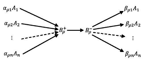
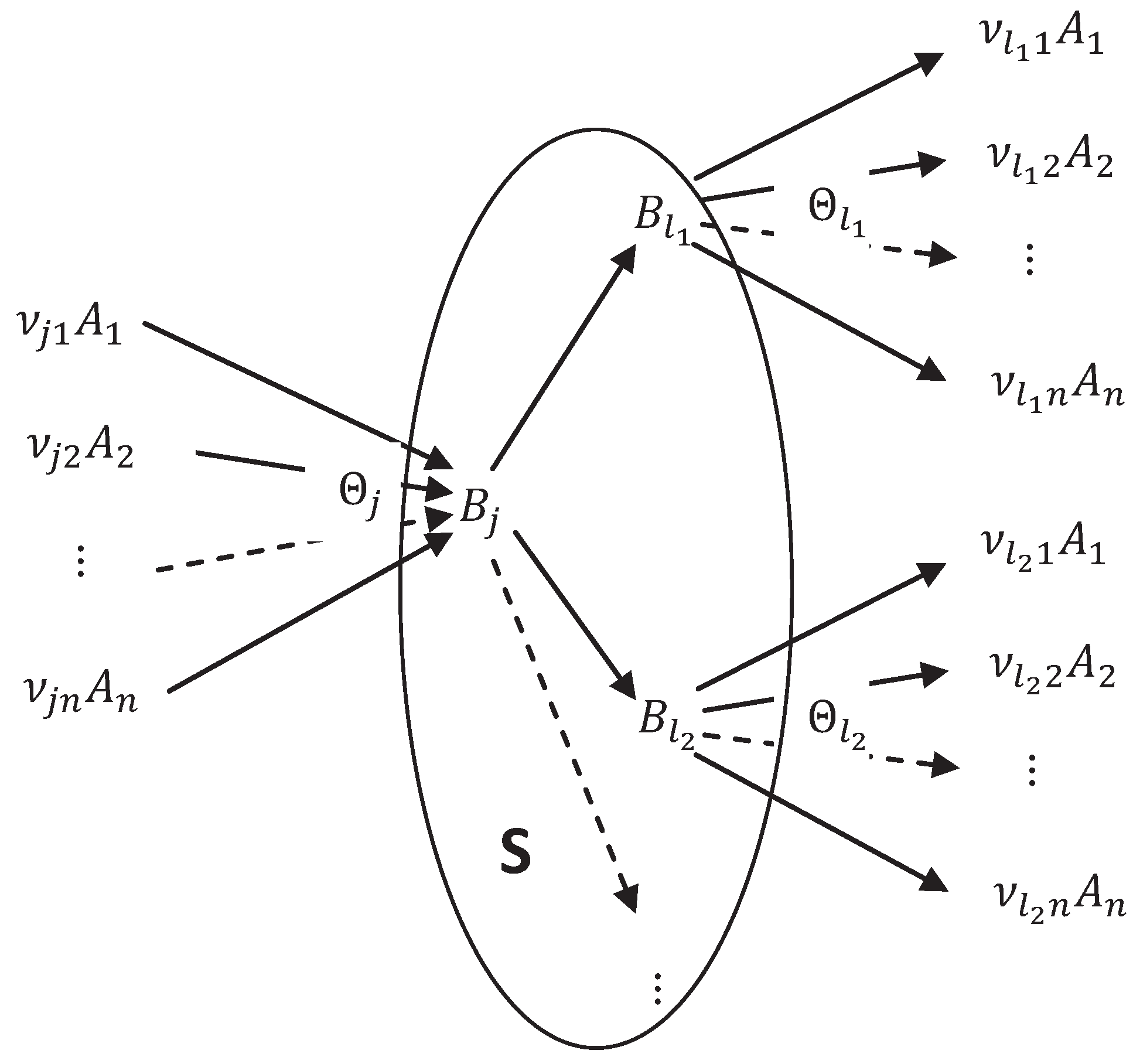
5.1. Stoichiometry of Complexes

In this Section, we return to the very general reaction network.

Let us call all the formal sums that participate in the stoichiometric equations (17), the complexes. The set of complexes for a given reaction mechanism (17) is ${\Theta }_1,\dots ,{\Theta }_q$. The number of complexes $q\le 2m$ (two complexes per elementary reaction, as the maximum) and it is possible that $q<2m$ because some complexes may coincide for different reactions.

A complex ${\Theta }_i$ is a formal sum ${\Theta }_i={\sum }_{j=1}^n{\nu }_{ij}{A}_j=({\nu }_i,A)$, where ${\nu }_i$ is a vector with coordinates ${\nu }_{ij}$.

Each elementary reaction (17) may be represented in the form ${\Theta }_{\rho }^{-}\to {\Theta }_{\rho }^{+}$, where ${\Theta }_{\rho }^{\pm }$ are the complexes which correspond to the right and the left sides (17). The whole mechanism is naturally represented as a digraph of transformation of complexes: Vertices are complexes and edges are reactions. This graph gives a convenient tool for the reaction representation and is often called the “reaction graph".

Let us consider a simple example: 18 elementary reactions (9 pairs of mutually reverse reactions) from the hydrogen combustion mechanism (see, for example, [48]).

$$\begin{array}{cc}\mathrm{H}+{\mathrm{O}}_2\rightleftharpoons \mathrm{O}+\mathrm{OH};\hfill & \mathrm{O}+{\mathrm{H}}_2\rightleftharpoons \mathrm{H}+\mathrm{OH};\hfill \\ \mathrm{OH}+{\mathrm{H}}_2\rightleftharpoons \mathrm{H}+{\mathrm{H}}_2\mathrm{O};\hfill & \mathrm{O}+{\mathrm{H}}_2\mathrm{O}\rightleftharpoons 2\mathrm{OH};\hfill \\ {\mathrm{HO}}_2+\mathrm{H}\rightleftharpoons {\mathrm{H}}_2+{\mathrm{O}}_2;\hfill & {\mathrm{HO}}_2+\mathrm{H}\rightleftharpoons 2\mathrm{OH};\hfill \\ \mathrm{H}+\mathrm{OH}+\mathrm{M}\rightleftharpoons {\mathrm{H}}_2\mathrm{O}+\mathrm{M};\hfill & \mathrm{H}+{\mathrm{O}}_2+\mathrm{M}\rightleftharpoons {\mathrm{HO}}_2+\mathrm{M};\hfill \\ {\mathrm{H}}_2{\mathrm{O}}_2+\mathrm{H}\rightleftharpoons {\mathrm{H}}_2+{\mathrm{HO}}_2\hfill \end{array}$$

(44)

There are 16 different complexes here:

$$\begin{array}{c}{\Theta }_1=\mathrm{H}+{\mathrm{O}}_2,{\Theta }_2=\mathrm{O}+\mathrm{OH},{\Theta }_3=\mathrm{O}+{\mathrm{H}}_2,{\Theta }_4=\mathrm{H}+\mathrm{OH},\hfill \\ {\Theta }_5=\mathrm{OH}+{\mathrm{H}}_2,{\Theta }_6=\mathrm{H}+{\mathrm{H}}_2\mathrm{O},{\Theta }_7=\mathrm{O}+{\mathrm{H}}_2\mathrm{O},{\Theta }_8=2\mathrm{OH},\hfill \\ {\Theta }_9={\mathrm{HO}}_2+\mathrm{H},{\Theta }_{10}={\mathrm{H}}_2+{\mathrm{O}}_2,{\Theta }_{11}=\mathrm{H}+\mathrm{OH}+\mathrm{M},\hfill \\ {\Theta }_{12}={\mathrm{H}}_2\mathrm{O}+\mathrm{M},{\Theta }_{13}=\mathrm{H}+{\mathrm{O}}_2+\mathrm{M},{\Theta }_{14}={\mathrm{HO}}_2+\mathrm{M},\hfill \\ {\Theta }_{15}={\mathrm{H}}_2{\mathrm{O}}_2+\mathrm{H},{\Theta }_{16}={\mathrm{H}}_2+{\mathrm{HO}}_2\hfill \end{array}$$

The reaction set (44) can be represented as

$$\begin{array}{c}{\Theta }_1\rightleftharpoons {\Theta }_2,{\Theta }_3\rightleftharpoons {\Theta }_4,{\Theta }_5\rightleftharpoons {\Theta }_6,{\Theta }_7\rightleftharpoons {\Theta }_8\rightleftharpoons {\Theta }_9\leftrightharpoons {\Theta }_{10},\hfill \\ {\Theta }_{11}\rightleftharpoons {\Theta }_{12},{\Theta }_{13}\rightleftharpoons {\Theta }_{14},{\Theta }_{15}\rightleftharpoons {\Theta }_{16}\hfill \end{array}$$

We can see that this digraph of transformation of complexes has a very simple structure: There are six isolated pairs of complexes and one connected group of four complexes.

5.2. Stoichiometry of Compounds

For each complex ${\Theta }_j$ we introduce an additional component $B_j$, an intermediate compound and $B_{\rho }^{\pm }$ are those compounds $B_j$ ($1\le j\le q$), which correspond to the right and left sides of reaction (17).

We call these components “compounds” following the English translation of the original Michaelis-Menten paper [8] and keep “complexes” for the formal linear combinations ${\Theta }_j$.

An extended reaction mechanism includes two types of reactions: Equilibration between a complex and its compound (q reactions, one for each complex)

$${\Theta }_j\rightleftharpoons B_j$$

(45)

and transformation of compounds $B_{\rho }^{-}\to B_{\rho }^{+}$ (m reactions, one for each elementary reaction from (17). So, instead of the reaction (17) we can write

$$\sum _i{\alpha }_{\rho i}{A}_i\rightleftharpoons B_{\rho }^{-}\to B_{\rho }^{+}\rightleftharpoons \sum _i{\beta }_{\rho i}{A}_i$$

(46)

Of course, if the input or output complexes coincide for two reactions then the corresponding equilibration reactions also coincide.

It is useful to visualize the reaction scheme. In Figure 1 we represent the $2n$-tail scheme of an elementary reaction sequence (46) which is an extension of the elementary reaction (17).

The reactions between compounds may have several channels (Figure 2): One complex may transform to several other complexes.

The reaction mechanism is a set of multichannel transformations (Figure 2) for all input complexes. In Figure 2 we grouped together the reactions with the same input complex. Another representation of the reaction mechanism is based on the grouping of reactions with the same output complex. Below, in the description of the complex balance condition, we use both representations.

The extended list of components includes $n+q$ components: n initial species $A_i$ and q compounds $B_j$. The corresponding composition vector $N^{\oplus }$ is a direct sum of two vectors, the composition vector for initial species, N, with coordinates $N_i$ ($i=1,\dots ,n$) and the composition vector for compounds, Υ, with coordinates ${{\rm Y}}_j$ ($j=1,\dots ,q$): $N^{\oplus }=N\oplus {\rm Y}$.

The space of composition vectors E is a direct sum of n-dimensional $E_A$ and q-dimensional $E_B$: $E=E_A\oplus E_B$.

For concentrations of $A_i$ we use the notation $c_i$ and for concentrations of $B_j$ we use ${\varsigma }_j$.

The stoichiometric vectors for reactions ${\Theta }_j\rightleftharpoons B_j$ (45) are direct sums: $g^j=-{\nu }_j\oplus e_j$, where $e_j$ is the jth standard basis vector of the space $R^q=E_B$, the coordinates of $e_j$ are $e_{jl}={\delta }_{jl}$:

$$g^j=(-{\nu }_{j1},-{\nu }_{j2},\dots ,-{\nu }_{jn},\underset{l}{\underbrace{0,\dots ,0,1}},0,\dots ,0)$$

(47)

The stoichiometric vectors of equilibration reactions (45) are linearly independent because there exists exactly one vector for each l.

The stoichiometric vectors ${\gamma }^{jl}$ of reactions $B_j\to B_l$ belong entirely to $E_B$. They have jth coordinate $-1$, lth coordinate $+1$ and other coordinates are zeros.

To exclude some degenerated cases a hypothesis of weak reversibility is accepted. Let us consider a digraph with vertices ${\Theta }_i$ and edges, which correspond to reactions from (17). The system is weakly reversible if for any two vertices ${\Theta }_i$ and ${\Theta }_j$, the existence of an oriented path from ${\Theta }_i$ to ${\Theta }_j$ implies the existence of an oriented path from ${\Theta }_j$ to ${\Theta }_i$.

Of course, this weak reversibility property is equivalent to weak reversibility of the reaction network between compounds $B_j$.

5.3. Energy, Entropy and Equilibria of Compounds

In this section, we define the free energy of the system. The basic hypothesis is that the compounds are the small admixtures to the system, that is, the amount of compounds $B_j$ is much smaller than amount of initial components $A_i$. Following this hypothesis, we neglect the energy of interaction between compounds, which is quadratic in their concentrations because in the low density limit we can neglect the correlations between particles if the potential of their interactions decay sufficiently fast when the distance between particles goes to ∞ [50]. We take the energy of their interaction with $A_i$ in the linear approximation, and use the perfect entropy for $B_i$. These standard assumptions for a small admixtures give for the free energy:

$$F=Vf(c,T)+VRT\sum _{j=1}^q{\varsigma }_j\left(\frac{u_j(c,T)}{RT}+ln{\varsigma }_j-1\right)$$

(48)

Let us introduce the standard equilibrium concentrations for $B_j$. Due to the Boltzmann distribution ($exp(-u/RT)$) and formula (48)

$${\varsigma }_j^{*}(c,T)=\frac{1}{Z}exp\left(-\frac{u_j(c,T)}{RT}\right)$$

(49)

where $1/Z$ is the normalization factor. Let us select here the normalization $Z=1$ and write:

$$F=Vf(c,T)+VRT\sum _{j=1}^q{\varsigma }_j\left(ln\left(\frac{{\varsigma }_j}{{\varsigma }_j^{*}(c,T)}\right)-1\right)$$

(50)

We assume that the standard equilibrium concentrations ${\varsigma }_j^{*}(c,T)$ are much smaller than the concentrations of $A_i$. It is always possible because functions $u_j$ are defined up to an additive constant.

The formula for free energy is necessary to define the fast equilibria (45). Such an equilibrium is the minimizer of the free energy on the straight line parameterized by a: $c_i=c_i^0-a{\nu }_{ji}$, ${\varsigma }_j=a$.

If we neglect the products ${\varsigma }_j\partial {\varsigma }_j^{*}(c,T)/\partial c_i$ as the second order small quantities then the minimizers have the very simple form:

$${\vartheta }_j=\sum _i{\nu }_{ji}\frac{{\mu }_i(c,T)}{RT}$$

(51)

or

$${\varsigma }_j={\varsigma }_j^{*}(c,T)exp\left(\frac{{\sum }_i{\nu }_{ji}{\mu }_i(c,T)}{RT}\right)$$

(52)

where

$${\mu }_i=\frac{\partial f(c,T)}{\partial c_i}$$

is the chemical potential of $A_i$ and

$${\vartheta }_j=ln\left(\frac{{\varsigma }_j}{{\varsigma }_j^{*}}\right)$$

($RT{\vartheta }_j=\frac{1}{V}\frac{\partial F}{\partial {\varsigma }_j}$ is the chemical potential of $B_j$).

The thermodynamic equilibrium of the system of reactions $B_j\to B_l$ that corresponds to the reactions (46) is the free energy minimizer under given values of the conservation laws.

For the systems with fixed volume, the stoichiometric conservation laws of the monomolecular system of reaction are sums of the concentrations of $B_j$ which belong to the connected components of the reaction graph. Under the hypothesis of weak reversibility there is no other conservation law. Let the graph of reactions $B_j\to B_l$ have d connected components $C_s$ and let $V_s$ be the set of indexes of those $B_j$ which belong to $C_s$: $B_j\in C_s$ if and only if $j\in V_s$. For each $C_s$ there exists a stoichiometric conservation law

$${\beta }_s=\sum _{j\in V_s}{\varsigma }_j=const$$

(53)

For any set of positive values of ${\beta }_s$ ($s=1,\dots ,d$) and given $c,T$ there exists a unique conditional maximizer ${\varsigma }_j^{\mathrm{eq}}$ of the free energy (50): For the compound $B_j$ from the sth connected component ($j\in V_s$) this equilibrium concentration is

$${\varsigma }_j^{\mathrm{eq}}={\beta }_s\frac{{\varsigma }_j^{*}(c,T)}{{\sum }_{l\in V_s}{\varsigma }_j^{*}(c,T)}$$

(54)

The positive values of concentrations ${\varsigma }_j$ are the equilibrium concentrations (54) for some values of ${\beta }_s$ if and only if for any $s=1,\dots ,d$ and all $j,l\in V_s$

$${\vartheta }_j={\vartheta }_l$$

(55)

(${\vartheta }_j=ln({\varsigma }_j/{\varsigma }_j^{*})$). This means that compounds are in equilibrium in every connected component $C_s$ the chemical potentials of compounds coincide in each component $C_s$. The system of equations (55) together with the equilibrium conditions (52) constitute the equilibrium of the systems. All the equilibria form a linear subspace in the space with coordinates ${\mu }_i/RT$ ($i=1,\dots ,n$) and ${\vartheta }_j$ ($j=1,\dots ,q$).

In the expression for the free energy (50) we do not assume anything special about free energy of the mixture of $A_i$. The density of this free energy, $f(c,T)$, may be an arbitrary smooth function (later, we will add the standard assumption about convexity of $f(c,T)$ as a function of c). For the compounds $B_i$, we assume that they form a very small addition to the mixture of $A_i$, neglect all quadratic terms in concentrations of $B_i$ and use the entropy of the perfect systems, $plnp$, for this small admixture.

This approach results in the explicit expressions for the fast equilibria (52) and expression of the equilibrium compound concentrations through the values of the stoichiometric conservation laws (54).

5.4. Markov Kinetics of Compounds

For the kinetics of compounds transformations $B_j\to B_l$, the same hypothesis of the smallness of concentrations leads to the only reasonable assumption: The linear (monomolecular) kinetics with the rate constant ${\kappa }_{lj}>0$. This “constant” is a function of $c,T$: ${\kappa }_{lj}(c,T)$. The order of indexes at κ is inverse to the order of them in reaction: ${\kappa }_{lj}={\kappa }_{l\leftarrow j}$.

The master equation for the concentration of $B_j$ gives:

$$\frac{\mathrm{d}{\varsigma }_j}{\mathrm{d}t}=\sum _{l,l\ne j}\left({\kappa }_{jl}{\varsigma }_l-{\kappa }_{lj}{\varsigma }_j\right)$$

(56)

It is necessary to find when this kinetics respect thermodynamics, i.e., when the free energy decreases due to the system (56). The necessary and sufficient condition for matching the kinetics and thermodynamics is: The standard equilibrium ${\varsigma }^{*}$ (49) should be an equilibrium for (56), that is, for every $j=1,\dots ,q$

$$\sum _{l,l\ne j}{\kappa }_{jl}{\varsigma }_l^{*}=\sum _{l,l\ne j}{\kappa }_{lj}{\varsigma }_j^{*}$$

(57)

This condition is necessary because the standard equilibrium is the free energy minimizer for given $c,T$ and ${\sum }_j{\varsigma }_j={\sum }_j{\varsigma }_j^{*}$. The sum ${\sum }_j{\varsigma }_j$ conserves due to (56). Therefore, if we assume that F decreases monotonically due to (56) then the point of conditional minimum of F on the plane ${\sum }_j{\varsigma }_j=const$ (under given $c,T$) should be an equilibrium point for this kinetic system. This condition is sufficient due to the Morimoto H-theorem (see Appendix 2).

For a weakly reversible system, the set of the conditional minimizers of the free energy (54) coincides with with the set of positive equilibria for the master equations (56) (see Equation (132) in Appendix 2).

5.5. Thermodynamics and Kinetics of the Extended System

In this section, we consider the complete extended system, which consists of species $A_i$ ($i=1,\dots ,n$) and compounds $B_j$ ($j=1,\dots ,q$) and includes reaction of equilibration (45) and transformations of compounds $B_j\to B_l$ which correspond to the reactions (46).

Thermodynamic properties of the system are summarized in the free energy function (50). For kinetics of compounds we accept the Markov model (56) with the equilibrium condition (57), which guarantees matching between thermodynamics and kinetics.

For the equilibration reactions (45) we select a very general form of the kinetic law. The only requirement is: This reaction should go to its equilibrium, which is described as the conditional minimizer of free energy F (52). For each reaction ${\Theta }_j\rightleftharpoons B_j$ (where the complex is a formal combination: ${\Theta }_j={\sum }_i{\nu }_{ji}{A}_i$) we introduce the reaction rate $w_j$. This rate should be positive if

$${\vartheta }_j<\sum _i{\nu }_{ji}\frac{{\mu }_i(c,T)}{RT}$$

(58)

and negative if

$${\vartheta }_j>\sum _i{\nu }_{ji}\frac{{\mu }_i(c,T)}{RT}$$

(59)

The general way to satisfy these requirement is to select q continuous function of real variable $w_j\left(x\right)$, which are negative if $x>0$ and positive if $x<0$. For the equilibration rates we take

$$w_j=w_j\left({\vartheta }_j-\sum _i{\nu }_{ji}\frac{{\mu }_i(c,T)}{RT}\right)$$

(60)

If several dynamical systems defined by equations $\dot{x}=J_1$, ... $\dot{x}=J_v$ on the same space have the same Lyapunov function F, then for any conic combination $J={\sum }_k{a}_k{J}_k$ ($a_k\ge 0$, ${\sum }_k{a}_k>0$) the dynamical system $\dot{x}=J$ also has the Lyapunov function F.

The free energy (50) decreases monotonically due to any reaction ${\Theta }_j\rightleftharpoons B_j$ with reaction rate $w_j$ (60) and also due to the Markov kinetics (56) with the equilibrium condition (57). Therefore, the free energy decreases monotonically due to the following kinetic system:

$$\begin{array}{c}\frac{\mathrm{d}{c}_i}{\mathrm{d}t}=-\sum _{j=1}^q{\nu }_{ji}{w}_j\hfill \\ \frac{\mathrm{d}{\varsigma }_j}{\mathrm{d}t}=w_j+\sum _{l,l\ne j}\left({\kappa }_{jl}{\varsigma }_l-{\kappa }_{lj}{\varsigma }_j\right)\hfill \end{array}$$

(61)

where the coefficients ${\kappa }_{jl}$ satisfy the matching condition (57).

This general system (61) describes kinetics of extended system and satisfies all the basic conditions (thermodynamics and smallness of compound concentrations). In the next sections we will study the QE approximations to this system and exclude the unknown functions $w_j$ from it.

5.6. QE Elimination of Compounds and the Complex Balance Condition

In this section, we use the QE formalism developed for chemical kinetics in Section 4 for simplification of the compound kinetics.

First of all, let us describe $L^{\perp }$, where the space L is the subspace in the extended concentration space spanned by the stoichiometric vectors of fast equilibration reactions (45). The stoichiometric vector for the equilibration reactions have a very special structure (47). Dimension of the space L is equal to the number of complexes: $dimL=q$. Therefore, dimension of $L^{\perp }$ is equal to the number of components $A_i$: $dim{L}^{\perp }=n$. For each $A_i$ we will find a vector $b_i\in L^{\perp }$ that has the following first n coordinates: $b_{ik}={\delta }_{ik}$ for $k=1,\dots ,n$. The condition $(b_i,g_j)=0$ gives immediately: $b_{i,n+j}={\nu }_{ji}$. Finally,

$$b_i=(\stackrel{n}{\overbrace{\underset{i}{\underbrace{0,\dots ,0,1}},0,\dots ,0}},{\nu }_{1i},{\nu }_{2i},\dots ,{\nu }_{qi})$$

(62)

The corresponding slow variables are

$$b_i(c,\varsigma )=c_i+\sum _j{\varsigma }_j{\nu }_{ji}$$

(63)

In the QE approximation all $w_j=0$ and the kinetic equations (61) give in this approximation

$$\frac{\mathrm{d}{b}_i}{\mathrm{d}t}=\sum _{lj,l\ne j}({\kappa }_{jl}{\varsigma }_l-{\kappa }_{lj}{\varsigma }_j){\nu }_{ji}$$

(64)

In these equations, we have to use the dependence $\varsigma \left(b\right)$. Here we use the QSS Michaelis and Menten assumption: The compounds are present in small amounts

$$c_i\gg {\varsigma }_j$$

In this case, we can take $b_i$ instead of $c_i$ (i.e., take $\mu (b,T)$ instead of $\mu (c,T)$) in the formulas for equilibria (52):

$${\varsigma }_j={\varsigma }_j^{*}(b,T)exp\left(\frac{{\sum }_i{\nu }_{ji}{\mu }_i(b,T)}{RT}\right)$$

(65)

In the final form of the QE kinetic equation there remain two “offprints” of the compound kinetics: Two sets of functions ${\varsigma }_j^{*}(b,T)\ge 0$ and ${\kappa }_{jl}(b,T)\ge 0$. These functions are connected by the identity (57). The final form of the equations is

$$\begin{array}{cc}\hfill \frac{\mathrm{d}{b}_i}{\mathrm{d}t}=& \sum _{lj,l\ne j}\left({\kappa }_{jl}{\varsigma }_l^{*}(b,T)exp\left(\frac{{\sum }_i{\nu }_{li}{\mu }_i(b,T)}{RT}\right)-{\kappa }_{lj}{\varsigma }_j^{*}(b,T)exp\left(\frac{{\sum }_i{\nu }_{ji}{\mu }_i(b,T)}{RT}\right)\right){\nu }_{ji}\hfill \end{array}$$

(66)

The identity (57), ${\sum }_{l,l\ne j}{\kappa }_{jl}{\varsigma }_l^{*}={\sum }_{l,l\ne j}{\kappa }_{lj}{\varsigma }_j^{*}$, provides a sufficient condition for decreasing of free energy due to the kinetic equations(66). This is a direct consequence of two theorem: The theorem about the preservation of entropy production in the QE approximations (see Section 2 and Appendix 1) and the Morimoto H-theorem (see Appendix 2). Indeed, in the QE state the equilibrated reactions (45) ${\Theta }_j\rightleftharpoons B_j$ do not produce entropy and all changes in the total free energy are caused by the Markov kinetics $B_i\to B_j$. Due to the Morimoto H-theorem this change is negative: The Markov kinetics decrease the perfect free energy of compounds and do not affect the free energy of $A_i$. In the QE approximation, the concentrations of $A_i$ are changing together with concentrations of $B_j$ because of the equilibrium conditions for reactions ${\Theta }_j\rightleftharpoons B_j$. Due to the theorem of preservation of the entropy production, the time derivative of the total free energy in this QE dynamics coincides with the time derivative of the free energy of $B_j$ due to Markov kinetics. In addition to this proof, in Section 6 below we give the explicit formula for entropy production in (66) and direct proof of its positivity.

Let us stress that the functions ${\varsigma }_j^{*}(b,T)$ and ${\kappa }_{jl}(b,T)$ participate in equations (66) and in identity (57) in the form of the product. Below we use for this product a special notation:

$${\phi }_{jl}(b,T)={\kappa }_{jl}(b,T){\varsigma }_l^{*}(b,T)(j\ne l)$$

(67)

We call this function ${\phi }_{jl}(b,T)$ the kinetic factor. The identity (57) for the kinetic factor is

$$\sum _{l,l\ne j}{\phi }_{jl}(b,T)=\sum _{l,l\ne j}{\phi }_{lj}(b,T) \mathrm{for} \mathrm{all} j$$

(68)

We call the thermodynamic factor (or the Boltzmann factor) the second multiplier in the reaction rates

$${\Omega }_l(b,T)=exp\left(\frac{{\sum }_i{\nu }_{li}{\mu }_i(b,T)}{RT}\right)$$

(69)

In this notation, the kinetic equations (66) have a simple form

$$\frac{\mathrm{d}{b}_i}{\mathrm{d}t}=\sum _{lj,l\ne j}({\phi }_{jl}(b,T){\Omega }_l(b,T)-{\phi }_{lj}(b,T){\Omega }_j(b,T)){\nu }_{ji}$$

(70)

The general equations (70) have the form of “sum over complexes”. Let us return to the more usual “sum over reactions” form. An elementary reaction corresponds to the pair of complexes ${\Theta }_l,{\Theta }_j$ (46). It has the form ${\Theta }_l\to {\Theta }_j$ and the reaction rate is $r={\phi }_{jl}{\Omega }_l$. In the right hand side in (70) this reaction appears twice: first time with sign “+” and the vector coefficient ${\nu }_j$ and the second time with sign “−” and the vector coefficient ${\nu }_l$. The stoichiometric vector of this reaction is $\gamma ={\nu }_j-{\nu }_l$. Let us enumerate the elementary reactions by index ρ, which corresponds to the pair $(j,l)$. Finally, we transform (46) into the sum over reactions form

$$\begin{array}{cc}\hfill \frac{\mathrm{d}{b}_i}{\mathrm{d}t}& =\sum _{l,j,l\ne j}{\phi }_{jl}(b,T){\Omega }_l(b,T)({\nu }_{ji}-{\nu }_{li})\hfill \\ & =\sum _{\rho }{\phi }_{\rho }(b,T){\Omega }_{\rho }(b,T){\gamma }_{\rho i}\hfill \end{array}$$

(71)

In the vector form it looks as follows:

$$\frac{\mathrm{d}b}{\mathrm{d}t}=\sum _{\rho }{\phi }_{\rho }(b,T){\Omega }_{\rho }(b,T){\gamma }_{\rho }$$

(72)

5.7. The Big Michaelis-Menten-Stueckelberg Theorem

Let us summarize the results of our analysis in one statement.

Let us consider the reaction mechanism illustrated by Figure 2 (46):

$$\sum _i{\alpha }_{\rho i}{A}_i\rightleftharpoons B_{\rho }^{-}\to B_{\rho }^{+}\rightleftharpoons \sum _i{\beta }_{\rho i}{A}_i$$

under the following asymptotic assumptions:

• Concentrations of the compounds $B_{\rho }$ are close to their quasiequilibrium values (65)

  $${\varsigma }_j=(1+\delta ){\varsigma }_j^{\mathrm{QE}}=(1+\delta ){\varsigma }_j^{*}(b,T)exp\left(\frac{{\sum }_i{\nu }_{ji}{\mu }_i(b,T)}{RT}\right),\delta \ll 1$$

  (this may be due to the fast reversible reactions in (46));
• Concentrations of the compounds $B_{\rho }$ are much smaller than the concentrations of the components $A_i$: There is a small positive parameter $\epsilon \ll 1$, ${\varsigma }_j^{*}=\epsilon {\xi }_j^{*}$ and ${\xi }_j^{*}$ do not depend on ε;
• Kinetics of transitions between compounds $B_i\to B_j$ is linear (Markov) kinetics with reaction rate constants $k_{ji}=\frac{1}{\epsilon }{\kappa }_{ji}$.

Under these assumptions, in the asymptotic $\delta ,\epsilon \to 0$, $\delta ,\epsilon >0$ kinetics of components $A_i$ may be described by the reaction mechanism

$$\sum _i{\alpha }_{\rho i}{A}_i\to \sum _i{\beta }_{\rho i}{A}_i$$

with the reaction rates

$$r_{\rho }={\phi }_{\rho }exp\left(\frac{({\alpha }_{\rho },\mu )}{RT}\right)$$

where the kinetic factors ${\phi }_{\rho }$ satisfy the condition (68):

$$\sum _{\rho ,{\alpha }_{\rho }=\mathrm{v}}{\phi }_{\rho }\equiv \sum _{\rho ,{\beta }_{\rho }=\mathrm{v}}{\phi }_{\rho }$$

for any vector $\mathrm{v}$ from the set of all vectors $\{{\alpha }_{\rho },{\beta }_{\rho }\}$. This statement includes the generalized mass action law for $r_{\rho }$ and the balance identity for kinetic factors that is sufficient for the entropy growth as it is shown in the next Section 6.

6. General Kinetics and Thermodynamics

6.1. General Formalism

To produce the general kinetic law and the complex balance conditions, we use “construction staging”: The intermediate complexes with fast equilibria, the Markov kinetics and other important and interesting physical and chemical hypothesis.

In this section, we delete these construction staging and start from the forms (69), (72) as the basic laws. We use also the complex balance conditions (68) as a hint for the general conditions which guarantee accordance between kinetics and thermodynamics.

Let us consider a domain U in n-dimensional real vector space E with coordinates $N_1,\dots ,N_n$. For each $N_i$ a symbol (component) $A_i$ is given. A dimensionless entropy (or free entropy, for example, Massieu, Planck, or Massieu-Planck potential which correspond to the selected conditions [52]) $S\left(N\right)$ is defined in U. “Dimensionless” means that we use $S/R$ instead of physical S. This choice of units corresponds to the informational entropy ($plnp$ instead of $k_{\mathrm{B}}plnp$).

The dual variables, potentials, are defined as the partial derivatives of S:

$${\check{\mu }}_i=-\frac{\partial S}{\partial N_i}$$

(73)

Warning: This definition differs from the chemical potentials (22) by the factor $1/RT$: For constant volume the Massieu-Planck potential is $-F/T$ and we, in addition, divide it on R. On the other hand, we keep the same sign as for the chemical potentials, and this differs from the standard Legendre transform for S. (It is the Legendre transform for function $-S$).

The reaction mechanism is defined by the stoichiometric equations (17)

$$\sum _i{\alpha }_{\rho i}{A}_i\to \sum _i{\beta }_{\rho i}{A}_i$$

($\rho =1,\dots ,m$). In general, there is no need to assume that the stoichiometric coefficients ${\alpha }_{\rho i},{\beta }_{\rho i}$ are integers.

The assumption that they are nonnegative, ${\alpha }_{\rho i}\ge 0,{\beta }_{\rho i}\ge 0$, may be needed to prove that the kinetic equations preserve positivity of $N_i$. If $N_i$ is the number of particles then it is a natural assumption but we can use other extensive variables instead, for example, we included energy in the list of variables to describe the non-isothermal processes [53]. In this case, the coefficient ${\alpha }_U$ for the energy component $A_U$ in an exothermic reaction is negative.

So, for variables that are positive (bounded from below) by their physical sense, we will use the inequalities ${\alpha }_{\rho i}\ge 0,{\beta }_{\rho i}\ge 0$, when necessary, but in general, for arbitrary extensive variables, we do not assume positivity of stoichiometric coefficients. As it is usually, the stoichiometric vector of reaction is ${\gamma }_{\rho }={\beta }_{\rho }-{\alpha }_{\rho }$ (the “gain minus loss” vector).

For each reaction, a nonnegative quantity, reaction rate $r_{\rho }$ is defined. We assume that this quantity has the following structure:

$$r_{\rho }={\phi }_{\rho }exp({\alpha }_{\rho },\check{\mu })$$

(74)

where $({\alpha }_{\rho },\check{\mu })={\sum }_i{\alpha }_{\rho i}{\check{\mu }}_i$.

In the standard formalism of chemical kinetics the reaction rates are intensive variables and in kinetic equations for N an additional factor—the volume—appears. For heterogeneous systems, there may be several “volumes” (including interphase surfaces).

Each reaction has it own “volume”, an extensive variable $V_{\rho }$ (some of them usually coincide), and we can write

$$\frac{\mathrm{d}N}{\mathrm{d}t}=\sum _{\rho }{V}_{\rho }{\gamma }_{\rho }{\phi }_{\rho }exp({\alpha }_{\rho },\check{\mu })$$

(75)

In these notations, both the kinetic and the Boltzmann factors are intensive (and local) characteristics of the system.

Let us, for simplicity of notations, consider a system with one volume, V and write

$$\frac{\mathrm{d}N}{\mathrm{d}t}=V\sum _{\rho }{\gamma }_{\rho }{\phi }_{\rho }exp({\alpha }_{\rho },\check{\mu })$$

(76)

Below we use the form (76). All our results will hold also for the multi-volume systems (75) under one important assumption: The elementary reaction

$$\sum _i{\alpha }_{\rho i}{A}_i\to \sum _i{\beta }_{\rho i}{A}_i$$

goes in the same volume as the reverse reaction

$$\sum _i{\beta }_{\rho i}{A}_i\to \sum _i{\alpha }_{\rho i}{A}_i$$

or symbolically

$$V_{\rho }^{+}=V_{\rho }^{-}$$

(77)

If this condition (77) holds then the detailed balance conditions and the complex balance conditions will hold separately in all volumes $V_{\rho }$.

An important particular case of (76) gives us the Mass Action Law. Let us take the perfect free entropy

$$S=-\sum _i{N}_i\left(ln\left(\frac{c_i}{c_i^{*}}\right)-1\right)$$

(78)

where $c_i=N_i/V\ge 0$ are concentrations and $c_i^{*}>0$ are the standard equilibrium concentrations. Under isochoric conditions, $V=const$, there is no difference between the choice of the main variables, N or c.

For the perfect function (78)

$${\check{\mu }}_i=ln\left(\frac{c_i}{c_i^{*}}\right),exp({\alpha }_{\rho },\check{\mu })=\prod _i{\left(\frac{c_i}{c_i^{*}}\right)}^{{\alpha }_{\rho i}}$$

(79)

and for the reaction rate function (74) we get

$$r_{\rho }={\phi }_{\rho }\prod _i{\left(\frac{c_i}{c_i^{*}}\right)}^{{\alpha }_{\rho i}}$$

(80)

The standard assumption for the Mass Action Law in physics and chemistry is that ϕ and $c^{*}$ are functions of temperature: ${\phi }_{\rho }={\phi }_{\rho }\left(T\right)$ and $c_i^{*}=c_i^{*}\left(T\right)$. To return to the kinetic constants notation (20) we should write:

$$\frac{{\phi }_{\rho }}{{\prod }_i{c_i^{*}}^{{\alpha }_{\rho i}}}=k_{\rho }$$

Equation (76) is the general form of the kinetic equation we would like to study. In many senses, this form is too general before we impose restrictions on the values of the kinetic factors. For physical and chemical systems, thermodynamics is a source of restrictions:

• The energy of the Universe is constant.
• The entropy of the Universe tends to a maximum.

(R. Clausius, 1865 [54].)

The first sentence should be extended: The kinetic equations should respect several conservation laws: Energy, amount of atoms of each kind (if there is no nuclear reactions in the system) conservation of total probability and, sometimes, some other conservation laws. All of them have the form of conservation of values of some linear functionals: $l\left(N\right)=const$. If the input and output flows are added to the system then

$$\frac{\mathrm{d}l\left(N\right)}{\mathrm{d}t}=V{v}^{\mathrm{in}}{l}^{\mathrm{in}}-v^{\mathrm{out}}l\left(N\right)$$

where $v^{\mathrm{in},\mathrm{out}}$ are the input and output fluxes per unit volume, $l^{\mathrm{in}}$ are the input densities (concentration). The standard requirement is that every reaction respects all these conservation laws. The formal expression of this requirement is:

$$l\left({\gamma }_{\rho }\right)=0 \mathrm{for} \mathrm{all} \rho$$

(81)

There is a special term for this conservation laws: The stoichiometric conservation laws. All the main conservation laws are assumed to be the stoichiometric ones.

Analysis of the stoichiometric conservation laws is a simple linear algebra task: We have to find the linear functionals that annulate all the stoichiometric vectors ${\gamma }_{\rho }$. In contrast, entropy is not a linear function of N and analysis of entropy production is not so simple.

In the next subsection we discuss various conditions which guarantee the positivity of entropy production in kinetic equations (76).

6.2. Accordance Between Kinetics and Thermodynamics

6.2.1. General Entropy Production Formula

Let us calculate $\mathrm{d}S/\mathrm{d}t$ due to equations (76):

$$\begin{array}{cc}\hfill \frac{\mathrm{d}S}{\mathrm{d}t}& =\sum _i\frac{\partial S}{\partial N_i}\frac{\mathrm{d}{N}_i}{\mathrm{d}t}\hfill \\ & =-\sum _i{\check{\mu }}_{i}V\sum _{\rho }{\gamma }_{\rho i}{\phi }_{\rho }exp({\alpha }_{\rho },\check{\mu })\hfill \\ & =-V\sum _{\rho }({\gamma }_{\rho },\check{\mu }){\phi }_{\rho }exp({\alpha }_{\rho },\check{\mu })\hfill \end{array}$$

(82)

An auxiliary function $\theta \left(\lambda \right)$ of one variable $\lambda \in [0,1]$ is convenient for analysis of $\mathrm{d}S/\mathrm{d}t$ (it was studied by Rozonoer and Orlov [55], see also [25]:

$$\theta \left(\lambda \right)=\sum _{\rho }{\phi }_{\rho }exp\left[(\check{\mu },(\lambda {\alpha }_{\rho }+(1-\lambda ){\beta }_{\rho }))\right]$$

(83)

With this function, the entropy production (82) has a very simple form:

$$\frac{\mathrm{d}S}{\mathrm{d}t}=V{\left.\frac{\mathrm{d}\theta \left(\lambda \right)}{\mathrm{d}\lambda }\right|}_{\lambda =1}$$

(84)

The auxiliary function $\theta \left(\lambda \right)$ allows the following interpretation. Let us introduce the deformed stoichiometric mechanism with the stoichiometric vectors,

$${\alpha }_{\rho }\left(\lambda \right)=\lambda {\alpha }_{\rho }+(1-\lambda ){\beta }_{\rho },{\beta }_{\rho }\left(\lambda \right)=\lambda {\beta }_{\rho }+(1-\lambda ){\alpha }_{\rho }$$

which is the initial mechanism when $\lambda =1$, the inverted mechanism with interchange of α and β when $\lambda =0$, the trivial mechanism (the left and right hand sides of the stoichiometric equations coincide) when $\lambda =1/2$.

For the deformed mechanism, let us take the same kinetic factors and calculate the Boltzmann factors with ${\alpha }_{\rho }\left(\lambda \right)$:

$$r_{\rho }\left(\lambda \right)={\phi }_{\rho }exp({\alpha }_{\rho }\left(\lambda \right),\check{\mu })$$

In this notation, the auxiliary function $\theta \left(\lambda \right)$ is a sum of reaction rates for the deformed reaction mechanism:

$$\theta \left(\lambda \right)=\sum _{\rho }{r}_{\rho }\left(\lambda \right)$$

In particular, $\theta \left(1\right)={\sum }_{\rho }{r}_{\rho }$, this is just the sum of reaction rates.

Function $\theta \left(\lambda \right)$ is convex. Indeed

$$\frac{{\mathrm{d}}^2\theta \left(\lambda \right)}{\mathrm{d}{\lambda }^2}=\sum _{\rho }{\phi }_{\rho }{({\gamma }_{\rho },\check{\mu })}^{2}exp\left[(\check{\mu },(\lambda {\alpha }_{\rho }+(1-\lambda ){\beta }_{\rho }))\right]\ge 0$$

This convexity gives the following necessary and sufficient condition for positivity of entropy production:

$$\frac{\mathrm{d}S}{\mathrm{d}t}>0 \mathrm{if} \mathrm{and} \mathrm{only} \mathrm{if} \theta \left(\lambda \right)<\theta \left(1\right) \mathrm{for} \mathrm{some} \lambda <1$$

In several next subsections we study various important particular sufficient conditions for positivity of entropy production.

6.2.2. Detailed Balance

The most celebrated condition which gives the positivity of entropy production is the principle of detailed balance. Boltzmann used this principle to prove his famous H-theorem [27].

Let us join elementary reactions in pairs:

$$\sum _i{\alpha }_{\rho i}{A}_i\rightleftharpoons \sum _i{\beta }_{\rho i}{A}_i$$

(85)

After this joining, the total amount of stoichiometric equations decreases. If there is no reverse reaction then we can add it formally, with zero kinetic factor. We will distinguish the reaction rates and kinetic factors for direct and inverse reactions by the upper plus or minus:

$$r_{\rho }^{+}={\phi }_{\rho }^{+}exp({\alpha }_{\rho },\check{\mu }),r_{\rho }^{-}={\phi }_{\rho }^{-}exp({\beta }_{\rho },\check{\mu }),r_{\rho }=r_{\rho }^{+}-r_{\rho }^{-}$$

$$\frac{\mathrm{d}N}{\mathrm{d}t}=V\sum _{\rho }{\gamma }_{\rho }{r}_{\rho }$$

(86)

In this notation, the principle of detailed balance is very simple: The thermodynamic equilibrium in the direction ${\gamma }_{\rho }$, given by the standard condition $({\gamma }_{\rho },\check{\mu })=0$, is equilibrium for the corresponding pair of mutually reverse reactions from (85). For kinetic factors this transforms into the simple and beautiful condition:

$${\phi }_{\rho }^{+}exp({\alpha }_{\rho },\check{\mu })={\phi }_{\rho }^{-}exp({\beta }_{\rho },\check{\mu })\iff ({\gamma }_{\rho },\check{\mu })=0$$

therefore

$${\phi }_{\rho }^{+}={\phi }_{\rho }^{-}$$

(87)

For the systems with detailed balance we can take ${\phi }_{\rho }={\phi }_{\rho }^{+}={\phi }_{\rho }^{-}$ and write for the reaction rate:

$$r_{\rho }={\phi }_{\rho }(exp({\alpha }_{\rho },\check{\mu })-exp({\beta }_{\rho },\check{\mu }))$$

M. Feinberg called this kinetic law the “Marselin-De Donder” kinetics [46]. This representation of the reaction rates gives for the auxiliary function $\theta \left(\lambda \right)$:

$$\theta \left(\lambda \right)=\sum _{\rho }{\phi }_{\rho }(exp\left[(\check{\mu },(\lambda {\alpha }_{\rho }+(1-\lambda ){\beta }_{\rho }))\right]+exp\left[(\check{\mu },(\lambda {\beta }_{\rho }+(1-\lambda ){\alpha }_{\rho }))\right])$$

(88)

Each term in this sum is symmetric with respect to change $\lambda \mapsto (1-\lambda )$. Therefore, $\theta \left(1\right)=\theta \left(0\right)$ and, because of convexity of $\theta \left(\lambda \right)$, ${\theta }^{\prime }\left(1\right)\ge 0$. This means positivity of entropy production.

The principle of detailed balance is a sufficient but not a necessary condition of the positivity of entropy production. This was clearly explained, for example, by L. Onsager [56,57]. Interrelations between positivity of entropy production, Onsager reciprocal relations and detailed balance were analyzed in detail by N.G. van Kampen [58].

6.2.3. Complex Balance

The principle of detailed balance gives us $\theta \left(1\right)=\theta \left(0\right)$ and this equality holds for each pair of mutually reverse reactions.

Let us start now from the equality $\theta \left(1\right)=\theta \left(0\right)$. We return to the initial stoichiometric equations (17) without joining the direct and reverse reactions. The equality reads

$$\sum _{\rho }{\phi }_{\rho }exp(\check{\mu },{\alpha }_{\rho })=\sum _{\rho }{\phi }_{\rho }exp(\check{\mu },{\beta }_{\rho })$$

(89)

Exponential functions $exp(\check{\mu },y)$ form linearly independent family in the space of functions of $\check{\mu }$ for any finite set of pairwise different vectors y. Therefore, the following approach is natural: Let us equalize in (89) the terms with the same Boltzmann-type factor $exp(\check{\mu },y)$. Here we have to return to the complex-based representation of reactions (see Section 5.1).

Let us consider the family of vectors $\{{\alpha }_{\rho },{\beta }_{\rho }\}$ ($\rho =1,\dots ,m$). Usually, some of these vectors coincide. Assume that there are q different vectors among them. Let $y_1,\dots ,y_q$ be these vectors. For each $j=1,\dots ,q$ we take

$$R_j^{+}=\left\{\rho \right|{\alpha }_{\rho }=y_j\},R_j^{-}=\left\{\rho \right|{\beta }_{\rho }=y_j\}$$

We can rewrite the equality (89) in the form

$$\sum _{j=1}^{q}exp(\check{\mu },y_j)\left[\sum _{\rho \in R_j^{+}}{\phi }_{\rho }-\sum _{\rho \in R_j^{-}}{\phi }_{\rho }\right]=0$$

(90)

The Boltzmann factors $exp(\check{\mu },y_j)$ form the linearly independent set. Therefore the natural way to meet these condition is: For any $j=1,\dots ,q$

$$\sum _{\rho \in R_j^{+}}{\phi }_{\rho }-\sum _{\rho \in R_j^{-}}{\phi }_{\rho }=0$$

(91)

This is the general complex balance condition. This condition is sufficient for entropy growth, because it provides the equality $\theta \left(1\right)=\theta \left(0\right)$.

If we assume that ${\phi }_{\rho }$ are constants or, for chemical kinetics, depend only on temperature, then the conditions (91) give the general solution to equation (90).

The complex balance condition is more general than the detailed balance. Indeed, this is obvious: For the master equation (56) the complex balance condition is trivially valid for all admissible constants. The first order kinetics always satisfies the complex balance conditions. On the contrary, the class of the master equations with detailed balance is rather special. The dimension of the class of all master equations has dimension $n^2-n$ (constants for all transitions $A_i\to A_j$ are independent). For the time-reversible Markov chains (the master equations with detailed balance) there is only $n(n+1)/2-1$ independent constants: $n-1$ for equilibrium state and $n(n-1)/2$ for transitions $A_i\to A_j$ ($i>j$), because for reverse transitions the constant can be calculated through the detailed balance.

In general, for nonlinear reaction systems, the complex balance condition is not necessary for entropy growth. In the next section we will give a more general condition and demonstrate that there are systems that violate the complex balance condition but satisfy this more general inequality.

6.2.4. G-Inequality

Gorban [25] proposed the following inequality for analysis of accordance between thermodynamics and kinetics: $\theta \left(1\right)\ge \theta \left(0\right)$. This means that for any values of $\check{\mu }$

$$\sum _{\rho }{\phi }_{\rho }exp(\check{\mu },{\alpha }_{\rho })\ge \sum _{\rho }{\phi }_{\rho }exp(\check{\mu },{\beta }_{\rho })$$

(92)

In the form of sum over complexes (similarly to (90)) it has the form

$$\sum _{j=1}^{q}exp(\check{\mu },y_j)\left[\sum _{\rho \in R_j^{+}}{\phi }_{\rho }-\sum _{\rho \in R_j^{-}}{\phi }_{\rho }\right]\ge 0$$

(93)

Let us call these inequalities, (92), (93), the G-inequalities.

Here, two remarks are needed. First, functions $exp(\check{\mu },y_j)$ are linearly independent but this does not allow us to transform inequalities (93) similarly to (91) even for constant kinetic factors: Inequality between linear combinations of independent functions may exist and the “simplified system”

$$\sum _{\rho \in R_j^{+}}{\phi }_{\rho }-\sum _{\rho \in R_j^{-}}{\phi }_{\rho }\ge 0 \mathrm{for} \mathrm{all} j$$

is not equivalent to the G-inequality.

Second, this simplified inequality is equivalent to the complex balance condition (with equality instead of ≥). Indeed, for any $\rho =1,\dots ,m$ there exist exactly one $j_1$ and one $j_2\ne j_1$ with properties: $\rho \in R_{j_1}^{+}$, $\rho \in R_{j_2}^{-}$. Therefore, for any reaction mechanism with reaction rates (74) the identity holds:

$$\sum _{\rho }\left[\sum _{\rho \in R_j^{+}}{\phi }_{\rho }-\sum _{\rho \in R_j^{-}}{\phi }_{\rho }\right]=0$$

If all terms in this sum are non-negative then all of them are zeros.

Nevertheless, if at least one of the vectors $y_j$ is a convex combination of others,

$$\sum _{k,k\ne j}{\lambda }_k{y}_k=y_j \mathrm{for} \mathrm{some} {\lambda }_k\ge 0,\sum _{k,k\ne j}{\lambda }_k=1$$

then the G inequality has more solutions than the condition of complex balance. Let us take a very simple example with two components, $A_1$ and $A_2$, three reactions and three complexes:

$$2A_1\rightleftharpoons A_1+A_2,2A_2\rightleftharpoons A_1+A_2,2A_1\rightleftharpoons 2A_2$$

$$y_1=(2,0),y_2=(0,2),y_3=(1,1),$$

$$R_1^{+}=\{1,3\},R_2^{+}=\{2,-3\},R_3^{+}=\{-1,-2\}$$

$$R_1^{-}=\{-1,-3\},R_2^{-}=\{-2,3\},R_3^{-}=\{1,2\}$$

The complex balance condition for this system is

$$\begin{array}{c}({\phi }_1-{\phi }_{-1})+({\phi }_3-{\phi }_{-3})=0\hfill \\ ({\phi }_2-{\phi }_{-2})-({\phi }_3-{\phi }_{-3})=0\hfill \end{array}$$

(94)

The G-inequality for this system is

$$\begin{array}{c}({\phi }_1+{\phi }_3-{\phi }_{-1}-{\phi }_{-3})a^2+({\phi }_2+{\phi }_{-3}-{\phi }_{-2}-{\phi }_3)b^2\hfill \\ +({\phi }_{-1}+{\phi }_{-2}-{\phi }_1-{\phi }_2)ab\ge 0 \mathrm{for} \mathrm{all} a,b>0\hfill \end{array}$$

(95)

(here, $a,b$ stand for $exp\left({\check{\mu }}_1\right),exp\left({\check{\mu }}_2\right)$). Let us use for the coefficients at $a^2$ and $b^2$ notations ${\psi }_a$ and ${\psi }_b$. Coefficient at $ab$ in (95) is $-({\psi }_a+{\psi }_b)$, linear combinations ${\psi }_a={\phi }_1+{\phi }_3-{\phi }_{-1}-{\phi }_{-3}$ and ${\psi }_b={\phi }_2+{\phi }_{-3}-{\phi }_{-2}-{\phi }_3$ are linearly independent functions of variables ${\phi }_i$ ($i=\pm 1,\pm 2,\pm 3$) and we get the following task: To find all pairs of numbers $({\psi }_a,{\psi }_b)\in {\mathbb{R}}^2$ which satisfy the inequality

$${\psi }_a{a}^2+{\psi }_b{b}^2\ge ({\psi }_a+{\psi }_b)ab\mathrm{for} \mathrm{all} a,b>0$$

Asymptotics $a\to 0$ and $b\to 0$ give ${\psi }_a,{\psi }_b\ge 0$.

Let us use homogeneity of functions in (95), exclude one normalization factor from $a,b$ and one factor from ${\psi }_a,{\psi }_b$ and reduce the number of variables: $b=1-a$, ${\psi }_a=1-{\psi }_b$: We have to find all such ${\psi }_b\in [0,1]$ that for all $a\in ]0,1[$

$$a^2(1-{\psi }_b)+{(1-a)}^2{\psi }_b-a(1-a)\ge 0$$

The minimizer of this quadratic function of a is $a_{min}=\frac{1}{4}+\frac{1}{2}{\psi }_b$, $a_{min}\in ]0,1[$ for all ${\psi }_b\in [0,1]$. The minimal value is $-2{(\frac{1}{2}{\psi }_b-\frac{1}{4})}^2$. It is nonnegative if and only if ${\psi }_b=\frac{1}{2}$. When we return to the non-normalized variables ${\psi }_a,{\psi }_b$ then we get the general solution of the G-inequality for this example: ${\psi }_a={\psi }_b\ge 0$. For the kinetic factors this means:

$$\begin{array}{c}\hfill ({\phi }_1-{\phi }_{-1})+2({\phi }_3-{\phi }_{-3})-({\phi }_2-{\phi }_{-2})=0\\ \hfill ({\phi }_1-{\phi }_{-1})+({\phi }_3-{\phi }_{-3})\ge 0\\ \hfill ({\phi }_2-{\phi }_{-2})-({\phi }_3-{\phi }_{-3})\ge 0\end{array}$$

(96)

These conditions are wider (weaker) than the complex balance conditions for this example (94).

In the Stueckelberg language [26], the microscopic reasons for the G-inequality instead of the complex balance (68) can be explained as follows: Some channels of the scattering are unknown (hidden), hence, instead of unitarity of S-matrix (conservation of the microscopic probability) we have an inequality (the microscopic probability does not increase).

We can use other values of ${\lambda }_0\in [0,1[$ in inequality $\theta \left(1\right)\ge \theta \left({\lambda }_0\right)$ and produce constructive sufficient conditions of accordance between thermodynamics and kinetics. For example, condition $\theta \left(1\right)\ge \theta (1/2)$ is weaker than $\theta \left(1\right)\ge \theta \left(0\right)$ because of convexity $\theta \left(\lambda \right)$.

One can ask a reasonable question: Why we do not use directly positivity of entropy production (${\theta }^{\prime }\left(1\right)\ge 0$) instead of this variety of sufficient conditions. Of course, this is possible, but inequalities like $\theta \left(1\right)\ge \theta \left(0\right)$ or equations like $\theta \left(1\right)=\theta \left(0\right)$ include linear combinations of exponents of linear functions and often can be transformed in algebraic equations or inequalities like in the example above. Inequality ${\theta }^{\prime }\left(1\right)\ge 0$ includes transcendent functions like $fexpf$ (where f is a linear function) which makes its study more difficult.

7. Linear Deformation of Entropy

7.1. If Kinetics Does not Respect Thermodynamics then Deformation of Entropy May Help

Kinetic equations in the general form (76) are very general, indeed. They can be used for the approximation of any continuous time dynamical system on compact U [59]. In previous sections we demonstrated how to construct the system in the form (76) with positivity of the entropy production when the entropy function is given.

Let us consider a reverse problem. Assume that a system in the form (76) is given but the entropy production is not always positive. How to find a new entropy function for this system to guarantee the positivity of entropy production?

Existence of such an entropy is very useful for analysis of stability of the system. For example, let us take an arbitrary Mass Action Law system (80). This is a rather general system with the polynomial right hand side. Its stability or instability is not obvious a priori. It is necessary to check whether bifurcations of steady states, oscillations and other interesting effects of dynamics are possible for this system.

With the positivity of entropy productions these questions are much simpler (for application of thermodynamic potentials to stability analysis see, for example, [33,59,60,61]). If $\mathrm{d}S/\mathrm{d}t\ge 0$ and it is zero only in steady states, then any motion in compact U converges to a steady state and all the non-wandering points are steady states. (A non-wandering point is such a point $x\in U$ that for any $T>0$ and $\epsilon >0$ there exists such a motion $c\left(t\right)\in U$ that (i) $\parallel c\left(0\right)-x\parallel <\epsilon$ and (ii) $\parallel c\left(T^{\prime }\right)-x\parallel <\epsilon$ for some $T^{\prime }>T$: A motion returns in an arbitrarily small vicinity of x after an arbitrarily long time.) Moreover, the global maximizer of S in U is an asymptotically stable steady state (at least, locally). It is a globally asymptotically stable point if there is no other steady state in U.

For the global analysis of an arbitrary system of differential equations, it is desirable either to construct a general Lyapunov function or to prove that it does not exist. For the Lyapunov functions of the general form this task may be quite difficult. Therefore, various finite-dimensional spaces of trial functions are often in use. For example, quadratic polynomials of several variables provide a very popular class of trial Lyapunov function.

In this section, we discuss the n-parametric families of Lyapunov functions which are produced by the addition of linear function to the entropy:

$$S\left(N\right)\mapsto S_{\Delta \check{\mu }}\left(N\right)=S\left(N\right)-\sum _i\Delta {\check{\mu }}_i{N}_i$$

(97)

The change in potentials $\check{\mu }$ is simply the addition of $\Delta \check{\mu }$: ${\check{\mu }}_i\mapsto {\check{\mu }}_i+\Delta {\check{\mu }}_i$.

Let us take a general kinetic equation (76). We are looking for a transformation that does not change the reaction rates. The Boltzmann factor ${\Omega }_{\rho }=exp(\check{\mu },{\alpha }_{\rho })$ transforms due to the change of the entropy: ${\Omega }_{\rho }\mapsto {\Omega }_{\rho }exp(\Delta \check{\mu },{\alpha }_{\rho })$. Therefore, to preserve the reaction rate, the transformation of the kinetic factors should be ${\phi }_{\rho }\mapsto {\phi }_{\rho }exp(\Delta \check{\mu },{\alpha }_{\rho })$ in order to keep the product $r_{\rho }={\Omega }_{\rho }{\phi }_{\rho }$ constant.

For the new entropy, $S=S_{\Delta \check{\mu }}$, with the new potential and kinetic factors, the entropy production is given by (98):

$$\begin{array}{cc}\hfill \frac{\mathrm{d}S}{\mathrm{d}t}=& -\sum _{\rho }({\gamma }_{\rho },\check{\mu }){\phi }_{\rho }exp({\alpha }_{\rho },\check{\mu })\hfill \\ \hfill =& -\sum _{\rho }({\gamma }_{\rho },{\check{\mu }}^{\mathrm{old}}+\Delta \check{\mu }){\phi }_{\rho }^{\mathrm{old}}exp({\alpha }_{\rho },{\check{\mu }}^{\mathrm{old}})\hfill \\ \hfill =& \frac{\mathrm{d}{S}^{\mathrm{old}}}{\mathrm{d}t}-\sum _{\rho }({\gamma }_{\rho },\Delta \check{\mu }){\phi }_{\rho }^{\mathrm{old}}exp({\alpha }_{\rho },{\check{\mu }}^{\mathrm{old}})\hfill \end{array}$$

(98)

where the superscript “old” corresponds to the non-deformed quantities.

7.2. Entropy Deformation for Restoration of Detailed Balance

It may be very useful to find such a vector $\Delta \check{\mu }$ that in new variables ${\phi }_{\rho }^{+}={\phi }_{\rho }^{-}$. For the analysis of the detailed balance condition, we group reactions in pairs of mutually inverse reactions (85). Let us consider an equation of the general form (86) with $r_{\rho }=r_{\rho }^{+}-r_{\rho }^{-}$, ${\phi }_{\rho }^{\pm }>0$.

The problem is: To find such a vector $\Delta \check{\mu }$ that

$${\phi }_{\rho }^{+}exp(\Delta \check{\mu },{\alpha }_{\rho })={\phi }_{\rho }^{-}exp(\Delta \check{\mu },{\beta }_{\rho })$$

(99)

or, in the equivalent form of the linear equation

$$(\Delta \check{\mu },{\gamma }_{\rho })=ln\left(\frac{{\phi }_{\rho }^{+}}{{\phi }_{\rho }^{-}}\right)$$

(100)

The necessary and sufficient conditions for the existence of such $\Delta \check{\mu }$ are known from linear algebra: For every set of numbers $a_{\rho }$ ($\rho =1,\dots ,m$)

$$\sum _{\rho }{a}_{\rho }{\gamma }_{\rho }=0\Rightarrow \sum _{\rho }{a}_{\rho }ln\left(\frac{{\phi }_{\rho }^{+}}{{\phi }_{\rho }^{-}}\right)=0$$

(101)

To check these conditions, it is sufficient to find a basis of solutions of the uniform systems of linear equations

$$\sum _{\rho }{a}_{\rho }{\gamma }_{\rho i}=0(i=1,\dots ,m)$$

(that is, to find a basis of the left kernel of the matrix Γ, $\mathrm{coim}\Gamma$, where $\Gamma =\left({\gamma }_{\rho i}\right)$) and then check for these basis vectors the condition ${\sum }_{\rho }{a}_{\rho }ln\left(\frac{{\phi }_{\rho }^{+}}{{\phi }_{\rho }^{-}}\right)=0$ to prove or disprove that the vector with coordinates $ln\left(\frac{{\phi }_{\rho }^{+}}{{\phi }_{\rho }^{-}}\right)$ belongs to the image of Γ, $\mathrm{im}\Gamma$.

For some of the reaction mechanisms it is possible to restore the detailed balance condition for the general kinetic equation unconditionally. For these reactions, for any set of positive kinetic factors, there exists such a vector $\Delta \check{\mu }$ that the detailed balance condition (100) is valid for the deformed entropy. According to (101) this means that there is no nonzero solution $a_{\rho }$ for the equation ${\sum }_{\rho }{a}_{\rho }{\gamma }_{\rho }=0$. In other words, vectors ${\gamma }_{\rho }$ are independent.

7.3. Entropy Deformation for Restoration of Complex Balance

The complex balance conditions (91) are, in general, weaker than the detailed balance but they are still sufficient for the entropy growth.

Let us consider an equation of the general form (86). We need to find such a vector $\Delta \check{\mu }$ that in new variables with the new entropy and kinetic factors the complex balance conditions ${\sum }_{\rho \in R_j^{+}}{\phi }_{\rho }^{\mathrm{new}}-{\sum }_{\rho \in R_j^{-}}{\phi }_{\rho }^{\mathrm{new}}=0$ hold.

For our purpose, it is convenient to return to the presentation of reactions as transitions between complexes. The complexes, ${\Theta }_1,\dots ,{\Theta }_q$ are the linear combinations, ${\Theta }_j=(y_j,A)$.

Each elementary reaction (17) with the reaction number ρ may be represented in the form ${\Theta }_j\to {\Theta }_l$, where ${\Theta }_j=\sum y_j{A}_j$, $\rho \in R_j^{+}$ (${\alpha }_{\rho }=y_j$) and $\rho \in R_j^{-}$ (${\beta }_{\rho }=y_l$). For this reaction, let us use the notation ${\phi }_{\rho }={\phi }_{lj}$. We used this notation in the analysis of kinetics of compounds (Section 5.6). The complex balance conditions are

$$\sum _{j,j\ne l}({\phi }_{lj}-{\phi }_{jl})=0$$

(102)

To obtain these conditions after the entropy deformation, we have to find such $\Delta \check{\mu }$ that

$$\sum _{j,j\ne l}({\phi }_{lj}exp(\Delta \check{\mu },y_j)-{\phi }_{jl}exp(\Delta \check{\mu },y_l))=0$$

(103)

This is exactly the equation for equilibrium of a Markov chain with transition coefficients ${\phi }_{lj}$. Vector $(\Delta \check{\mu },y_j)$ should be an equilibrium state for this chain (without normalization to the unit sum of coordinates).

For this finite Markov chain a graph representation is useful: Vertices are complexes and oriented edges are reactions. To provide the existence of a positive equilibrium we assume weak reversibility of the chain: If there exists an oriented path from ${\Theta }_j$ to ${\Theta }_l$ then there exists an oriented path from ${\Theta }_l$ to ${\Theta }_j$.

Let us demonstrate how to transform this problem of entropy deformation into a linear algebra problem. First of all, let us find any positive equilibrium of the chain, ${\varsigma }_j^{*}>0$:

$$\sum _{j,j\ne l}({\phi }_{lj}{\varsigma }_j^{*}-{\phi }_{jl}{\varsigma }_l^{*})=0$$

(104)

This is a system of linear equations. If we have already an arbitrary equilibrium of the chain then other equilibria allow a very simple description. We already found this description for kinetics of compounds (54).

Let us consider the master equation for the Markov chain with coefficients ${\phi }_{lj}$ and apply the formalism from Appendix 2:

$$\frac{\mathrm{d}\varsigma }{\mathrm{d}t}=\sum _{j,j\ne l}({\phi }_{lj}{\varsigma }_j-{\phi }_{jl}{\varsigma }_l)=0$$

(105)

Let the graph of complex transformations ${\Theta }_j\to {\Theta }_l$ have d connected components $C_s$ and let $V_s$ be the set of indexes of those ${\Theta }_j$ which belong to $C_s$: ${\Theta }_j\in C_s$ if and only if $j\in V_s$. For each $C_s$ there exists a conservation law ${\beta }_s\left(\varsigma \right)$ for the master equation (53), ${\beta }_s\left(\varsigma \right)={\sum }_{j\in V_s}{\varsigma }_j$.

For any set of positive values of ${\beta }_s$ ($s=1,\dots ,q$) there exists a unique equilibrium vector ${\varsigma }^{\mathrm{eq}}$ for (105) with this values ${\beta }_s$ (54), (132). The set of equilibria is a linear space with the natural coordinates ${\beta }_s$ ($s=1,\dots ,d$). We are interested in the positive orthant of this space, ${\beta }_s>0$. For positive ${\beta }_s$, logarithms of ${\varsigma }^{\mathrm{eq}}$ form a d-dimensional linear manifold in $R^q$ (133). The natural coordinates on this manifold are $ln{\beta }_s$.

Let us notice that the vector ${\varsigma }^{\circ }$ with coordinates

$${\varsigma }_j^{\circ }=\left(\frac{{\varsigma }_j^{*}(c,T)}{{\sum }_{l\in V_s}{\varsigma }_l^{*}(c,T)}\right)forj\in V_s$$

is also an equilibrium for (105). This equilibrium is normalized to unit values of all ${\beta }_s\left({\varsigma }^{\circ }\right)$. In the coordinates $ln{\beta }_s$ this is the origin. The equations for $\Delta \check{\mu }$ are

$$(\Delta \check{\mu },y_j)-ln{\beta }_s=ln{\varsigma }_j^{\circ }forj\in V_s$$

(106)

This is a system of linear equations with respect to $n+d$ variables $\Delta {\check{\mu }}_i$ ($i=1,\dots ,n$) and $ln{\beta }_s$ ($s=1,\dots ,d$). Let the coefficient matrix of this system be denoted by $\mathrm{M}$.

Analysis of solutions and solvability of such equations is one of the standard linear algebra tasks. If this system has a solution then the complex balance in the original system can be restored by the linear deformation of the entropy. If this system is solvable for any right hand side, then for this reaction mechanism we always can find the entropy, which provides the complex balance condition.

Unconditional solvability of (106) means that the left hand side matrix of this system has rank q. Let us express this rank through two important characteristics: It is $\mathrm{rank}\{{\gamma }_1,\dots ,{\gamma }_m\}+d$, where d is the number of connected components in the graph of transformation of complexes.

To prove this formula, let us write down the matrix $\mathrm{M}$ of the system (106). First, we change the enumeration of complexes. We group the complexes from the same connected component together and arrange these groups in the order of the connected component number. After this change of enumeration, $\{1,\dots ,|V_1\left|\right\}=V_1$, $\left\{\right|V_1|+1,\dots ,|V_1|+|V_2\left|\right\}=V_2$, ..., $\left\{\right|V_1|+|V_2|+\dots +|V_{d-1}|+1,\dots ,|V_1|+|V_2|+\dots +|V_d\left|\right\}=V_d$.

Let $y_j$ be here the row vector. The matrix is

$$\mathrm{M}=\left[\begin{array}{ccccc}{y}_1\hfill & 1& 0& \dots & 0\\ ⋮\hfill & ⋮& ⋮& ⋮& ⋮\\ y_{|V_1|}\hfill & 1& 0& \dots & 0\\ y_{|V_1|+1}\hfill & 0& 1& \dots & 0\\ ⋮\hfill & ⋮& ⋮& ⋮& ⋮\\ y_{|V_1|+\dots +|V_d|}\hfill & 0& 0& \dots & 1\end{array}\right]$$

(107)

$\mathrm{M}$ consists of d blocks ${\mathrm{M}}_s$, which correspond to connected components $C_s$ of the graph of transformation of complexes:

$${\mathrm{M}}_s\left[\begin{array}{ccccc}{y}_{|V_1|+\dots +|V_{s-1}|+1}\hfill & 0& \dots & 1& \dots \\ ⋮\hfill & ⋮& ⋮& ⋮& ⋮\\ y_{|V_1|+\dots +|V_s|}\hfill & 0& \dots & 1& \dots \end{array}\right]$$

(108)

The first n columns in this matrix are filled by the vectors $y_j$ of complexes, which belong to the component $C_s$, then follow $s-1$ columns of zeros, after that, there is one column of units, and then again zeros. Here, in (107), (108) we multiplied the last d columns by $-1$. This operation does not change the rank of the matrix.

Other elementary operations that do not change the rank are: We can add to any row (column) a linear combination of other rows (columns).

We will use these operations to simplify blocks (108) but first we have to recall several properties of spanning trees [62]. Let us consider a connected, undirected graph G with the set of vertices $\mathcal{V}$ and the set of edges $\mathcal{E}\subset \mathcal{V}\times \mathcal{V}$. A spanning tree of G is a selection of edges of G that form a tree spanning every vertex. For a connected graph with V vertices, any spanning tree has $V-1$ edges. Let for each vertex ${\Theta }_j$ of G a n-dimensional vector $y_i$ is given. Then for every edge $({\Theta }_j,{\Theta }_l)\in \mathcal{E}$ a vector ${\gamma }_{jl}=y_j-y_l$ is defined. We identify vectors γ and $-\gamma$ and the order of $j,l$ is not important. Let us use ${\Gamma }_G$ for this set of ${\gamma }_{jl}$:

$${\Gamma }_G=\{y_j-y_l|({\Theta }_j,{\Theta }_l)\in \mathcal{E}\}$$

For any spanning tree T of graph G we have the following property:

$$\mathrm{span}{\Gamma }_G=\mathrm{span}{\Gamma }_T$$

(109)

in particular, $\mathrm{rank}{\Gamma }_G=\mathrm{rank}{\Gamma }_T$.

For the digraphs of reactions between complexes, we create undirected graphs just by neglecting the directions of edges. We keep for them the same notations as for original digraphs. Let us select any spanning tree $T_s$ for the connected component $C_s$ in the graph of transformation of complexes. In $T_s$ we select arbitrarily a root complex. After that, any other complex ${\Theta }_j$ in $C_s$ has a unique parent. This is the vertex connected to it on the path to the root. For the root complex of $C_s$ we use special notation ${\Theta }_s^{\circ }$.

Now, we transform the block (108) without change of rank: For each non-root complex we subtract from the corresponding row the row which correspond to its unique parent. After these transformations (and, may be, some permutations of rows), the block ${\mathrm{M}}_s$ get the following form:

$$\left[\begin{array}{ccccc}{\gamma }_1^s\hfill & 0& \dots & 0& \dots \\ {\gamma }_2^s\hfill & 0& \dots & 0& \dots \\ ⋮\hfill & ⋮& ⋮& ⋮& ⋮\\ {\gamma }_{|V_1|-1}^s\hfill & 0& \dots & 0& \dots \\ y_s^{\circ }\hfill & 0& \dots & 1& \dots \end{array}\right]$$

(110)

Here, $\{{\gamma }_1^s,{\gamma }_2^s,\dots ,{\gamma }_{|V_1|-1}^s\}$ is ${\Gamma }_{T_s}$ for the spanning tree $T_s$ and $y_s^{\circ }$ is the coefficient vector for the root complex ${\Theta }_s^{\circ }$.

From the obtained structure of blocks we immediately find that the rank of the rows with γ is $\mathrm{rank}\{{\gamma }_1,\dots ,{\gamma }_m\}+d$ due to (109). Additional d rows with $y_s^{\circ }$ are independent due to their last coordinates and add d to rank. Finally

$$\mathrm{rank}\mathrm{M}=\mathrm{rank}\{{\gamma }_1,\dots ,{\gamma }_m\}+d$$

(111)

Obviously, $\mathrm{rank}\mathrm{M}\le q$.

In particular, from the formula (111) immediately follows the description of the reaction mechanisms, for which it is always possible to restore the thermodynamic properties by the linear deformation of the entropy.

The deficiency zero theorem. 

If $\mathrm{rank}\mathrm{M}=q$ then it is always possible to restore the positivity of the entropy production by the linear deformation of the entropy.

Feinberg [63] called the difference $q-\mathrm{rank}\mathrm{M}$ the deficiency of the reaction network. For example, for the “Michaelis-Menten” reaction mechanism $E+S\rightleftharpoons ES\rightleftharpoons P+S \mathrm{rank}\{{\gamma }_1,{\gamma }_2\}=2$, $d=1$, $q=3$, $\mathrm{rank}\mathrm{M}=3$ and deficiency is 0.

For the adsorption (the Langmuir-Hinshelwood) mechanism of CO oxidation (38) $\mathrm{rank}\{{\gamma }_1,{\gamma }_2,{\gamma }_3\}=3$, $d=3$, $q=6$, $\mathrm{rank}\mathrm{M}=6$ and deficiency is 0. To apply the results about the entropy deformation to this reaction mechanism, it is necessary to introduce an inverse reaction to the third elementary reaction in (38), PtO+PtCO→CO₂+2Pt with an arbitrarily small but positive constant in order to make the mechanism weakly reversible.

Let us consider the Langmuir-Hinshelwood mechanism for reduced list of components. Let us assume that the gas concentrations are constant because of control or time separation or just as a model “fast” system and just include them in the reaction rate constants for intermediates. Then the mechanism is 2Pt⇌2PtO, Pt⇌PtCO, PtO+PtCO→2Pt. For this system, $\mathrm{rank}\{{\gamma }_1,{\gamma }_2,{\gamma }_3\}=2$, $d=2$, $q=5$, $\mathrm{rank}\mathrm{M}=4$ and deficiency is 1. Bifurcations in this system are known [33].

For the fragment of the reaction mechanism of the hydrogen combustion (44), $\mathrm{rank}\{{\gamma }_1,\dots ,{\gamma }_m\}=6$, $d=7$, $q=16$, $\mathrm{rank}\mathrm{M}=6+7=13$ and deficiency is 3.

7.4. Existence of Points of Detailed and Complex Balance

Our formulation of the conditions of detailed and complex balance is not standard: We formulate them as the identities (87) and (89). These identities have a global nature and describe the properties of reaction rates for all states.

The usual approach to the principle of detailed balance is based on equilibria. The standard formulation is: In all equilibria every process is balanced with its reverse process. Without special forms of kinetic law this principle cannot have any consequences for global dynamics. This is a trivial but not widely known fact. Indeed, let a system $\dot{c}=F\left(c\right)$ be given in a domain $U\subset {\mathbb{R}}^n$ and ${\gamma }_1,\dots ,{\gamma }_n$ is an arbitrary basis in ${\mathbb{R}}^n$. In this basis, we can always write: $F\left(c\right)={\sum }_{\rho =1}^n{r}_{\rho }\left(c\right){\gamma }_{\rho }$. For any equilibrium $c^{*}$, $r_{\rho }\left(c^{*}\right)=0$. All the “reaction rates” $r_{\rho }\left(c\right)$ vanish simultaneously. This “detailed balance” means nothing for dynamics because F is an arbitrary vector field. Of course, if the system of vectors $\left\{{\gamma }_{\rho }\right\}$ is not a basis but any complete system of vectors then such “detailed balance” conditions, $r_{\rho }\left(c^{*}\right)=0$, also do not imply any specific features of dynamics without special hypotheses about functions $r_{\rho }\left(c\right)$.

Nevertheless, if we fix the kinetic law then the consequences may be very important. For example, if kinetics of elementary reactions follow the Mass Action law then the existence of a positive equilibrium with detailed balance implies existence of the Lyapunov function in the form of the perfect free entropy:

$$Y=-\sum _i{c}_i\left(ln\left(\frac{c_i}{c_i^{*}}\right)-1\right)$$

where $c_i^{*}$ is that positive equilibrium with detailed balance (see, for example, [33]).

In this section we demonstrate that for the general kinetic law (74), which gives the expression of reaction rates through the entropy gradient, if the kinetic factors are constant (or a function of temperature) then the existence of the points of detailed (or complex) balance means that the linear deformation of the entropy exists which restores the global detailed (or complex) balance conditions (87) (or (89)).

The condition that the kinetic factors are constant means that for a given set of values $\left\{{\phi }_{\rho }\right\}$ a state with any admissible values of $\check{\mu }$ is physically possible (admissible). This condition allows us to vary the potentials $\check{\mu }$ independently of $\left\{{\phi }_{\rho }\right\}$.

Let us assume that for the general kinetic system with the elementary reaction rates given by (74) a point of detailed balance exists. This means that for some value of $\check{\mu }={\check{\mu }}^{*}$ (the detailed balance point in the Legendre transform) and for all ρ $r_{\rho }^{+}=r_{\rho }^{-}$:

$${\phi }_{\rho }^{+}exp({\alpha }_{\rho },{\check{\mu }}^{*})={\phi }_{\rho }^{-}exp({\alpha }_{\rho },{\check{\mu }}^{*})$$

This formula is exactly the condition (99) of existence of $\Delta \check{\mu }$ which allow us to deform the entropy for restoring the detailed balance in the global form (87).

If we assume that the point of complex balance exists then there exists such a value of $\check{\mu }={\check{\mu }}^{*}$ (a point of complex balance in the Legendre transform) that

$$\sum _{j,j\ne l}({\phi }_{lj}exp({\check{\mu }}^{*},y_j)-{\phi }_{jl}exp({\check{\mu }}^{*},y_l))=0$$

This is exactly the deformation condition (103) with $\Delta \check{\mu }={\check{\mu }}^{*}$.

To prove these statements we used an additional condition about possibility to vary $\check{\mu }$ under given $\left\{{\phi }_{\rho }\right\}$.

So, we demonstrated that for the general kinetic law (74) the existence of a point of detailed balance is equivalent to the existence of such linear deformation of the entropy that the global condition (87) holds. Analogously, the existence of a point of complex balance is equivalent to the global condition of complex balance after some linear deformation of the entropy.

7.5. The Detailed Balance is Needed More Often than the Complex Balance

The complex balance conditions are mathematically nice and more general than the principle of the detailed balance. They are linked by Stueckelberg to the Markov models (“S-matrix models”) of microscopic kinetics. Many systems satisfy these conditions (after linear deformation of the entropy) just because of the algebraic structure of the reaction mechanism (see Section 7.3). Nevertheless, it is used much less than the classical detailed balance.

The reason for the rare use of complex balance is simple: It is less popular because the stronger condition, the principle of detailed balance, is valid for most of physical and chemical systems. Onsager revealed the physical reason for detailed balance [56,57]. This is microreversibility: The microscopic laws of motion are invertible in time: If we observe the microscopic dynamics of particles in the backward movie then we cannot find the difference from the real world. This difference occurs in the macroscopic world.

In microphysics and the S-matrix theory this microreversibility property has the name “T-invariance”.

Let us demonstrate how T-invariance in micro-world implies detailed balance in macro-world.

Following Gibbs, we accept the ensemble-based point of view on the macroscopic states: They are probability distributions in the space of detailed microscopic states.

First of all, we assume that under given values of conservation laws equilibrium state exists and is unique.

Second assumption is that the rates of elementary processes are microscopically observable quantities. This means that somebody (a “demon”), who observes all the events in the microscopical world can count the rates of elementary reactions.

Because of T-invariance and uniqueness of equilibrium, the equilibrium is T-invariant: If we change all the microscopic time derivatives (velocities) v to $-v$ then nothing will change.

T-transformation changes all reactions to the reverse reactions, just by reversion of arrows, but the number of the events remains the same: Any reaction transforms into its reverse reaction but does not change the reaction rate. This can be formulated also as follows: T-transformation maps all $r_{\rho }^{+}$ into the corresponding $r_{\rho }^{-}$.

Hence, because of the T-invariance, the equilibrium rate of each reaction is equal to the equilibrium rate of the reverse reaction.

The violation of uniqueness of equilibrium for given values of conservation laws seems improbable. Existence of several equilibria in thermodynamics is quite unexpected for homogeneous systems but requires more attention for the systems with phase separation. Nevertheless, if we assume that a multi-phase system consists of several homogeneous phases, and each of these phases is in uniform equilibrium, then we return to the previous assumption (with some white spots for non-uniform interfaces).

T-invariance may be violated if the microscopic description is not reversible in time. Magnetic field and the Coriolis force are the classical examples for violation of the microscopic reversibility. In a linear approximation near equilibrium the corresponding modification of the Onsager relations give the Onsager-Casimir relations [64]. There are several attempts for nonlinear formulation of the Onsager-Casimir relations (see [65]).

The principle of detailed balance seems to be still the best nonlinear version of the Onsager relations for T-invariant systems, and the conditions of the complex balance seem to give the proper relations between kinetic coefficients in the absence of the microscopic reversibility for nonlinear systems. It is important to mention here that all these relations are used together with the general kinetic law (74).

Observability of the rates of elementary reactions deserves a special study. Two approaches to the reaction rate are possible. If we accept that the general kinetic law (74) is valid then we can find the kinetic factors by observation of $\mathrm{d}c/\mathrm{d}t$ in several points because the Boltzmann factors are linearly independent. In this sense, they are observable but one can claim the approximation point of view and state that the general kinetic law (74) without additional conditions on kinetic factors is very general and allows to approximate any dynamical system. From this point of view, kinetic coefficients are just some numbers in the approximation algorithm and are not observable. This means that there is no such a microscopic thing as the rate of elementary reaction, and the set of reactions serves just for the approximation of the right hand side of the kinetic equation. We cannot fully disprove this point of view but can just say that in some cases the collision-based approach with physically distinguished elementary reactions is based on the solid experimental and theoretical background. If the elementary reactions physically exist then the detailed balance for T-invariant systems is proved.

8. Conclusions

We present the general formalism of the Quasiequilibrium approximation (QE) with the proof of the persistence of entropy production in the QE approximation (Section 2).

We demonstrate how to apply this formalism to chemical kinetics and give several examples for the Mass Action law kinetic equation. We discuss the difference between QE and Quasi-Steady-State (QSS) approximations and analyze the classical Michaelis-Menten and Briggs-Haldane model reduction approaches (Section 3). After that, we use ideas of Michaelis, Menten and Stueckelberg to create a general approach to kinetics.

Let us summarize the main results of our discussion. First of all, we believe that this is the finish of the Michaelis-Menten-Stueckelberg program. The approach to modeling of the reaction kinetics proposed by Michaelis and Menten in 1913 [8] for enzyme reactions was independently in 1952 applied by Stueckelberg [26] to the Boltzmann equation.

The idea of the complex balance (cyclic balance) relations was proposed by Boltzmann as an answer to the Lorentz objections against Boltzmann’s proof of the H-theorem. Lorentz stated that the collisions of the polyatomic molecules may have no inverse collisions. Cercignani and Lampis [28] demonstrated that the Boltzmann H-theorem based on the detailed balance conditions is valid for the polyatomic molecules under the microreversibility conditions and this new Boltzmann’s idea was not needed. Nevertheless, this seminal idea was studied further by many authors [29,30,31] mostly for linear systems. Stueckelberg [26] proved these conditions for the Boltzmann equation. He used in his proof the S-matrix representation of the micro-kinetics.

Some consequences of the Stueckelberg approach were rediscovered for the Mass Action law kinetics by Horn and Jackson in 1972 [51] and supplemented by the “zero deficiency theorem” [63]. This is the history.

In our work, we develop the Michaelis-Menten-Stueckelberg approach to general kinetics. This is a combination of the QE (fast equilibria) and the QSS (small amounts) approaches to the real or hypothetical intermediate states. These intermediate states (compounds) are included in all elementary reactions (46) as it is illustrated in Figure 1. Because of the small amount, the free energy for these compounds $B_i$ is perfect (48), the kinetics of compounds is the first order Markov kinetics and satisfies the master equation.

After that, we use the combination of QE and QSS approximations and exclude the concentrations of compounds. For the general kinetics the main result of this approach is the general kinetic law (74). Earlier, we just postulated this law because of its convenient and natural form [25,53], now we have the physical framework where this law can be proved.

We do not assume anything about reaction rates of the main reactions (17). We use only thermodynamic equilibrium, the hypothesis about fast equilibrium with compounds and the smallness of concentration of compounds. This smallness implies the perfect entropy and the first order kinetics for compounds. After that, we get the reaction rate functions from the qualitative assumptions about compounds and the equilibrium thermodynamic data.

For example, if we relax the assumption about fast equilibrium and use just smallness of compound concentrations (the Briggs-Haldane QSS approach [12,13,14]) then we immediately need the formulas for reaction rates of compound production. Equilibrium data become insufficient. If we relax the assumption about smallness of concentrations then we lose the perfect entropy and the first order Markov kinetics. So, only the combination of QE and QSS gives the desired result.

For the kinetics of rarefied gases the mass action law for elastic collisions (the Boltzmann equation) or for inelastic processes like chemical reactions follows from the “molecular chaos” hypothesis and the low density limits. The Michaelis-Menten-Stueckelberg approach substitutes low density of all components by low density of the elementary events (or of the correspondent compounds) together with the QE assumption.

The general kinetic law has a simple form: For an elementary reaction

$$\sum _i{\alpha }_i{A}_i\to \sum _i{\beta }_i{A}_i$$

the reaction rate is $r=\phi \Omega$, where $\Omega >0$ is the Boltzmann factor, $\Omega =exp\left({\sum }_i{\alpha }_i{\check{\mu }}_i\right)$, ${\check{\mu }}_i=-\partial S/\partial N_i$ is the chemical potential μ divided by $RT$, and $\phi \ge 0$ is the kinetic factor. Kinetic factors for different reactions should satisfy some conditions. Two of them are connected to the basic physics:

• The detailed balance: The kinetic factors for mutually reverse reaction should coincide, ${\phi }^{+}={\phi }^{-}$. This identity is proven for systems with microreversibility (Section 7.5).
• The complex balance: The sum of the kinetic factors for all elementary reactions of the form ${\sum }_i{\alpha }_i{A}_i\to \dots$ is equal to the sum of the kinetic factors for all elementary reactions of the form $\dots \to {\sum }_i{\alpha }_i{A}_i$ (91). This identity is proven for all systems under the Michaelis-Menten-Stueckelberg assumptions about existence of intermediate compounds which are in fast equilibria with other components and are present in small amounts.

For the general kinetic law we studied several sufficient conditions of accordance between thermodynamics and kinetics: Detailed balance, complex balance and G-inequality.

In the practice of modeling, a kinetic model may, initially, do not respect thermodynamic conditions. For these cases, we solved the problem of whether it is possible to add a linear function to entropy in order to provide agreement with the given kinetic model and deformed thermodynamics. The answer is constructive (Section 7) and allows us to prove the general algebraic conditions for the detailed and complex balance.

Finally, we have to mention that Michaelis, Menten and Stueckelberg did not prove their “big theorem”. Michaelis and Menten did not recognize that their beautiful result of mass action law produced from the equilibrium relations between substrates and compounds, the assumption about smallness of compound concentrations and the natural hypothesis about linearity of compound kinetics is a general theorem. Stueckelberg had much more and fully recognized that his approach decouples the Boltzmann H-theorem and the microreversibility (detailed balance). This is important because for every professional in theoretical physics it is obvious that the microreversibility cannot be important necessary condition for the H-theorem. Entropy production should be positive without any relation to detailed balance (the proof of the H-theorem for systems with detailed balance is much simpler but it does not matter: Just the Markov microkinetics is sufficient for it). Nevertheless, Stueckelberg did not produce the generalized mass action law and did not analyze the general kinetic equation. Later, Horn, Jackson and Feinberg approached the complex balance conditions again and studied the generalized mass action law but had no significant interest in the microscopic assumptions behind these properties. Therefore, this paper is the first publication of the Michaelis-Menten-Stueckelberg theorem.

References

1. Klonowski, W. Simplifying Principles for chemical and enzyme reaction kinetics. Biophys. Chem. 1983, 18, 73–87. [Google Scholar] [CrossRef]
2. Gibbs, G.W. Elementary Principles in Statistical Mechanics; Yale University Press: New Haven, CT, USA, 1902. [Google Scholar]
3. Jaynes, E.T. Information theory and statistical mechanics. In Statistical Physics. Brandeis Lectures; Ford, K.W., Ed.; Benjamin: New York, NY, USA, 1963; pp. 160–185. [Google Scholar]
4. Balian, R.; Alhassid, Y.; Reinhardt, H. Dissipation in many-body systems: A geometric approach based on information theory. Phys. Rep. 1986, 131, 1–146. [Google Scholar] [CrossRef]
5. Gorban, A.N.; Karlin, I.V.; Ilg, P.; Öttinger, H.C. Corrections and enhancements of quasi–equilibrium states. J. Non-Newtonian Fluid Mech. 2001, 96, 203–219. [Google Scholar] [CrossRef]
6. Gorban, A.N.; Karlin, I.V. Invariant Manifolds for Pphysical and Chemical Kinetics (Lecture Notes in Physics); Springer: Berlin, Germary, 2005. [Google Scholar]
7. Bodenstein, M. Eine Theorie der Photochemischen Reaktionsgeschwindigkeiten. Z. Phys. Chem. 1913, 85, 329–397. [Google Scholar]
8. Michaelis, L.; Menten, M. Die kinetik der intervintwirkung. Biochem. Z. 1913, 49, 333–369. [Google Scholar]
9. Semenov, N.N. On the kinetics of complex reactions. J. Chem. Phys. 1939, 7, 683–699. [Google Scholar] [CrossRef]
10. Christiansen, J.A. The elucidation of reaction mechanisms by the method of intermediates in quasi-stationary concentrations. Adv. Catal. 1953, 5, 311–353. [Google Scholar]
11. Helfferich, F.G. Systematic approach to elucidation of multistep reaction networks. J. Phys. Chem. 1989, 93, 6676–6681. [Google Scholar] [CrossRef]
12. Briggs, G.E.; Haldane, J.B.S. A note on the kinetics of enzyme action. Biochem. J. 1925, 19, 338–339. [Google Scholar] [CrossRef] [PubMed]
13. Aris, R. Introduction to the Analysis of Chemical Reactors; Prentice-Hall, Inc.: Englewood Cliffs, NJ, USA, 1965. [Google Scholar]
14. Segel, L.A.; Slemrod, M. The quasi-steady-state assumption: A case study in perturbation. SIAM Rev. 1989, 31, 446–477. [Google Scholar] [CrossRef]
15. Wei, J.; Kuo, J.C. A lumping analysis in monomolecular reaction systems: Analysis of the exactly lumpable system. Ind. Eng. Chem. Fund. 1969, 8, 114–123. [Google Scholar] [CrossRef]
16. Wei, J.; Prater, C. The structure and analysis of complex reaction systems. Adv. Catal. 1962, 13, 203–393. [Google Scholar]
17. Kuo, J.C.; Wei, J. A lumping analysis in monomolecular reaction systems. Analysis of the approximately lumpable system. Ind. Eng. Chem. Fund. 1969, 8, 124–133. [Google Scholar] [CrossRef]
18. Li, G.; Rabitz, H. A general analysis of exact lumping in chemical kinetics. Chem. Eng. Sci. 1989, 44, 1413–1430. [Google Scholar] [CrossRef]
19. Toth, J.; Li, G.; Rabitz, H.; Tomlin, A.S. The effect of lumping and expanding on kinetic differential equations. SIAM J. Appl. Math. 1997, 57, 1531–1556. [Google Scholar]
20. Coxson, P.G.; Bischoff, K.B. Lumping strategy. 2. System theoretic approach. Ind. Eng. Chem. Res. 1987, 26, 2151–2157. [Google Scholar] [CrossRef]
21. Djouad, R.; Sportisse, B. Partitioning techniques and lumping computation for reducing chemical kinetics. APLA: An automatic partitioning and lumping algorithm. Appl. Numer. Math. 2002, 43, 383–398. [Google Scholar] [CrossRef]
22. Lin, B.; Leibovici, C.F.; Jorgensen, S.B. Optimal component lumping: Problem formulation and solution techniques. Comput. Chem. Eng. 2008, 32, 1167–1172. [Google Scholar] [CrossRef]
23. Gorban, A.N.; Radulescu, O. Dynamic and static limitation in reaction networks, revisited. Adv. Chem. Eng. 2008, 34, 103–173. [Google Scholar]
24. Gorban, A.N.; Radulescu, O.; Zinovyev, A.Y. Asymptotology of chemical reaction networks. Chem. Eng. Sci. 2010, 65, 2310–2324. [Google Scholar] [CrossRef]
25. Gorban, A.N. Equilibrium encircling. Equations of Chemical Kinetics and Their Thermodynamic Analysis; Nauka: Novosibirsk, USSR, 1984. [Google Scholar]
26. Stueckelberg, E.C.G. Theoreme H et unitarite de S. Helv. Phys. Acta 1952, 25, 577–580. [Google Scholar]
27. Boltzmann, L. Weitere Studien über das Wärmegleichgewicht unter Gasmolekülen. Sitzungsber. keis. Akad. Wiss. 1872, 66, 275–370. [Google Scholar]
28. Cercignani, C.; Lampis, M. On the H-theorem for polyatomic gases. J. Stat. Phys. 1981, 26, 795–801. [Google Scholar] [CrossRef]
29. Heitler, W. Quantum Theory of Radiation; Oxford University Press: London, UK, 1944. [Google Scholar]
30. Coester, F. Principle of detailed balance. Phys. Rev. 1951, 84, 1259. [Google Scholar] [CrossRef]
31. Watanabe, S. Symmetry of physical laws. Part I. Symmetry in space-time and balance theorems. Rev. Mod. Phys. 1955, 27, 26–39. [Google Scholar] [CrossRef]
32. Gorban, A.N.; Gorban, P.A.; Judge, G. Entropy: The Markov ordering approach. Entropy 2010, 12, 1145–1193. [Google Scholar] [CrossRef]
33. Yablonskii, G.S.; Bykov, V.I.; Gorban, A.N.; Elokhin, V.I. Kinetic Models of Catalytic Reactions; Elsevier: Amsterdam, The Netherlands, 1991; Volume 32. [Google Scholar]
34. Gorban, A.N.; Karlin, I.V. Method of invariant manifold for chemical kinetics. Chem. Eng. Sci. 2003, 58, 4751–4768. [Google Scholar] [CrossRef]
35. Eyring, H. The activated complex in chemical reactions. J. Chem. Phys. 1935, 3, 107–115. [Google Scholar] [CrossRef]
36. Evans, M.G.; Polanyi, M. Some applications of the transition state method to the calculation of reaction velocities, especially in solution. Trans. Faraday Soc. 1935, 31, 875–894. [Google Scholar] [CrossRef]
37. Laidler, K.J. Tweedale, A. The current status of Eyring’s rate theory. In Advances in Chemical Physics: Chemical Dynamics: Papers in Honor of Henry Eyring; Hirschfelder, J.O., Henderson, D., Eds.; John Wiley & Sons, Inc.: Hoboken, NJ, USA, 2007; Volume 21. [Google Scholar]
38. Gorban, A.N.; Karlin, I.V. Quasi-equilibrium closure hierarchies for the Boltzmann equation. Physica A 2006, 360, 325–364. [Google Scholar] [CrossRef]
39. Gorban, A.N.; Karlin, I.V. Uniqueness of thermodynamic projector and kinetic basis of molecular individualism. Physica A 2004, 336, 391–432. [Google Scholar] [CrossRef]
40. Hangos, K.M. Engineering model reduction and entropy-based Lyapunov functions in chemical reaction kinetics. Entropy 2010, 12, 772–797. [Google Scholar] [CrossRef]
41. Li, B.; Shen, Y.; Li, B. Quasi-steady-state laws in enzyme kinetics. J. Phys. Chem. A 2008, 112, 2311–2321. [Google Scholar] [CrossRef] [PubMed]
42. Tikhonov, A.N. Systems of differential equations containing small parameters multiplying some of the derivatives. Mat. Sb. 1952, 31, 575–586. [Google Scholar]
43. Vasil’eva, A.B. Asymptotic behaviour of solutions to certain problems involving nonlinear differential equations containing a small parameter multiplying the highest derivatives. Russ. Math. Survey. 1963, 18, 13–84. [Google Scholar] [CrossRef]
44. Hoppensteadt, F.C. Singular perturbations on the infinite interval. Trans. Am. Math. Soc. 1966, 123, 521–535. [Google Scholar] [CrossRef]
45. Battelu, F.; Lazzari, C. Singular perturbation theory for open enzyme reaction networks. IMA J. Math. Appl. Med. Biol. 1986, 3, 41–51. [Google Scholar] [CrossRef]
46. Feinberg, M. On chemical kinetics of a certain class. Arch. Ration. Mech. Anal. 1972, 46, 1–41. [Google Scholar] [CrossRef]
47. Lebiedz, D. Entropy-related extremum principles for model reduction of dissipative dynamical systems. Entropy 2010, 12, 706–719. [Google Scholar] [CrossRef]
48. Ò Conaire, M.; Curran, H.J.; Simmie, J.M.; Pitz, W.J.; Westbrook, C.K. A comprehensive modeling study of hydrogen oxidation. Int. J. Chem. Kinet. 2004, 36, 603–622. [Google Scholar] [CrossRef]
49. Yablonskii, G.S.; Lazman, M.Z. Non-linear steady-state kinetics of complex catalytic reactions: Theory and applications. Stud. Surf. Sci. Catal. 1997, 109, 371–378. [Google Scholar]
50. Balescu, R. Equilibrium and Nonequilibrium Statistical Mechanics; John Wiley & Sons: New York, NY, USA, 1975. [Google Scholar]
51. Horn, F.; Jackson, R. General mass action kinetics. Arch. Ration. Mech. Anal. 1972, 47, 81–116. [Google Scholar] [CrossRef]
52. Callen, H.B. Thermodynamics and an Introduction to Themostatistics, 2nd ed.; John Wiley & Sons: New York, NY, USA, 1985. [Google Scholar]
53. Bykov, V.I.; Gorban, A.N.; Yablonskii, G.S. Description of non-isothermal reactions in terms of Marcelin-De-Donder Kinetics and its generalizations. React. Kinet. Catal. Lett. 1982, 20, 261–265. [Google Scholar] [CrossRef]
54. Clausius, R. Über vershiedene für die Anwendungen bequeme Formen der Hauptgleichungen der Wärmetheorie. Poggendorffs Annalen der Physic und Chemie 1865, 125, 353–400. [Google Scholar] [CrossRef]
55. Orlov, N.N.; Rozonoer, L.I. The macrodynamics of open systems and the variational principle of the local potential, J. Franklin Inst-Eng. Appl. Math. 1984, 318, 283–341. [Google Scholar] [CrossRef]
56. Onsager, L. Reciprocal relations in irreversible processes. I. Phys. Rev. 1931, 37, 405–426. [Google Scholar] [CrossRef]
57. Onsager, L. Reciprocal relations in irreversible processes. II. Phys. Rev. 1931, 38, 2265–2279. [Google Scholar] [CrossRef]
58. Van Kampen, N.G. Nonlinear irreversible processes. Physica 1973, 67, 1–22. [Google Scholar] [CrossRef]
59. Gorban, A.N.; Bykov, V.I.; Yablonskii, G.S. Essays on Chemical Relaxation; Nauka: Novosibirsk, USSR, 1986. [Google Scholar]
60. Volpert, A.I.; Khudyaev, S.I. Analysis in Classes of Discontinuous Functions and Equations of Mathematical Physics; Nijoff: Dordrecht, The Netherlands, 1985. [Google Scholar]
61. Hangos, K.M.; Alonso, A.A.; Perkins, J.D.; Ydstie, B.E. Thermodynamic approach to the structural stability of process plants. AIChE J. 1999, 45, 802–816. [Google Scholar] [CrossRef]
62. Wu, B.Y.; Chao, K.-M. Spanning Trees and Optimization Problems; Chapman & Hall/CRC: Boca Raton, FL, USA, 2004. [Google Scholar]
63. Feinberg, M. Complex balancing in general kinetic systems. Arch. Ration. Mech. Anal. 1972, 49, 187–194. [Google Scholar] [CrossRef]
64. Casimir, H.B.G. On Onsager’s principle of microscopic reversibility. Rev. Mod. Phys. 1945, 17, 343–350. [Google Scholar] [CrossRef]
65. Grmela, M. Thermodynamics of driven systems. Phys. Rev. E 1993, 48, 919–930. [Google Scholar] [CrossRef]
66. Gorban, A.N.; Karlin, I.V. Scattering rates versus moments: Alternative Grad equations. Phys. Rev. E 1996, 54, 3109–3112. [Google Scholar] [CrossRef]
67. Van Kampen, N.G. Stochastic Processes in Physics and Chemistry; North-Holland: Amsterdam, The Netherlands, 1981. [Google Scholar]
68. Temkin, O.N.; Zeigarnik, A.V.; Bonchev, D.G. Chemical Reaction Networks: A Graph-Theoretical Approach; CRC Press: Boca Raton, FL, USA, 1996. [Google Scholar]
69. Morimoto, T. Markov processes and the H-theorem. J Phys. Soc. Jpn. 1963, 12, 328–331. [Google Scholar] [CrossRef]
70. Meyn, S.R.; Tweedie, R.L. Markov Chains and Stochastic Stability; Cambridge University Press: Cambridge, UK, 2009. [Google Scholar]
Figure 1. A 2 n -tail scheme of an extended elementary reaction.
Entropy 13 00966 g001
Figure 2. A multichannel view on the complex transformation. The hidden reactions between compounds are included in an oval S .
Entropy 13 00966 g002
Appendix
1. Quasiequilibrium Approximation
1.1. Quasiequilibrium Manifold