On Accuracy of PDF Divergence Estimators and Their Applicability to Representative Data Sampling

Abstract

Generalisation error estimation is an important issue in machine learning. Cross-validation traditionally used for this purpose requires building multiple models and repeating the whole procedure many times in order to produce reliable error estimates. It is however possible to accurately estimate the error using only a single model, if the training and test data are chosen appropriately. This paper investigates the possibility of using various probability density function divergence measures for the purpose of representative data sampling. As it turned out, the first difficulty one needs to deal with is estimation of the divergence itself. In contrast to other publications on this subject, the experimental results provided in this study show that in many cases it is not possible unless samples consisting of thousands of instances are used. Exhaustive experiments on the divergence guided representative data sampling have been performed using 26 publicly available benchmark datasets and 70 PDF divergence estimators, and their results have been analysed and discussed.

1. Introduction

In the previous work [1,2] we have proposed the Density Preserving Sampling (DPS) procedure as an alternative to commonly used cross-validation (CV) technique [3] for the purpose of generalisation error estimation. The new method proved to be comparable with repeated CV in terms of bias of produced estimates and superior to CV in terms of variance, while eliminating the need for repetitions in the estimation process. In [2] it has also been demonstrated that it is possible to select only a single DPS fold and use it as validation data to obtain an error estimate with accuracy comparable with 10× repeated CV, effectively reducing the computational requirements by another order of magnitude. The problem of selecting the right DPS fold however still remains unsolved. Correntropy [4], which is the basis of the cost function used in DPS optimisation is only moderately correlated with bias of the error estimator. Moreover, the correlation is only present for a single, carefully chosen value of the kernel smoothing parameter, but there is no principled way to discover this value [2]. The idea of further reduction of computational cost of generalisation error estimation nevertheless still remains very attractive.

In this paper we investigate the possibilities of selecting a representative subset of data from a larger dataset. Unfortunately, there is no universal and measurable notion of representativeness. A standard definition of a representative sample that can be found in any statistical textbooks states that it should have the same properties as the population from which it has been drawn. The question “which properties” however remains open and the answer differs from one application to another. In our case the application can be stated as accurate estimation of the generalisation performance of a predictive model. For this purpose some easily calculable measure of representativeness, based on the probability density functions (PDFs) as the most universal characteristic of data, is required. We thus examine a number of most popular divergence measures from the literature, in order to investigate their usability for our goal.

There are however some challenges here. First of all, in most real-world applications the PDFs have unknown, non-parametric forms and as a result need to be somehow approximated. The two best known and most commonly used methods of doing this are the Parzen window [5] and k-Nearest Neighbour (kNN) [6] based density estimators. The problem is that if the estimates of the PDFs are poor, it is hard to expect the value of a divergence measure calculated using these estimates to be reliable. The PDF estimates can be inaccurate for many reasons, such as incorrect choice of the parameters of density estimation methods, not enough data used for the estimation, or non-representativeness of the data. Moreover, as the divergence measures in use are defined as integrals over various functions of the PDFs, in all but the simplest cases there are no closed-form formula for their calculation. The only way is to resort to some estimation procedure, which can make the discussed problem even worse. This issue has already been indicated many years ago by Akaike [7], who noticed that “the difficulty of constructing an adequate model based on the information provided by a finite number of observations is not fully recognized” (see also [8]) and “it must be realized that there is usually a big gap between the theoretical results and the practical procedures”. However, despite a great deal of research and publications on the subject of divergence measures, some of which, e.g., [9], has been triggered by [7], not much has changed in the context of practical procedures of their estimation.

The significance of this research thus stems from (1) gathering relevant PDF divergence concepts and presenting them in a unified way, (2) experimental convergence study of various PDF divergence estimators, which in fact questions their usability for samples smaller than thousands of instances, and (3) investigation of representative sampling by optimising divergence measures. This paper can hence be perceived as a critical review which, based on extensive experimental investigations, shows the potential benefits but also serious limitations of the investigated techniques under a broad spectrum of conditions.

This paper is organized as follows. Section 2 discusses two most commonly used PDF estimation techniques, which form a basis for estimation of the divergence measures described in Section 3. Section 4 investigates empirical convergence properties of these estimators, using four toy problems. In Section 5 we present experimental results of applying the divergence estimators to the problem of selecting a representative subset of a larger dataset for generalisation error estimation. A discussion of some implications of these results is given in Section 6 and the final conclusions can be found in Section 7.

2. Estimation of the PDFs

Estimation of the PDFs directly from data is a fundamental issue in the context of divergence estimation for at least two reasons: (1) the divergence is measured between two or more PDFs, so some expressions for the PDFs are needed and (2) the PDFs very rarely have known parametric forms. Although there exist methods which do not estimate the PDFs directly (see for example [10,11] and references therein), they still require appropriate parameter settings, which usually cannot be done in a principled and fully automatic way. In this regard they are in fact not different from the so-called “indirect” methods investigated here, since the whole difficulty lies in setting these parameters correctly, as already mentioned in [2] and shown in the subsequent sections.

2.1. Parzen Window Method

The Parzen window method [5] is the most commonly used non-parametric PDF estimation procedure. The estimate $\widehat{f}\left(x\right)$ of the unknown density $f\left(x\right)$ can be obtained by using:

$$\widehat{f}\left(x\right)=\frac{1}{N}\sum _{i=1}^N\frac{1}{V_N}\phi \left(\frac{x-x_i}{{\sigma }_N}\right)$$

(1)

where N is the dataset size, $V_N$ stands for window volume, φ is some window function and ${\sigma }_N$ is the smoothing parameter also known as window bandwidth [6]. The window function is often chosen to be Gaussian due to its analytical properties, thus the two PDFs $p\left(x\right)$ and $q\left(x\right)$ can be approximated by:

$$\widehat{p}\left(x\right)=\frac{1}{N_p}\sum _{i=1}^{N_p}G(x-x_{pi},{\sigma }_p^2\mathit{I}),\widehat{q}\left(x\right)=\frac{1}{N_q}\sum _{i=1}^{N_q}G(x-x_{qi},{\sigma }_q^2\mathit{I})$$

(2)

where $N_p$ and $N_q$ are the numbers of d-dimensional points drawn i.i.d. according to $p\left(x\right)$ and $q\left(x\right)$ respectively and $G(x-x_i,{\sigma }^2\mathit{I})$ is a Gaussian PDF given by:

$$G(x-x_i,{\sigma }^2\mathit{I})=\frac{1}{{\left(2\pi {\sigma }^2\right)}^{d/2}}exp\left(-\frac{{(x-x_i)}^T(x-x_i)}{2{\sigma }^2}\right)$$

(3)

The Gaussian PDF of (3) corresponds to the window function with absorbed normalising constant $V_N$. Since in (3) the Gaussian is spherical, it is characterized by a single parameter σ. Although intuitively it limits flexibility, the estimators of (2) converge to the true densities when $N\to \infty$, if at the same time ${\sigma }_p$ and ${\sigma }_q$ tend to 0 at a certain rate. When dealing with two subsamples of the same dataset, we assumed that ${\sigma }_p={\sigma }_q=\sigma$, eliminating one of the parameters. Hence given a set of data, the PDF estimation comes down to a single parameter, thus its value should be selected very carefully. If σ is chosen too big, the density estimate will be oversmoothed and the fine details of the PDF will be lost. If σ is chosen too small, the estimate will be spiky with large regions of values near 0. For this reason there has been a substantial amount of research focused on automatic selection of the window width from data. For a comprehensive review of the subject see [12].

Three different automatic bandwidth selection methods have been used in this study:

• Pseudo likelihood cross-validation [13], which attempts to select the bandwidth σ to maximize a pseudo-likelihood function of the density estimate using leave-one-out approximation to avoid a trivial maximum at $\sigma =0$. Interestingly, the pseudo-likelihood method minimizes the Kullback-Leibler divergence between the true density and the estimated density, but it tends to produce inconsistent estimates for heavy-tailed distributions [12].
• “Rule of Thumb” (RoT) minimisation [14] of the Asymptotic Mean Integrated Squared Error (AMISE) between the true distribution and its estimate. Calculation of bandwidth minimizing the AMISE criterion requires estimation of integral of squared second derivative of the unknown true density function (see [12]), which is a difficult task by itself. The RoT method thus replaces the unknown value with an estimate calculated with reference to a normal distribution. This makes the method computationally tractable at the risk of producing poor estimates for non-Gaussian PDFs.
• “Solve-the-equation plug-in method” [15], which also minimizes AMISE between the true distribution and its estimate, but without assuming any parametric form of the former. This method is currently considered as state-of-the-art [16], although it has a computational complexity which is quadratic in the dataset size. A fast approximate bandwidth selection algorithm of [17], which scales linearly in the size of data has been used in this study.

2.2. k-Nearest Neighbour Method

The second well known probability density estimator is the k-nearest neighbour (kNN) method, according to which densities $p\left(x\right)$ and $q\left(x\right)$ can be approximated as [6,18]:

$$\tilde{p}\left(x\right)=\frac{k\Gamma (d/2+1)}{N_p{\pi }^{d/2}{r}_k{\left(x\right)}^d}$$

(4)

$$\tilde{q}\left(x\right)=\frac{k\Gamma (d/2+1)}{N_q{\pi }^{d/2}{s}_k{\left(x\right)}^d}$$

(5)

where k is the nearest neighbour count, ${\pi }^{d/2}/\Gamma (d/2+1)$ is the volume of a unit-ball and $r_k\left(x\right)$, $s_k\left(x\right)$ are the Euclidean distances from $x$ to its $k^{th}$ nearest neighbour in ${\mathcal{X}}_p$ (set of instances drawn i.i.d. from $p\left(x\right)$) and ${\mathcal{X}}_q$ (set of instances drawn i.i.d. from $q\left(x\right)$) respectively. Note that if $x\in {\mathcal{X}}_p$ then the influence of $x$ on the density estimate should be eliminated, thus $N_p$ in (4) becomes $N_p-1$ and $r_k\left(x\right)$ denotes the distance to the $k^{th}$ nearest neighbour in ${\mathcal{X}}_p\backslash x$ rather than in ${\mathcal{X}}_p$. A similar remark applies to the situation when $x\in {\mathcal{X}}_q$.

3. Divergence Measures

There is now more than a dozen of different divergence measures that one can find in the literature [19]. Perhaps the most prominent of them is the family of Chernoff’s α-divergences [20], which includes such measures as the Kullback-Leibler divergence [21] or squared Hellinger’s distance [22] as its special cases. Although most of these measures have strong theoretical foundations, there are no closed-form solutions to calculate them exactly, apart from the cases when the probability density functions are some simple parametric models like, e.g., Gaussians. For this reason one is forced to resort to some kind of estimators of the divergences. Although the estimators can be obtained in various ways, one of them is to estimate the unknown probability density functions first and then substitute them into the formulas for divergences. This is the approach taken in this study. Note, that the literature on PDF divergence estimation is somewhat inconsistent, hence in the following sections an attempt has been made to gather all the relevant concepts and present them in a unified way, filling some of the existing gaps. As a result, most of the formulas that can be found in the Section 3 and Section 4 have been derived or transformed by the authors for the purpose of this study.

Throughout the following sections the sample mean is used as the estimator of expected value. By the Law of Large Numbers sample mean converges to the expected value with probability 1, as the sample size tends to infinity. The expected value of an arbitrary function $q\left(x\right)$, w.r.t. the PDF $p\left(x\right)$ is:

$$E_{p\left(x\right)}\left[q\left(x\right)\right]=\int q\left(x\right)p\left(x\right)dx$$

(6)

and can be approximated by:

$${\widehat{E}}_{p\left(x\right)}\left[q\left(x\right)\right]=\frac{1}{N}\sum _{i=1}^{N}q\left(x_i\right)\approx E_{p\left(x\right)}\left[q\left(x\right)\right]$$

(7)

3.1. Kullback-Leibler Divergence

The Kullback-Leibler divergence $\left(D_{KL}\right)$, also known as information divergence or relative entropy, is probably the most widely used measure of similarity between two PDFs [21]. The measure has been used in a wide variety of applications, like data condensation [23], Blind Source Separation via Independent Component Analysis [24,25], classification [26,27], or image processing [28,29] to name a few. $D_{KL}$ between the joint PDF and a product of marginal PDFs is equal to the mutual information between the two random variables, which is an important concept of Shannon’s information theory [30].

The Kullback-Leibler divergence is non-symmetric and can be interpreted as the number of additional bits (if base 2 logarithm is used) needed to encode instances from true distribution $p\left(x\right)$ using the code based on distribution $q\left(x\right)$ [21]. For two continuous random variables, $D_{KL}$ is given by:

$$D_{KL}(p,q)=\int p\left(x\right)log\frac{p\left(x\right)}{q\left(x\right)}dx$$

(8)

The natural logarithms are used throughout this paper unless otherwise stated. From the above definition it is easy to see, that $D_{KL}$ is only defined if $q\left(x\right)>0$ for every $x$. Using (6) and (7) one can also write:

$$D_{KL}(p,q)=E_{p\left(x\right)}\left[log\frac{p\left(x\right)}{q\left(x\right)}\right]\approx \frac{1}{N_p}\sum _{i=1}^{N_p}log\frac{p\left(x_{pi}\right)}{q\left(x_{pi}\right)}$$

(9)

Finally, by substituting (2) into (9) and rearranging, the estimator ${\widehat{D}}_{KL}(p,q)$ becomes:

$$\begin{array}{cc}{\widehat{D}}_{KL}(p,q)\hfill & =\frac{1}{N_p}\sum _{i=1}^{N_p}log\frac{\widehat{p}\left(x_{pi}\right)}{\widehat{q}\left(x_{pi}\right)}\frac{1}{N_p}\sum _{i=1}^{N_p}\left[log\widehat{p}\left(x_{pi}\right)-log\widehat{q}\left(x_{pi}\right)\right]\hfill \\ & =\frac{1}{N_p}\sum _{i=1}^{N_p}\left[log\frac{1}{N_p}\sum _{j=1}^{N_p}G(x_{pi}-x_{pj},{\sigma }^2\mathit{I})-log\frac{1}{N_q}\sum _{j=1}^{N_q}G(x_{pi}-x_{qj},{\sigma }^2\mathit{I})\right]\hfill \end{array}$$

(10)

In the experiments in Section 4 another estimator of $D_{KL}$ derived in [18,31], based on the kNN density estimate rather than Parzen window, is also used:

$${\tilde{D}}_{KL}(p,q)=\frac{d}{N_p}\sum _{i=1}^{N_p}log\frac{s_k\left(x_{pi}\right)}{r_k\left(x_{pi}\right)}+log\frac{N_q}{N_p-1}$$

(11)

where $r_k\left(x_{pi}\right)$ and $s_k\left(x_{pi}\right)$ are the Euclidean distances to the $k^{th}$ nearest neighbor of $x_{pi}$ in ${\mathcal{X}}_p\setminus x_{pi}$ and ${\mathcal{X}}_q$ respectively. For a special case, when both $p\left(x\right)$ and $q\left(x\right)$ are Mixtures of Gaussians there exist other techniques for approximation of $D_{KL}$, which have been reviewed in [32].

3.2. Jeffrey’s Divergence

A big inconvenience of the Kullback-Leibler divergence, especially in the context of practical applications [8,33], is its non-symmetricity. Jeffrey’s divergence $\left(D_J\right)$ is a simple way of making $D_{KL}$ symmetric and is given by [34]:

$$D_J(p,q)=D_{KL}(p,q)+D_{KL}(q,p)$$

(12)

which solves the non-symmetricity issue in a very simple and intuitive way. Note however that there is another problem: $D_J$ is not defined if either $p\left(x\right)=0$ or $q\left(x\right)=0$, which is in fact even more restrictive than in the case of $D_{KL}$. Jeffrey’s divergence has been used for example in [29] for classification of multimedia data with Support Vector Machines.

3.3. Jensen-Shannon Divergence

The Jensen-Shannon divergence $\left(D_{JS}\right)$ is a measure designed to address the weaknesses of the Kullback-Leibler divergence. Namely, unlike the latter, $D_{JS}$ is symmetric, always finite and semibounded [35]. Jensen-Shannon Divergence is defined in terms of $D_{KL}$ as:

$$D_{JS}(p,q)=\frac{1}{2}{D}_{KL}(p,m)+\frac{1}{2}{D}_{KL}(q,m)$$

(13)

where $m\left(x\right)=\frac{1}{2}(p\left(x\right)+q\left(x\right))$. Unfortunately no estimator of $D_{JS}$ was given in [35], but it can be approximated using the estimators of $D_{KL}$ as:

$$\begin{array}{cc}\hfill {\widehat{D}}_{JS}(p,q)& =\frac{1}{2}{\widehat{D}}_{KL}(p,m)+\frac{1}{2}{\widehat{D}}_{KL}(q,m)\hfill \\ & =\frac{1}{2N_p}\sum _{i=1}^{N_p}\left[log\widehat{p}\left(x_{pi}\right)-log\widehat{m}\left(x_{pi}\right)\right]+\frac{1}{2N_q}\sum _{i=1}^{N_q}\left[log\widehat{q}\left(x_{qi}\right)-log\widehat{m}\left(x_{qi}\right)\right]\hfill \end{array}$$

(14)

where $\widehat{m}\left(x\right)=\frac{1}{2}(\widehat{p}\left(x\right)+\widehat{q}\left(x\right))$. Thus again using (2):

$$\begin{array}{c}\hfill \widehat{m}\left(x\right)=\frac{1}{2N_p}\sum _{i=1}^{N_p}G(x-x_{pi},{\sigma }_p^2\mathit{I})+\frac{1}{2N_q}\sum _{i=1}^{N_q}G(x-x_{qi},{\sigma }_q^2\mathit{I})\end{array}$$

(15)

Using kNN density, the divergence estimator becomes:

$$\begin{array}{cc}\hfill {\tilde{D}}_{JS}(p,q)& =\frac{1}{2N_p}\sum _{i=1}^{N_p}log\frac{2N_q{s}_k{\left(x_{pi}\right)}^d}{N_q{s}_k{\left(x_{pi}\right)}^d+(N_p-1)r_k{\left(x_{pi}\right)}^d}\hfill \\ & +\frac{1}{2N_q}\sum _{i=1}^{N_q}log\frac{2N_p{r}_k{\left(x_{qi}\right)}^d}{(N_q-1)s_k{\left(x_{qi}\right)}^d+N_p{r}_k{\left(x_{qi}\right)}^d}\hfill \end{array}$$

(16)

Some of the applications of the Jensen-Shannon divergence include feature clustering for text classification [36] and outlier detection in sensor data [37].

3.4. Cauchy-Schwarz Divergence

The Cauchy-Schwarz divergence $D_{CS}$ is a symmetric measure, which obeys $0\le D_{CS}\le \infty$ with the minimum obtained for $p\left(x\right)=q\left(x\right)$ [38]. The measure inspired by the Cauchy-Schwarz inequality was derived as a part of the Information Theoretic Learning (ITL) framework [39] and its theoretical properties have been further investigated in [11]. The Cauchy-Schwarz divergence is given by:

$$D_{CS}(p,q)=-log\frac{\int p\left(x\right)q\left(x\right)dx}{\sqrt{\int p^2\left(x\right)dx\int q^2\left(x\right)dx}}$$

(17)

If the Parzen window method with Gaussian kernels is used for PDF estimation, substituting (2) into each integral of (17) in turn and rearranging yields:

$$\begin{array}{cc}& \int p\left(x\right)q\left(x\right)dx=\frac{1}{N_p{N}_q}\sum _{i,j=1}^{N_p,N_q}\int G(x-x_{pi},{\sigma }_p^2\mathit{I})G(x-x_{qj},{\sigma }_q^2\mathit{I})dx\hfill \\ & \int p^2\left(x\right)dx=\frac{1}{N_p^2}\sum _{i=1,j=1}^{N_p{N}_p}\int G(x-x_{pi},{\sigma }_p^2\mathit{I})G(x-x_{pj},{\sigma }_p^2\mathit{I})dx\hfill \\ & \int q^2\left(x\right)dx=\frac{1}{N_q^2}\sum _{i=1,j=1}^{N_q{N}_q}\int G(x-x_{qi},{\sigma }_q^2\mathit{I})G(x-x_{qj},{\sigma }_q^2\mathit{I})dx\hfill \end{array}$$

Using the Gaussian convolution property, i.e., $\int G(z-x_i,{\sigma }_1^2\mathit{I})G(z-x_j,{\sigma }_2^2\mathit{I})dz=G(x_i-x_j,{\sigma }_1^2\mathit{I}+{\sigma }_2^2\mathit{I})$ and inserting the above equations into (17) one finally obtains:

$$\begin{array}{cc}\hfill & {\widehat{D}}_{CS}(p,q)=-log\frac{{\sum }_{i=1}^{N_p}{\sum }_{j=1}^{N_q}G(x_{pi}-x_{qj},{\sigma }_p^2\mathit{I}+{\sigma }_q^2\mathit{I})}{\sqrt{{\sum }_{i=1,j=1}^{N_p{N}_p}G(x_{pi}-x_{pj},2{\sigma }_p^2\mathit{I}){\sum }_{i=1,j=1}^{N_q{N}_q}G(x_{qi}-x_{qj},2{\sigma }_q^2\mathit{I})}}\hfill \end{array}$$

(18)

Note that unlike other divergence measures presented above, in (18) the only approximation is the Parzen windowing itself, as due to the Gaussian convolution property there was no need to use (7). This suggests that potentially the estimator of $D_{CS}$ should be more reliable than that of $D_{KL}$, $D_J$ or $D_{JS}$. It is interesting to note, that $D_{CS}$ can also be written as:

$$D_{CS}(p,q)=-\frac{1}{2}\left[H\left(X_p\right)+H\left(X_q\right)-2H(X_p,X_q)\right]$$

(19)

where $H\left(X\right)=-logIP\left(X\right)$ denotes Renyi’s quadratic entropy and $IP\left(X\right)$ stands for the Information Potential [39], which emphasizes the direct relation of $D_{CS}$ to information theory.

The Cauchy-Schwarz divergence has been used for example for classification and clustering [40,41].

3.5. Mean Integrated Squared Error

The Integrated Squared Error (ISE) is a measure of distance between two PDFs. It is also a special case of a family of divergence measures presented in [42]. However, perhaps the best known application of ISE is estimation of kernel bandwidth in the Parzen density method [12]. ISE is given by:

$$ISE(p,q)=\int {\left(p\left(x\right)-q\left(x\right)\right)}^{2}dx$$

(20)

After rearranging and applying (7) the following estimation formula can be obtained:

$$\begin{array}{cc}\hfill ISE(p,q)& =\int p\left(x\right)\left[p\left(x\right)-q\left(x\right)\right]dx+\int q\left(x\right)\left[q\left(x\right)-p\left(x\right)\right]dx\hfill \\ & =E_{p\left(x\right)}\left[p\left(x\right)-q\left(x\right)\right]+E_{q\left(x\right)}\left[q\left(x\right)-p\left(x\right)\right]\hfill \\ & \approx \frac{1}{N_p}\sum _{i=1}^{N_p}\left[p\left(x_{pi}\right)-q\left(x_{pi}\right)\right]+\frac{1}{N_q}\sum _{i=1}^{N_q}\left[q\left(x_{qi}\right)-p\left(x_{qi}\right]\right)\hfill \end{array}$$

(21)

Using the Parzen window density estimators of (2) and rearranging one gets:

$$\begin{array}{cc}\hfill \widehat{ISE}(p,q)& =\frac{1}{N_p^2}\sum _{i=1}^{N_p}\sum _{j=1}^{N_p}G(x_{pi}-x_{pj},{\sigma }_p^2\mathit{I})+\frac{1}{N_q^2}\sum _{i=1}^{N_q}\sum _{j=1}^{N_q}G(x_{qi}-x_{qj},{\sigma }_q^2\mathit{I})\hfill \\ & -\frac{1}{N_p{N}_q}\sum _{i=1}^{N_p}\sum _{j=1}^{N_q}G(x_{pi}-x_{qj},{\sigma }_p^2\mathit{I})-\frac{1}{N_p{N}_q}\sum _{i=1}^{N_p}\sum _{j=1}^{N_q}G(x_{pi}-x_{qj},{\sigma }_q^2\mathit{I})\hfill \\ & =IP\left(X_p\right)+IP\left(X_q\right)-IP(X_p,X_q)-IP(X_q,X_p)\hfill \\ & \approx IP\left(X_p\right)+IP\left(X_q\right)-2IP(X_p,X_q)\hfill \end{array}$$

(22)

which is a result surprisingly similar to (19), but this time the information potentials are used instead of entropies and the Gaussian kernel width is equal to σ rather than $\sqrt{2}\sigma$.

As before ISE can also be estimated using the kNN density estimators of (4) and (5) yielding:

$$\begin{array}{cc}\hfill \widetilde{ISE}(p,q)& =\frac{k\Gamma (d/2+1)}{{\pi }^{d/2}}\left[\frac{1}{N_p}\sum _{i=1}^{N_p}\frac{N_q{s}_k{\left(x_{pi}\right)}^d-(N_p-1)r_k{\left(x_{pi}\right)}^d}{(N_p-1)N_q{r}_k{\left(x_{pi}\right)}^d{s}_k{\left(x_{pi}\right)}^d}\right.\hfill \\ & +\left.\frac{1}{N_q}\sum _{i=1}^{N_q}\frac{N_p{r}_k{\left(x_{qi}\right)}^d-(N_q-1)s_k{\left(x_{qi}\right)}^d}{(N_q-1)N_p{r}_k{\left(x_{qi}\right)}^d{s}_k{\left(x_{qi}\right)}^d}\right]\hfill \end{array}$$

(23)

Since ISE depends on the particular realisation of a set of points [12,17], in practice the Mean Integrated Squared Error (MISE) is used instead. MISE is the expectation of ISE and here it is estimated using (7).

4. Empirical Convergence of the Divergence Estimators

In this section we present an empirical convergence study of the estimators from Section 3 using a number of toy problems, for which most of the divergence measures can be calculated exactly. The goal of these experiments is to check if and how fast in terms of the sample size the estimators converge.

4.1. Experiment Setup

Following [18] an empirical convergence study using four toy problems has been designed. For each of them, two Gaussian distributions were used. The contour plots for the first three toy problems can be seen in Figure 1. The distributions were chosen to be Gaussian, that is $p\left(x\right)=G(x-{\mu }_p,{\Sigma }_p)$ and $q\left(x\right)=G(x-{\mu }_q,{\Sigma }_q)$, as in this case there exist closed-form formulas enabling exact calculations of most of the divergence measures introduced in the previous sections. The parameters of the PDFs were:

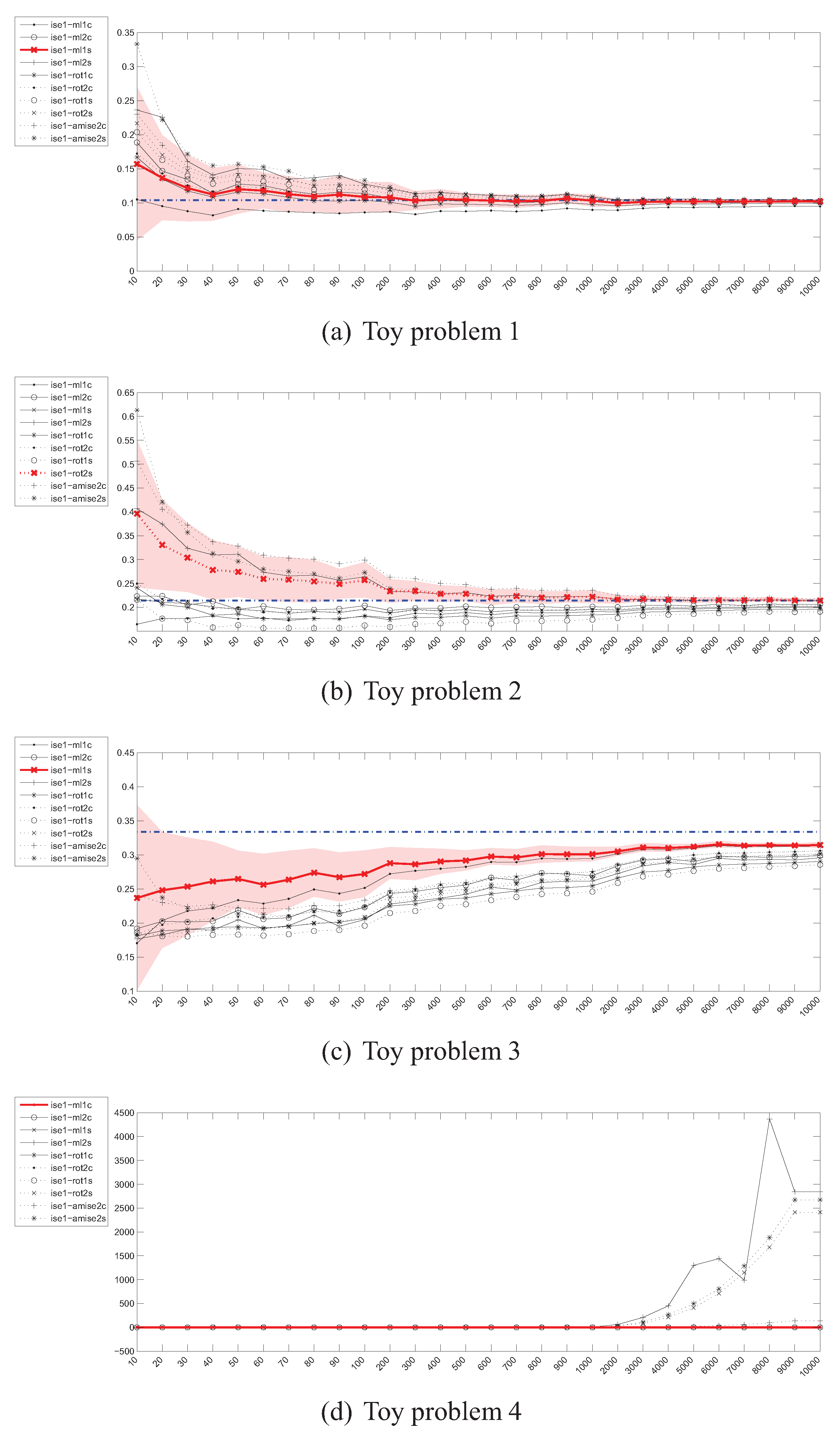
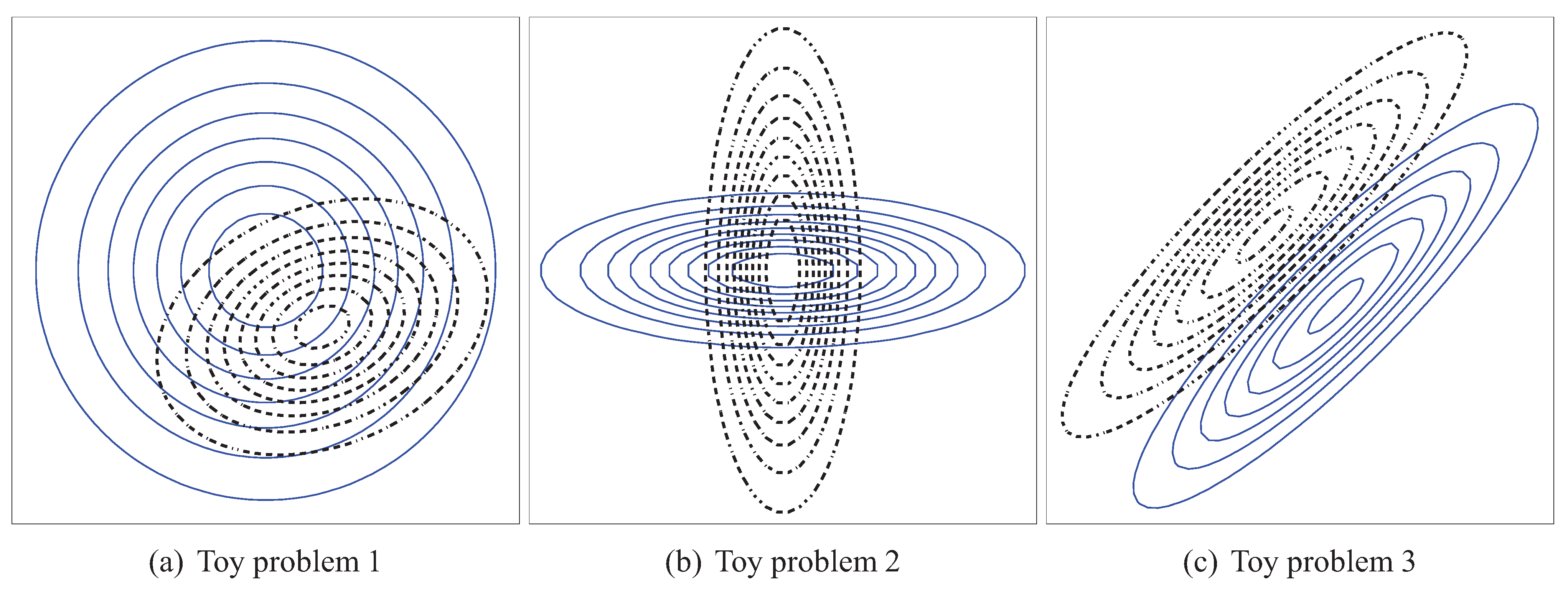
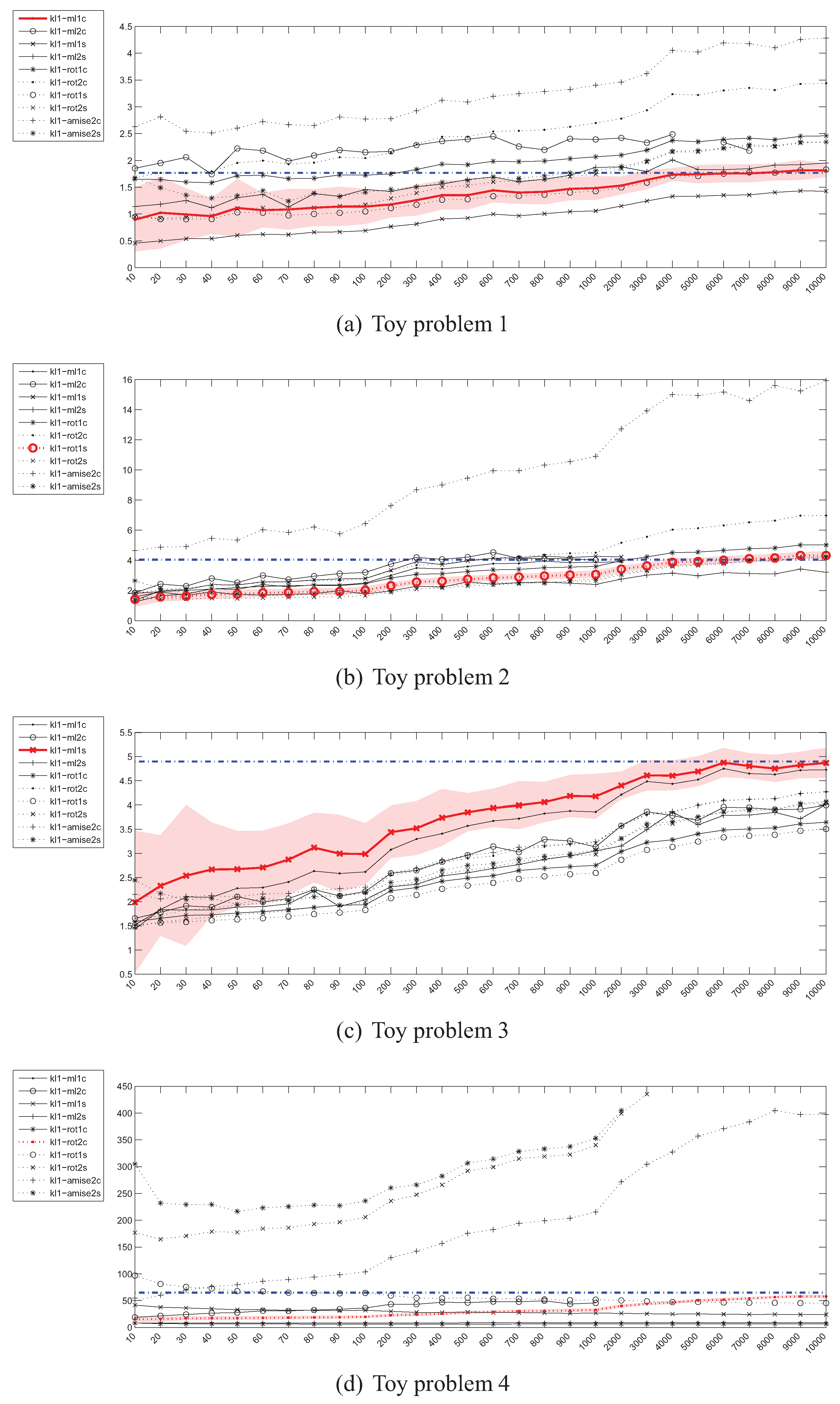
• Problem 1, which is the same as the one in [18]:

  $$\begin{array}{cc}{\mu }_p=\left[\begin{array}{c}0\\ 0\end{array}\right],\hfill & {\Sigma }_p=\left[\begin{array}{cc}1& 0\\ 0& 1\end{array}\right]\hfill \\ \\ {\mu }_q=\left[\begin{array}{c}0.5\\ -0.5\end{array}\right],\hfill & {\Sigma }_q=\left[\begin{array}{cc}0.5& 0.1\\ 0.1& 0.3\end{array}\right]\hfill \end{array}$$

  (24)
• Problem 2, where the means of both distributions are equal, but the covariance matrices are not:

  $$\begin{array}{cc}{\mu }_p=\left[\begin{array}{c}0\\ 0\end{array}\right],\hfill & {\Sigma }_p=\left[\begin{array}{cc}1& 0\\ 0& 0.1\end{array}\right]\hfill \\ \\ {\mu }_q=\left[\begin{array}{c}0\\ 0\end{array}\right],\hfill & {\Sigma }_q=\left[\begin{array}{cc}0.1& 0\\ 0& 1\end{array}\right]\hfill \end{array}$$

  (25)
• Problem 3, where the covariance matrices of both distributions are equal, but the means are not:

  $$\begin{array}{cc}{\mu }_p=\left[\begin{array}{c}0.35\\ -0.35\end{array}\right],\hfill & {\Sigma }_p=\left[\begin{array}{cc}1& 0.9\\ 0.9& 1\end{array}\right]\hfill \\ \\ {\mu }_q=\left[\begin{array}{c}-0.35\\ 0.35\end{array}\right],\hfill & {\Sigma }_q=\left[\begin{array}{cc}1& 0.9\\ 0.9& 1\end{array}\right]\hfill \end{array}$$

  (26)
• Problem 4, where the Gaussians are 20-dimensional, ${\mu }_p={\left[\begin{array}{cccc}0& 0& \dots & 0\end{array}\right]}^T$, ${\Sigma }_p=\mathit{I}$ and ${\mu }_q$, ${\Sigma }_q$ have been generated randomly from the $[-1,+1]$ and $[0,+2]$ intervals respectively.

For each experiment, 100 random samples of an exponentially increasing size were drawn from both $p\left(x\right)$ and $q\left(x\right)$. The divergence estimate was then calculated as the mean value of estimates for each of these 100 samples.

Denoting by d the dimensionality of the distributions, the Kullback-Leibler divergence between two Gaussian distributions $p_G\left(x\right)$ and $q_G\left(x\right)$ can be calculated using [43]:

$$\begin{array}{cc}\hfill D_{KL}(p_G,q_G)& =\frac{1}{2}\left(log\left(\frac{det{\Sigma }_q}{det{\Sigma }_p}\right)+Tr\left({\Sigma }_q^{-1}{\Sigma }_p\right)+{\left({\mu }_q-{\mu }_p\right)}^T{\Sigma }_q^{-1}\left({\mu }_q-{\mu }_p\right)-d\right)\hfill \end{array}$$

(27)

Calculation of the Jeffrey’s divergence between two Gaussian PDFs is straightforward, as $D_J(p_G,q_G)=D_{KL}(p_G,q_G)+D_{KL}(q_G,p_G)$.

In order to calculate $D_{CS}$ and $ISE$ exactly for the special case of two Gaussian distributions, the following Gaussian multiplication formula is used:

$$G(x-{\mu }_p,{\Sigma }_p)G(x-{\mu }_q,{\Sigma }_q)=G({\mu }_p-{\mu }_q,{\Sigma }_p+{\Sigma }_q)G(x-{\mu }_{pq},{\Sigma }_{pq})$$

(28)

where the exact expression for ${\mu }_{pq}$ and ${\Sigma }_{pq}$ in this case are irrelevant, as shown below. Using (28), the following holds:

$$\begin{array}{cc}\hfill \int p_G^2\left(x\right)dx& =\int G({\mu }_p-{\mu }_p,{\Sigma }_p+{\Sigma }_p)G(x-{\mu }_{pp},{\Sigma }_{pp})dx=G(0,2{\Sigma }_p)\hfill \end{array}$$

(29)

$$\begin{array}{cc}\hfill \int q_G^2\left(x\right)dx& =\int G({\mu }_q-{\mu }_q,{\Sigma }_q+{\Sigma }_q)G(x-{\mu }_{qq},{\Sigma }_{qq})dx=G(0,2{\Sigma }_q)\hfill \end{array}$$

(30)

$$\begin{array}{cc}\hfill \int p_G\left(x\right)q_G\left(x\right)dx& =\int G({\mu }_p-{\mu }_q,{\Sigma }_p+{\Sigma }_q)G(x-{\mu }_{pq},{\Sigma }_{pq})dx=G({\mu }_p-{\mu }_q,{\Sigma }_p+{\Sigma }_q)\hfill \end{array}$$

(31)

From the above and (17) and (20) the closed-form solutions for $D_{CS}$ and $ISE$ are:

$$\begin{array}{cc}& D_{CS}(p_G,q_G)=-log\frac{G({\mu }_p-{\mu }_q,{\Sigma }_p+{\Sigma }_q)}{\sqrt{G(0,2{\Sigma }_p)G(0,2{\Sigma }_q)}}\hfill \end{array}$$

(32)

$$\begin{array}{cc}& ISE(p_G,q_G)=\int p_G^2\left(x\right)dx+\int q_G^2\left(x\right)dx-2\int p_G\left(x\right)q_G\left(x\right)dx\hfill \\ & =G(0,2{\Sigma }_p)+G(0,2{\Sigma }_q)-2G({\mu }_p-{\mu }_q,{\Sigma }_p+{\Sigma }_q)\hfill \end{array}$$

(33)

Unfortunately, there is no closed-form formula to calculate the Jensen-Shannon divergence, and an estimate based on (6) calculated for $N_p=N_q=100000$ had to be used:

$$D_{JS}(p_G,q_G)=\frac{1}{2}{D}_{KL}(p_G,\frac{1}{2}(p_G+q_G))+\frac{1}{2}{D}_{KL}(q_G,\frac{1}{2}(p_G+q_G))$$

(34)

where:

$$\begin{array}{cc}\hfill D_{KL}(p_G,\frac{1}{2}(p_G+q_G))& \approx \frac{1}{N_p}\sum _{i=1}^{N_p}log\frac{p_G\left(x_{pi}\right)}{\frac{1}{2}(p_G\left(x_{pi}\right)+q_G\left(x_{pi}\right))}\hfill \end{array}$$

(35)

$$\begin{array}{cc}\hfill D_{KL}(q_G,\frac{1}{2}(p_G+q_G))& \approx \frac{1}{N_q}\sum _{i=1}^{N_q}log\frac{q_G\left(x_{pi}\right)}{\frac{1}{2}(p_G\left(x_{qi}\right)+q_G\left(x_{qi}\right))}\hfill \end{array}$$

(36)

Note, that in both equations above the terms under the logarithms are not dependent on any PDF estimator-specific parameters, as the PDFs are given in analytical forms, so the sample mean is the only estimation required.

Figure 2, Figure 3, Figure 4, Figure 5, Figure 6, Figure 7, Figure 8, Figure 9 and Figure 10 present the results of the experiments for the 4 toy problems. The “best” estimate in each plot has been marked with bold red line. Additionally the confidence intervals (mean ± one standard deviation) for the best method were also plotted. The best estimator has been chosen according to the criterion of fast convergence to the true value of the estimated measure and lack of divergence after reaching that target value. The below scoring function has been proposed and used to chose the best estimator:

$$S={\left(\sum _{i=1}^{\left|\mathcal{M}\right|}{m}_i{\left({\overline{y}}_i-t\right)}^2\right)}^{-1}$$

(37)

where $\mathcal{M}=\{10,20,\dots ,100,200,\dots ,1000,2000,\dots ,10000\}$, ${\overline{y}}_i$ is the mean value of the estimator for the sample size $m_i$ and t is the true value of the divergence measure. Note that this scoring function heavily penalizes any deviation from the true value for large sample sizes, which in effect assigns low scores to estimators which have not converged or started to diverge.

In the figures below the following code has been used for denoting the divergence estimators:

$$\begin{array}{ccc}& XX-YYZZ& \text{for}\text{Parzen}\text{window}\text{density}\text{estimates}\hfill \\ & XX-k& \text{for}\text{kNN}\text{density}\text{estimates}\hfill \end{array}$$

where k is the number of nearest neighbours and the remaining symbols have been given in

Table 1. Divergence measure estimators.

XX	Description
kl1	Kullback-Leibler divergence estimator based on Parzen window density
kl2	Kullback-Leibler divergence estimator based on kNN density
j1	Jeffrey’s divergence estimator based on Parzen window density
j2	Jeffrey’s divergence estimator based on kNN density
js1	Jensen-Shannon divergence estimator based on Parzen window density
js2	Jensen-Shannon divergence estimator based on kNN density
cs	Cauchy-Schwarz divergence estimator
ise1	Integrated Squared Error estimator based on Parzen window density
ise2	Integrated Squared Error estimator based on kNN density
YY	Description
ml	Pseudo-likelihood cross-validation
rot	Rule of Thumb
amise	AMISE minimisation
ZZ	Description
1c	Identity covariance matrix multiplied by a scalar, common for both PDFs
2c	Diagonal covariance matrix, common for both distributions
1s	Identity covariance matrix multiplied by a scalar, separate for each PDF
2s	Diagonal covariance matrix, separate for each distribution

.

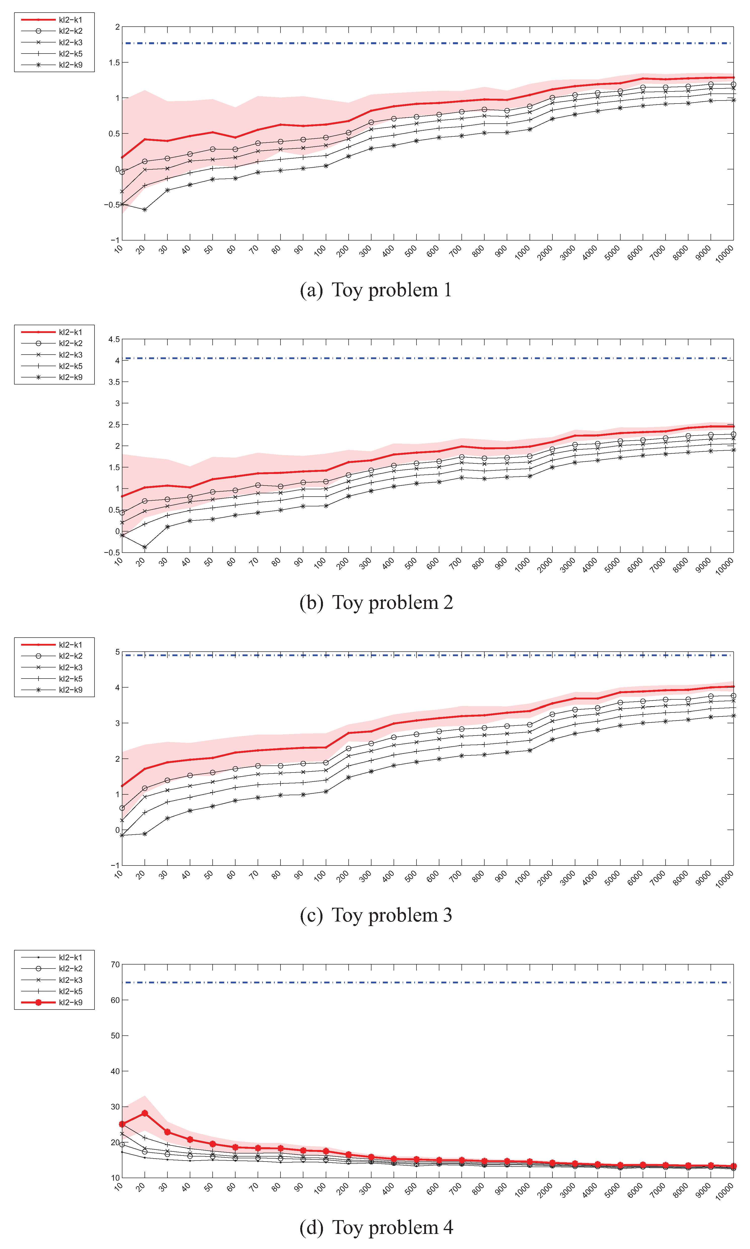
4.2. Estimation of the Kullback-Leibler (KL) Divergence

Figure 2 shows the plots presenting the evolution of Kullback-Leibler divergence estimators based on the Parzen window method as the sample size increases for all 4 toy problems. The values on the horizontal axis denote the number of instances drawn from each distribution. As it can be seen, there is a considerable discrepancy between various estimators (i.e., estimators using various bandwidth selection methods). More specifically, while some of them seem to be converging to the true value, others diverge, which is especially well visible in the case of high-dimensional toy problem 4. Moreover, even the “best” estimators reach the true divergence values for sample sizes, for which, if encountered in practice, the representativeness of even a random subsample should not be a problem. In such cases the purposefulness of divergence guided sampling seems doubtful.

Figure 3 presents the experimental results for Kullback-Leibler divergence estimators based on the kNN density estimator. In this case, the convergence for the 2-dimensional problems, albeit slow, can still be observed regardless of the value of k and has also been proven in [18]. However, for the 20-dimensional problem 4, the estimators fail completely.

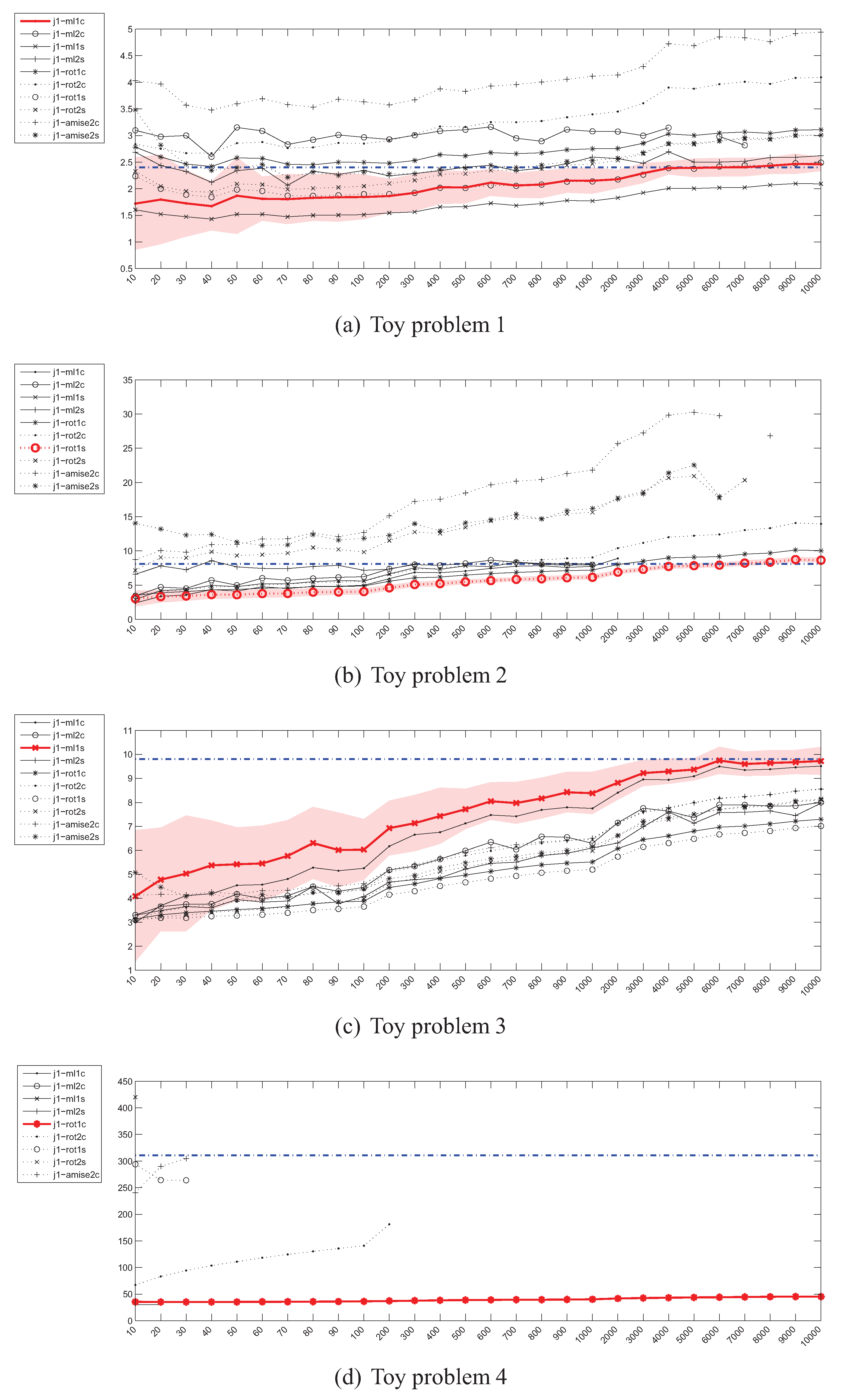
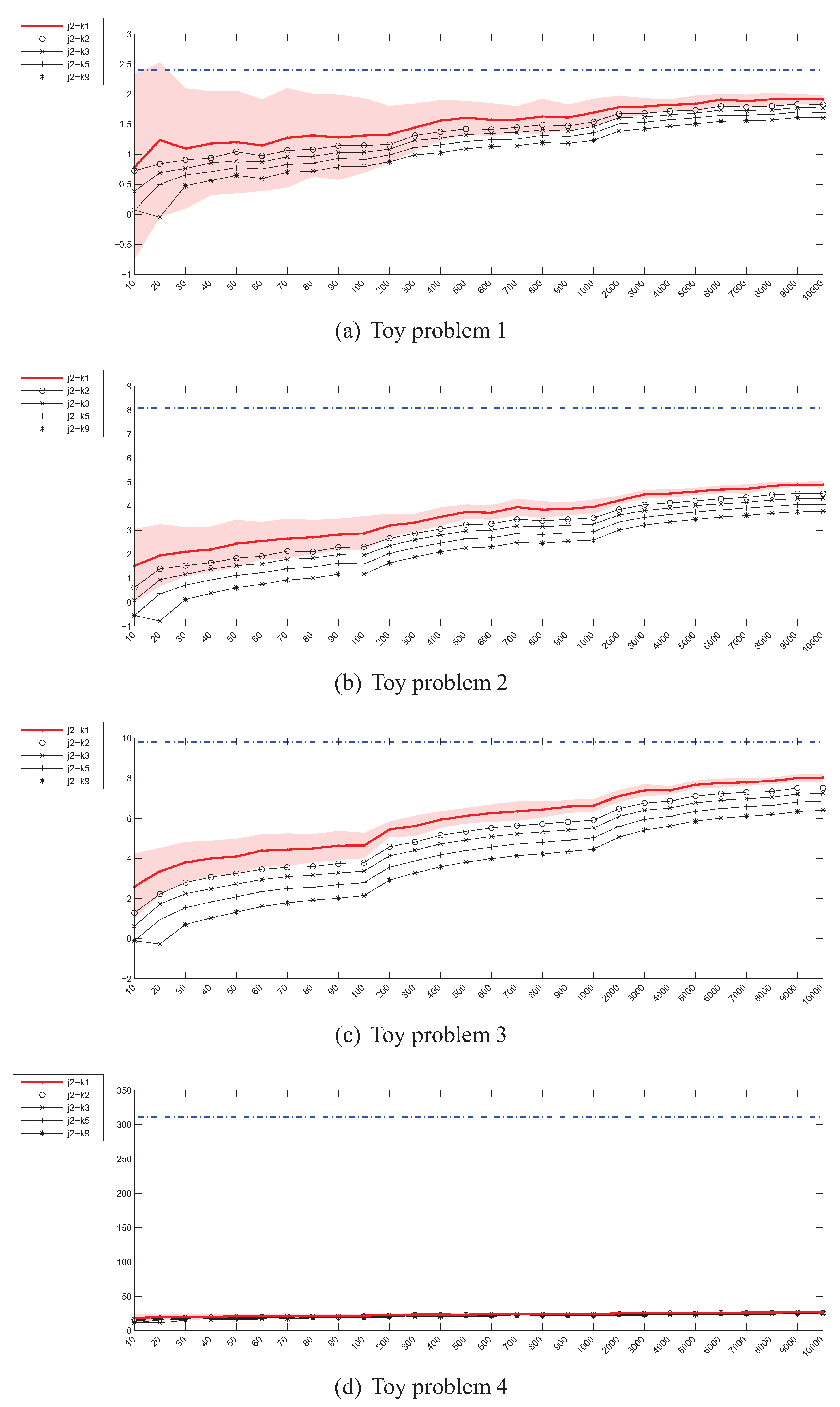
4.3. Estimation of the Jeffrey’s (J) Divergence

The behaviour of the Parzen window based estimators of the Jeffrey’s divergence has been depicted in Figure 4. For the 2-dimensional problems, the picture is very similar to the case of $D_{KL}$. However, in the high dimensional space most of the estimators cannot even be evaluated due to numerical problems, resulting from near-zero values of many Gaussian functions in calculation of ${\widehat{D}}_{KL}(q,p)$.

The Jeffrey’s divergence estimator based on kNN density depicted in Figure 5 also behaves in a way similar to ${\tilde{D}}_{KL}$. Although no numerical problems have been observed in the high-dimensional scenario, the estimators are off the true divergence value by a large margin.

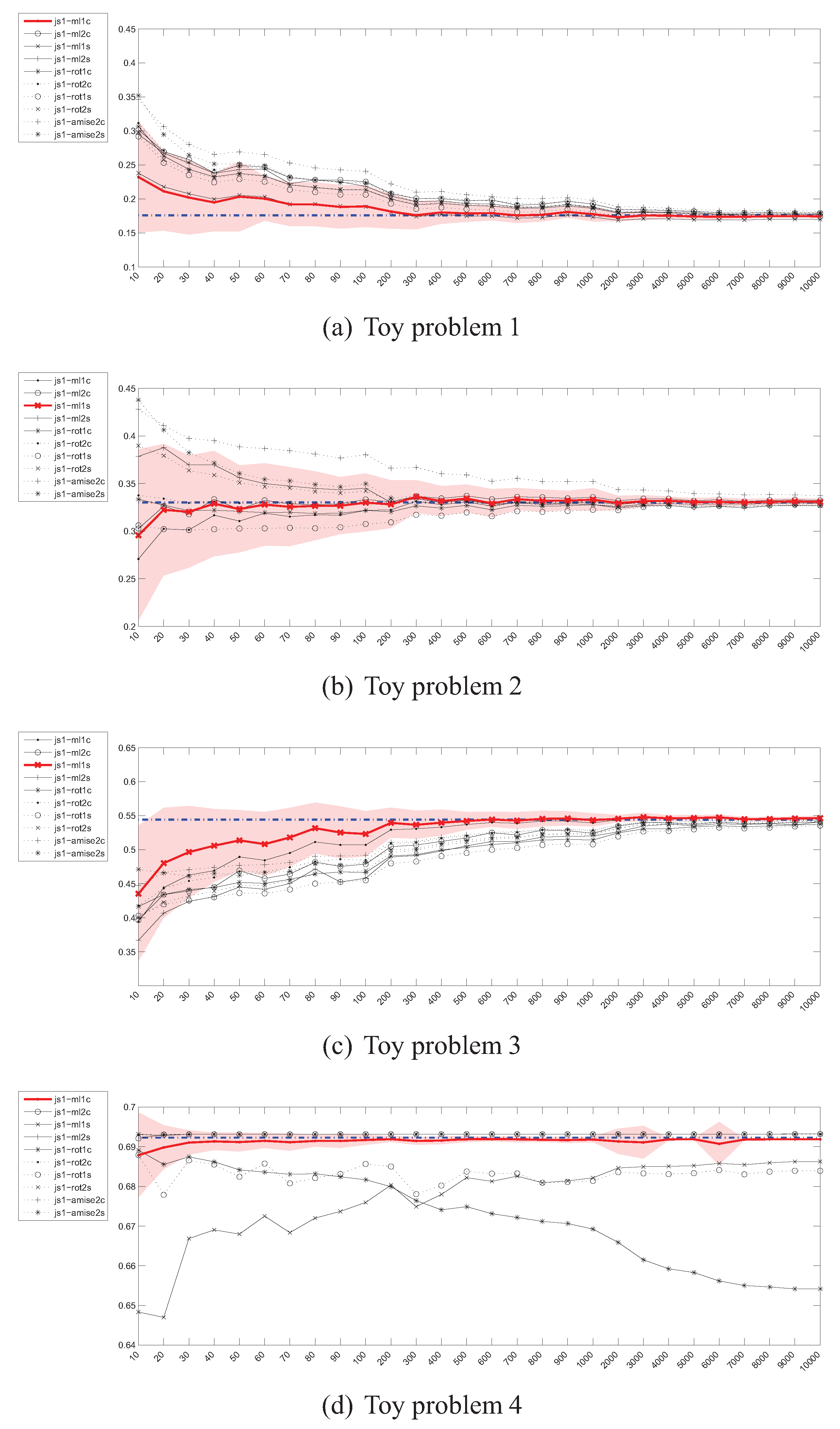
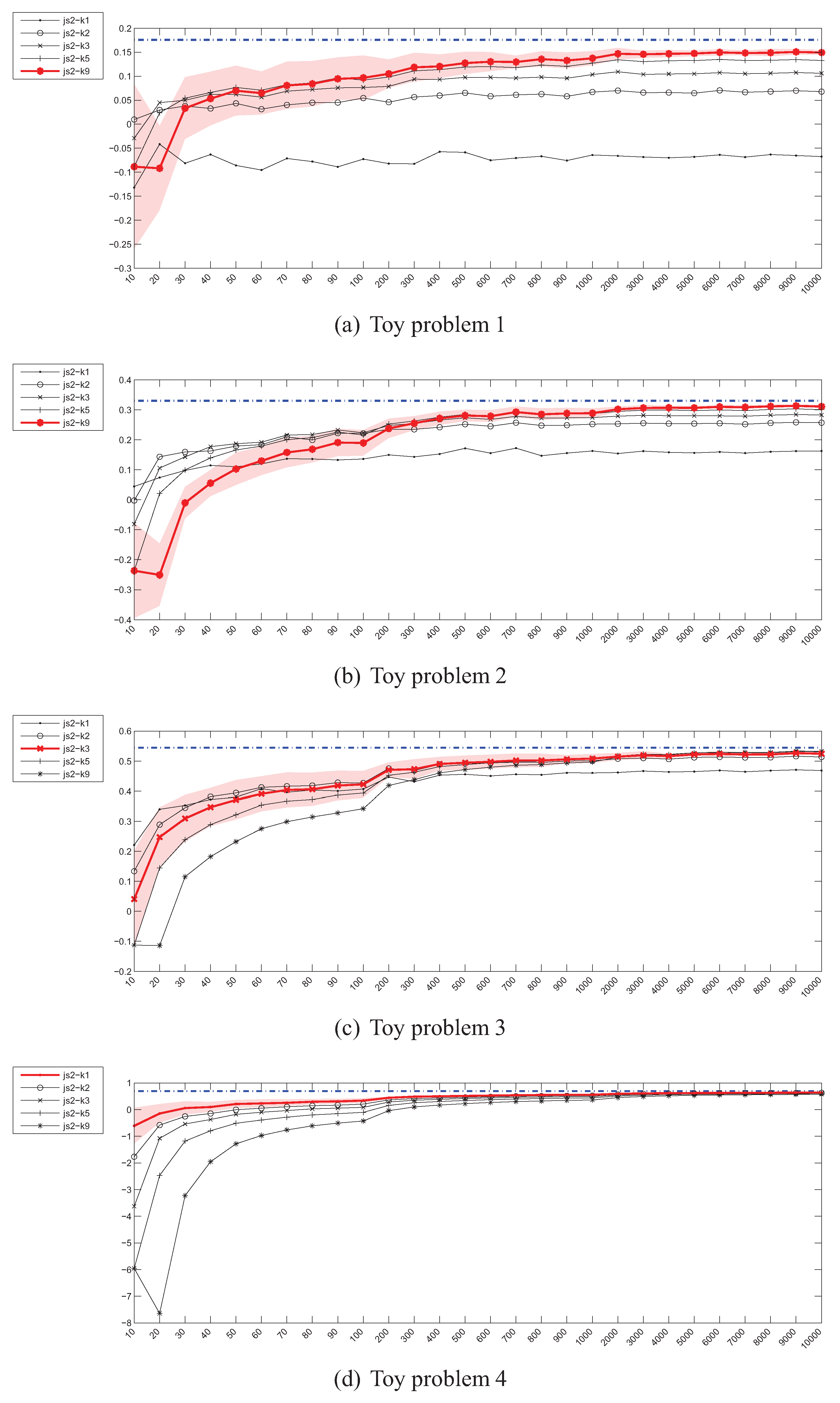
4.4. Estimation of the Jensen-Shannon’s (JS) divergence

The experimental results for the Jensen-Shannon’s divergence estimators given in Figure 6 and Figure 7 look much more promising. The convergence of the Parzen window based estimators is rapid when compared to ${\widehat{D}}_{KL}$ and ${\widehat{D}}_J$, as it takes place for sample sizes of 400–500. What is even more important is that, the estimators, regardless of the bandwidth selection method used, are usually in agreement when the shapes of the convergence curves are taken into account (the exception is the 20-dimensional problem). It should however be kept in mind that no closed-form formula for calculation of the true value exists, so effectively in this setting an estimate of the true value is approximated.

Although most of the kNN density based estimators also seem to be converging to the true value, the convergence is considerably slower than in the case of their Parzen window based counterparts. This can be seen by examining the units on the vertical axes in Figure 6 and Figure 7.

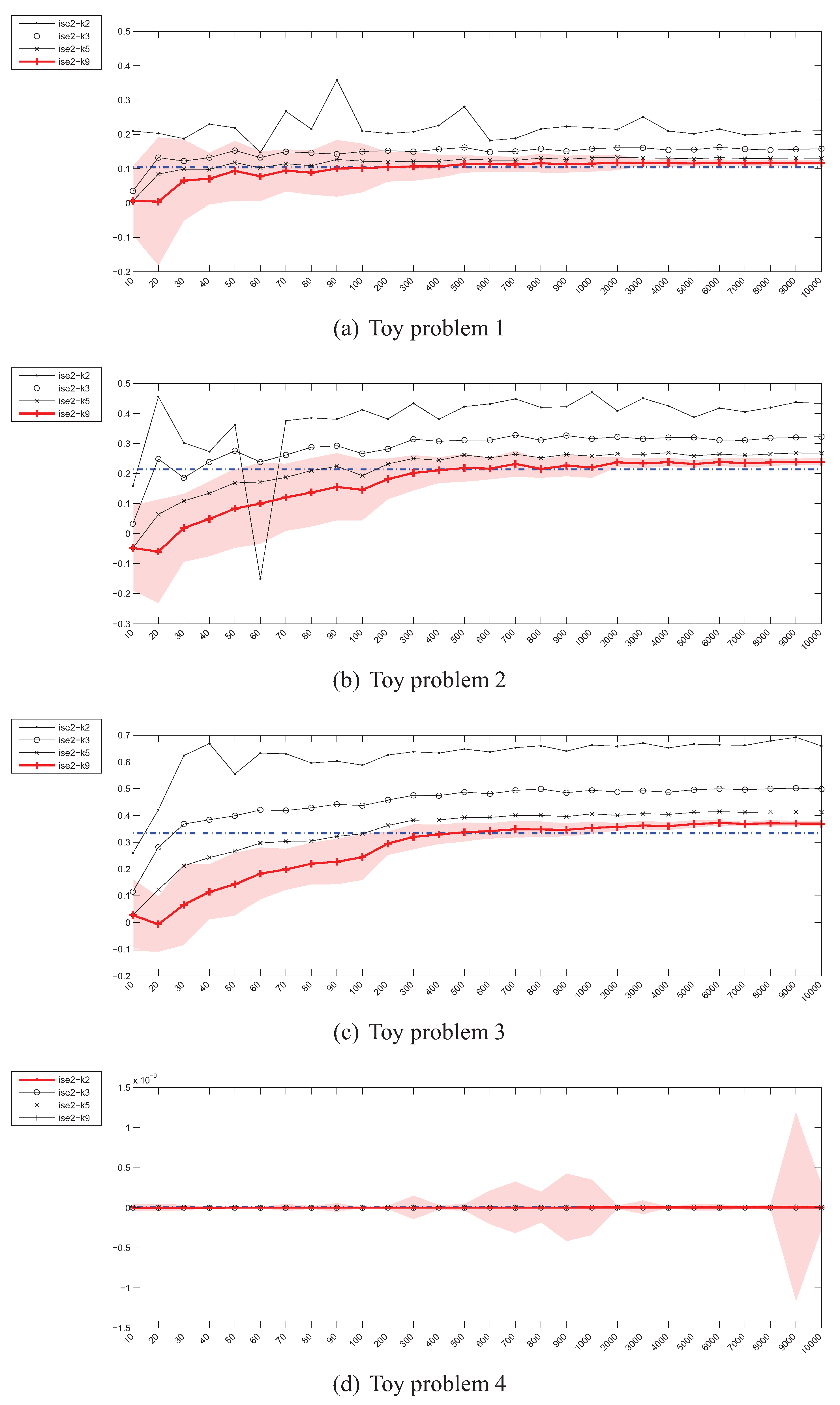
4.5. Estimation of the Integrated Squared Error (ISE)

The convergence curves for the Integrated Squared Error estimates have been depicted in Figure 8 and Figure 9. For the first two toy problems, the Parzen window based estimators behave in a desired way, relatively quickly approaching the true value of ISE. The situation looks a bit different in case of the toy problem 3, where for the examined sample sizes none of the estimators approaches the true value within 0.05. An interesting situation has however developed in the case of toy problem 4—throughout the whole range of sample sizes most estimators are very close to the true value, which at $1.0184e-011$ is itself very close to 0 and can pose numerical problems.

The situation for kNN density based estimators looks even more interesting. For small values of k (1 and 2) the estimator is unstable and its values vary greatly with the sample size. For this reason the $k=1$ case has not been included in the plots. The estimators also in general diverge and behave suspiciously in the 20-dimensional case.

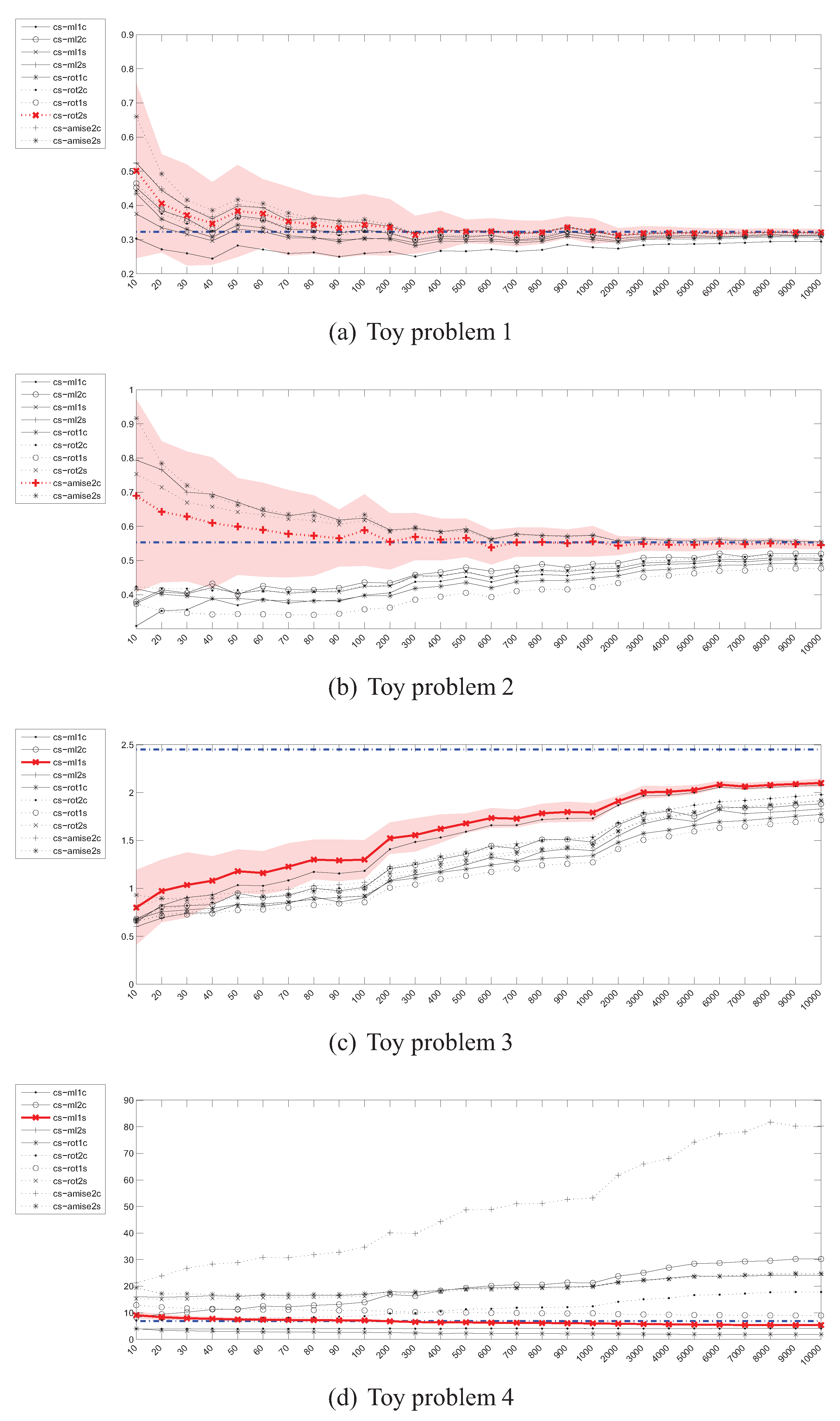
4.6. Estimation of the Cauchy-Schwarz (CS) divergence

The experimental results for the estimation of the Cauchy-Schwarz divergence can be seen in Figure 10. Although as mentioned in Section 3.4, as opposed to other divergence measures, in this case the only approximation is the Parzen windowing itself (no need to use (7)), the behaviour of ${\widehat{D}}_{CS}$ is not as good as one would expect. More specifically, the estimator did not reach the true value even for a sample of 10000 instances in the case of toy problem 3 and has diverged in the 20-dimensional scenario.

4.7. Summary

The picture emerging from the experimental results does not look very optimistic. Many estimates of various divergence measures either diverge or converge too slowly, questioning their usefulness for the purpose pursued in this study. From all the estimators examined, the Parzen window based Jensen-Shannon’s divergence estimator looks most promising, as it converges relatively quickly although it also demonstrates a considerable variance before converging—even for a sample of 10 instances the true value is within one standard deviation from the mean value of the estimate.

A common problem is also the behaviour of most estimators in a high dimensional space. In this case only ${\widehat{D}}_{JS}$ and ${\tilde{D}}_{JS}$ seem to be acting reasonably (once again, note the units on the vertical axes in Figure 6d and Figure 7d but in general Parzen windowing with kernels with exponential fall-off is known to be problematic, as the density in large areas of the high-dimensional space is necessarily close to 0.

It is also important to have in mind that all the toy problems examined are relatively simple, as they consist of symmetric, unimodal distributions, which unfortunately are rarely encountered in practice. As a result we can already expect the divergence estimation for real-world datasets to be even more difficult.

On the basis of the above experiments it is also very difficult to state what should be a minimal sample size for the divergence estimate to be accurate. There are at least two factors one needs to have in mind: the dimensionality of the PDF and its shape. The higher the dimensionality the more samples are needed to cover the input space and reflect the true underlying distribution. The same applies to the shape of the PDF—a spherical Gaussian can be described with a much lower number of samples than, e.g., some complex distribution with a lot of peaks and valleys. Moreover, the minimum sample size depends not only on the problem but also on the divergence estimator used. As can be seen in the above experiments even for a single problem and a fixed sample size, one estimator could have already converged, while another requires a sample twice as big for convergence.

5. PDF Divergence Guided Sampling for Error Estimation

In this section an empirical study of correlation between various PDF divergence estimators and bias of a generalisation error estimate is investigated using a number of benchmark datasets. Although as shown in Section 4, the PDF divergence measures are rather difficult to estimate, they can still be useful in the context of ranking PDFs according to their similarity to a given reference distribution. The goal of these experiments is thus to assess the possibility of estimating the generalisation error in a single run, i.e., without retraining the used model, by taking advantage of PDF divergence estimators within the sampling process. This would allow to further reduce the computational cost of error estimation when compared to both CV and DPS.

5.1. Experiment Setup

The experiments have been performed using 26 publicly available datasets (

Table 2. Benchmark datasets summary.

Acronym	Name	Source	#obj	#attr	#class
azi	Azizah dataset	PRTools	291	8	20
bio	Biomedical diagnosis	PRTools	194	5	2
can	Breast cancer Wisconsin	UCI	569	30	2
cba	Chromosome bands	PRTools	1000*	30	24
chr	Chromosome	PRTools	1143	8	24
clo	Clouds	ELENA	1000*	2	2
cnc	Concentric	ELENA	1000*	2	2
cnt	Cone-torus	[44]	800	3	2
dia	Pima Indians diabetes	UCI	768	8	2
ga2	Gaussians 2d	ELENA	1000*	2	2
ga4	Gaussians 4d	ELENA	1000*	4	2
ga8	Gaussians 8d	ELENA	1000*	8	2
gla	Glass identification data	UCI	214	10	6
ion	Ionosphere radar data	UCI	351	34	2
iri	Iris dataset	UCI	150	4	3
let	Letter images	UCI	1000*	16	26
liv	Liver disorder	UCI	345	6	2
pho	Phoneme speech	ELENA	1000*	5	2
seg	Image segmentation	UCI	1000*	19	7
shu	Shuttle	UCI	1000*	9	7
son	Sonar signal database	UCI	208	60	2
syn	Synth-mat	[45]	1250	2	2
tex	Texture	ELENA	1000*	40	11
thy	Thyroid gland data	UCI	215	5	3
veh	Vehicle silhouettes	UCI	846	18	4
win	Wine recognition data	UCI	178	13	3

* The number of instances actually used in the experiments, selected randomly with stratified sampling from the whole, much larger dataset in order to keep the experiments computationally tractable

) and 20 classifiers (

Table 3. Classifiers used in the experiments.

Acronym	Source	Description
fisherc	PRTools	Fisher’s Linear Classifier
ldc	PRTools	Linear Bayes Normal Classifier
loglc	PRTools	Logistic Linear Classifier
nmc	PRTools	Nearest Mean Classifier
nmsc	PRTools	Nearest Mean Scaled Classifier
quadrc	PRTools	Quadratic Discriminant Classifier
qdc	PRTools	Quadratic Bayes Normal Classifier
udc	PRTools	Uncorrelated Quadratic Bayes Normal Classifier
klldc	PRTools	Linear Classifier using Karhunen-Loeve expansion
pcldc	PRTools	Linear Classifier using Principal Component expansion
knnc	PRTools	k-Nearest Neighbor Classifier
parzenc	PRTools	Parzen Density Classifier
treec	PRTools	Decision Tree Classifier
naivebc	PRTools	Naive Bayes Classifier
perlc	PRTools	Linear Perceptron Classifier
rbnc	PRTools	RBF Neural Network Classifier
svc	PRTools	Support Vector Machine classifier (C-SVM)
nusvc	PRTools	Support Vector Machine classifier (ν-SVM)
gfc	[46]	Gravity Field Classifier
efc	[46]	Electrostatic Field Classifier

). For each dataset the below procedure was followed:

• 400 stratified splits of the dataset have been generated, leaving $87.5\%$ of instances for training and $12.5\%$ instances for testing, which corresponds with the 8-fold CV and DPS as used in [1,2],
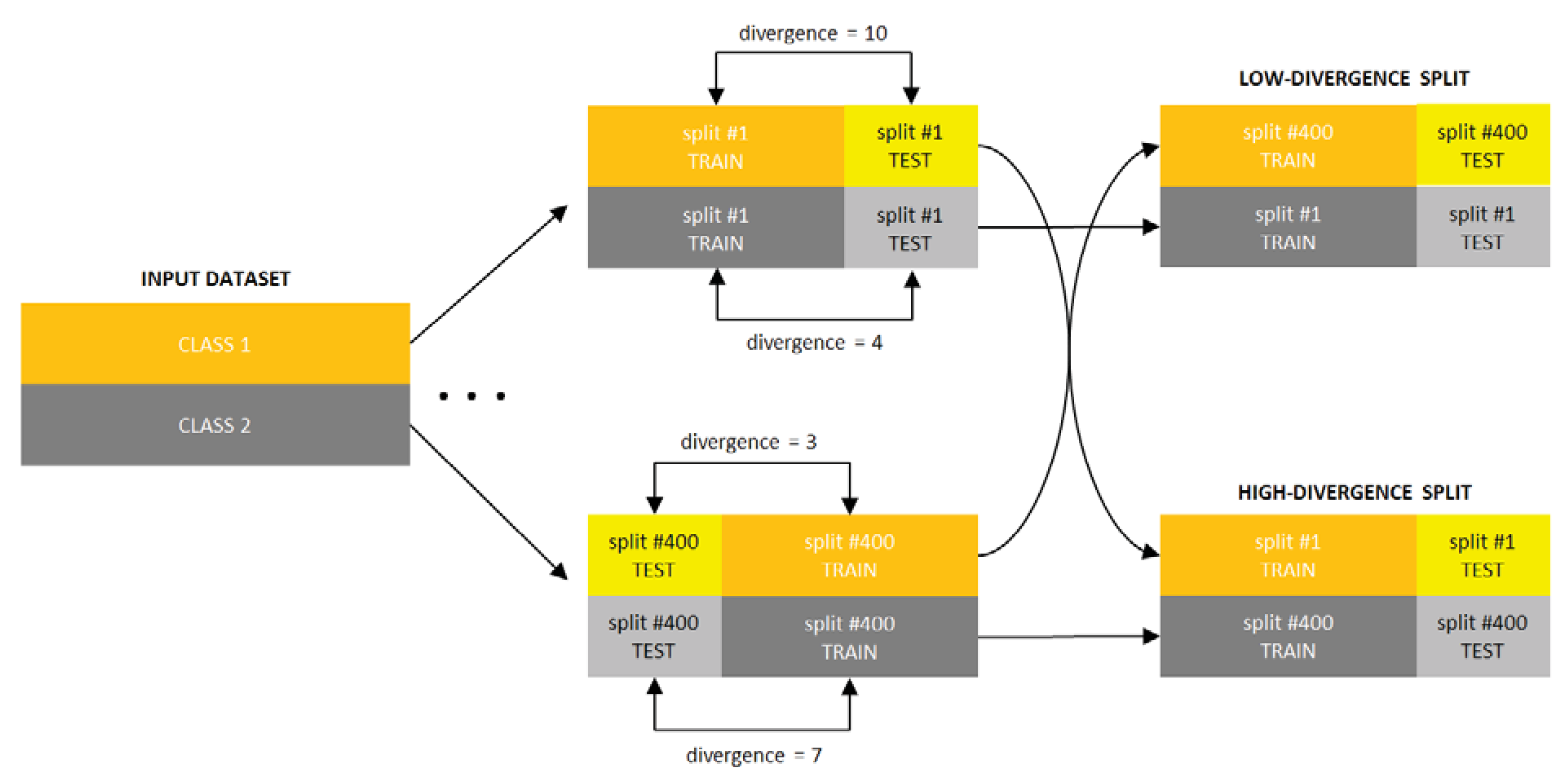
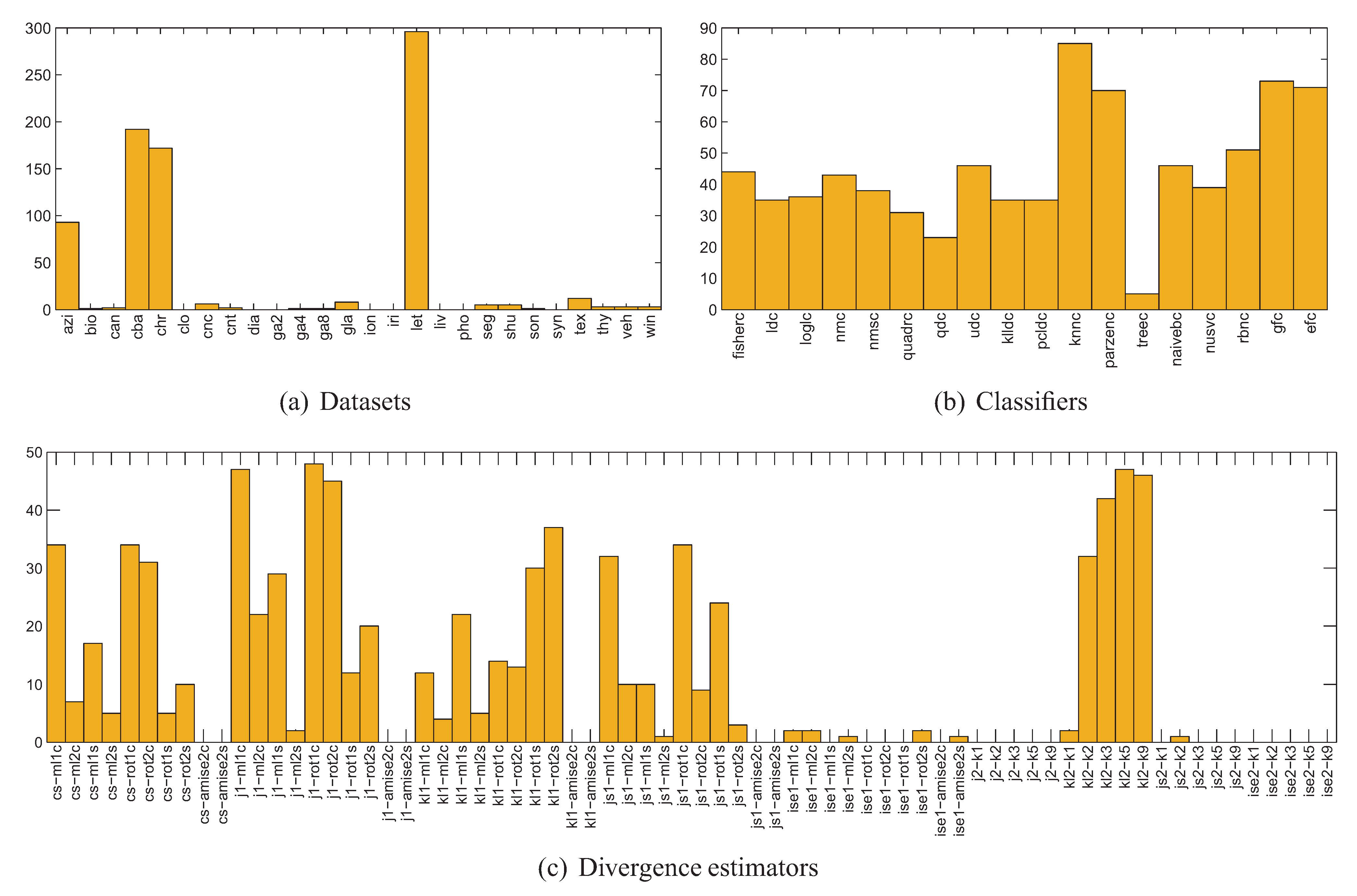
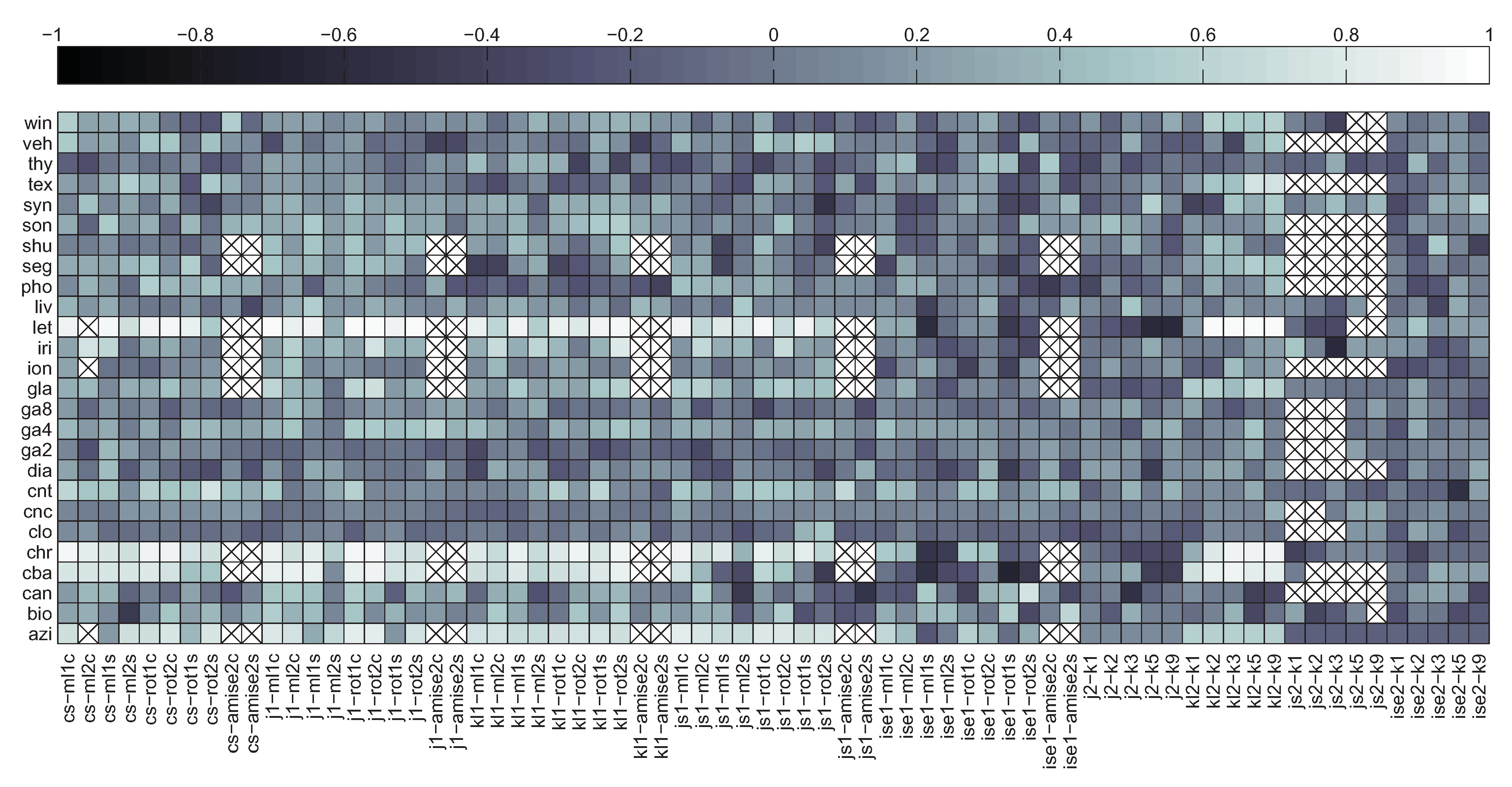
• for each of the 400 splits and each class of the dataset, 70 different estimators of divergence between the training and test parts were calculated, accounting for all possible combinations of techniques listed in Table 1, where in the case of kNN density based estimators $k=\{1,2,3,5,9\}$ were used; the rationale behind estimating the divergence for each class separately is that the dataset can only be representative of a classification problem if the same is true for its every class,
• for each divergence estimator the classes were sorted by the estimated value, forming 400 new splits per estimator (since for some splits some estimators produced negative values, these splits have been discarded),
• 11 splits were selected for each divergence estimator based on the estimated value averaged over all classes, including splits for the lowest and highest averaged estimate and 9 intermediate values,
• the classifiers were trained using the training part and tested using the test part for each split and each divergence estimator, producing error estimates sorted according to the divergence estimate.

The above procedure has been depicted in Figure 11.

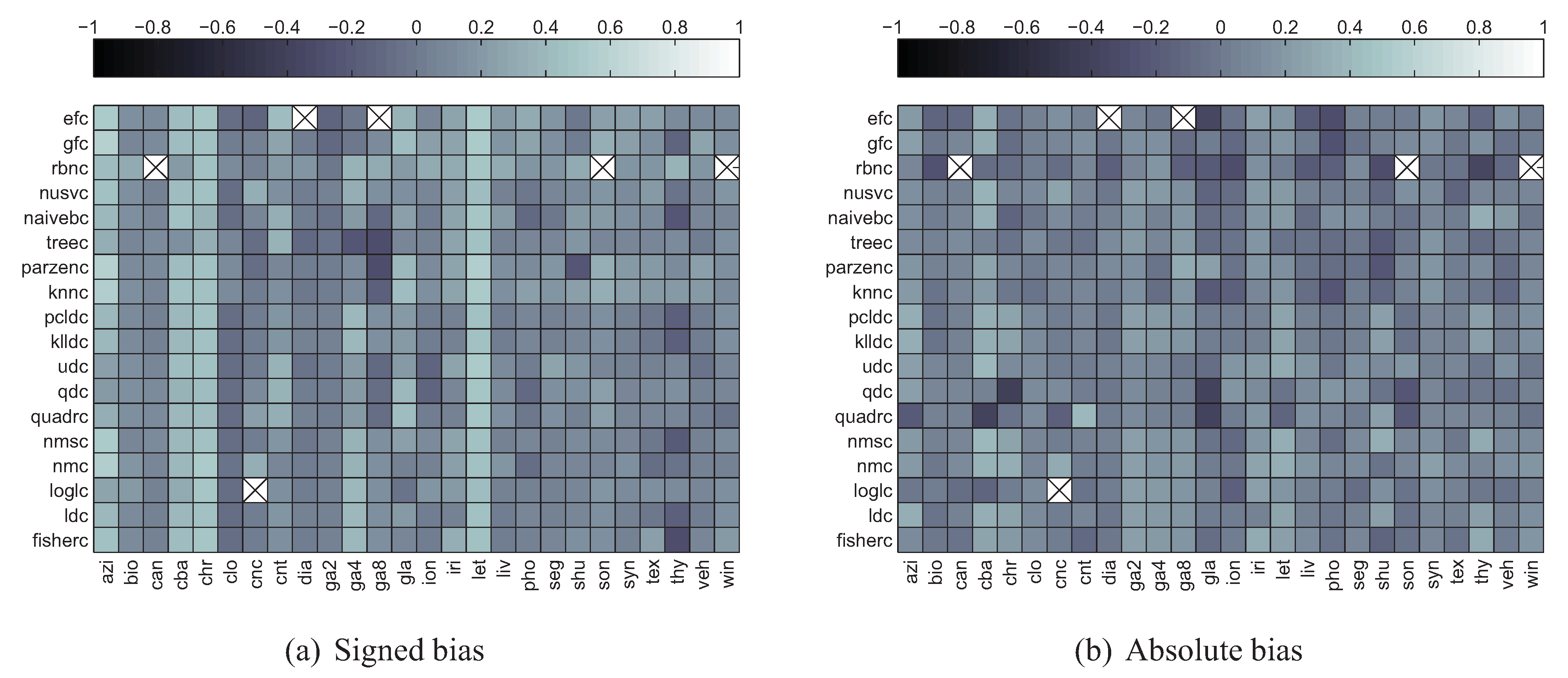
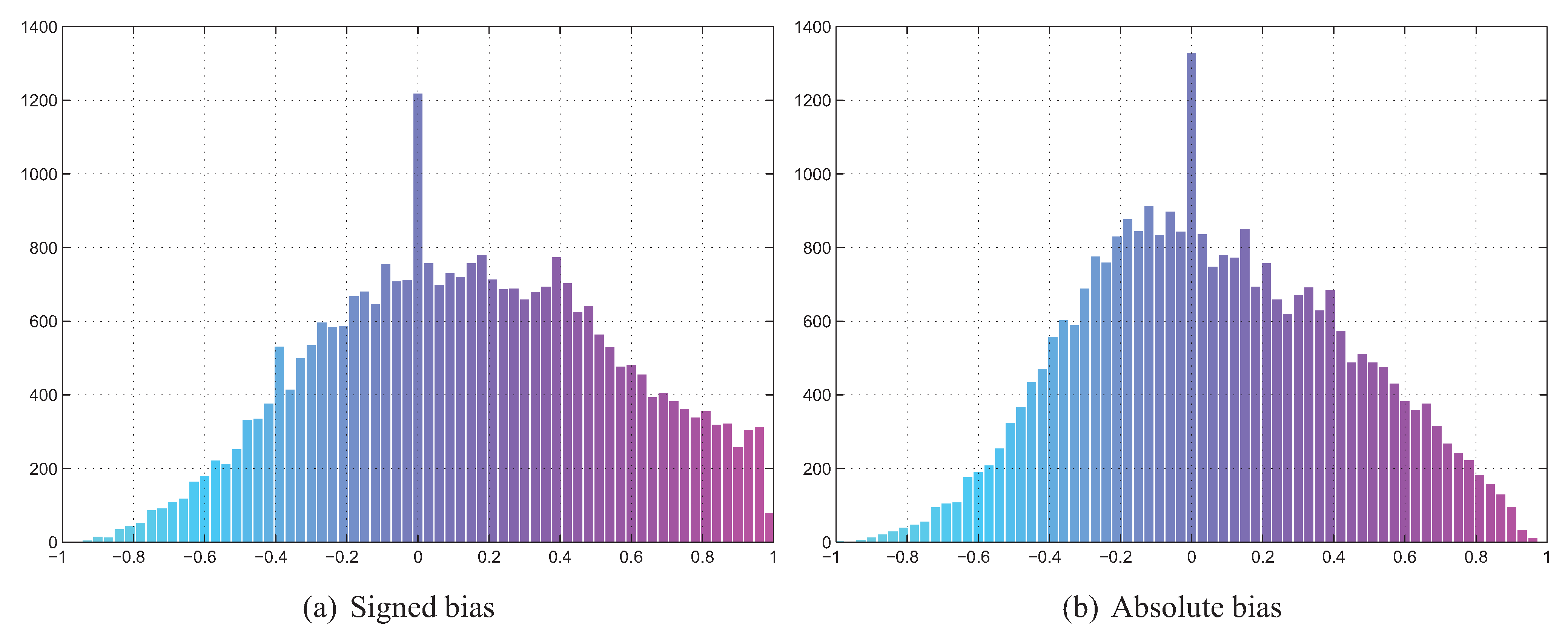
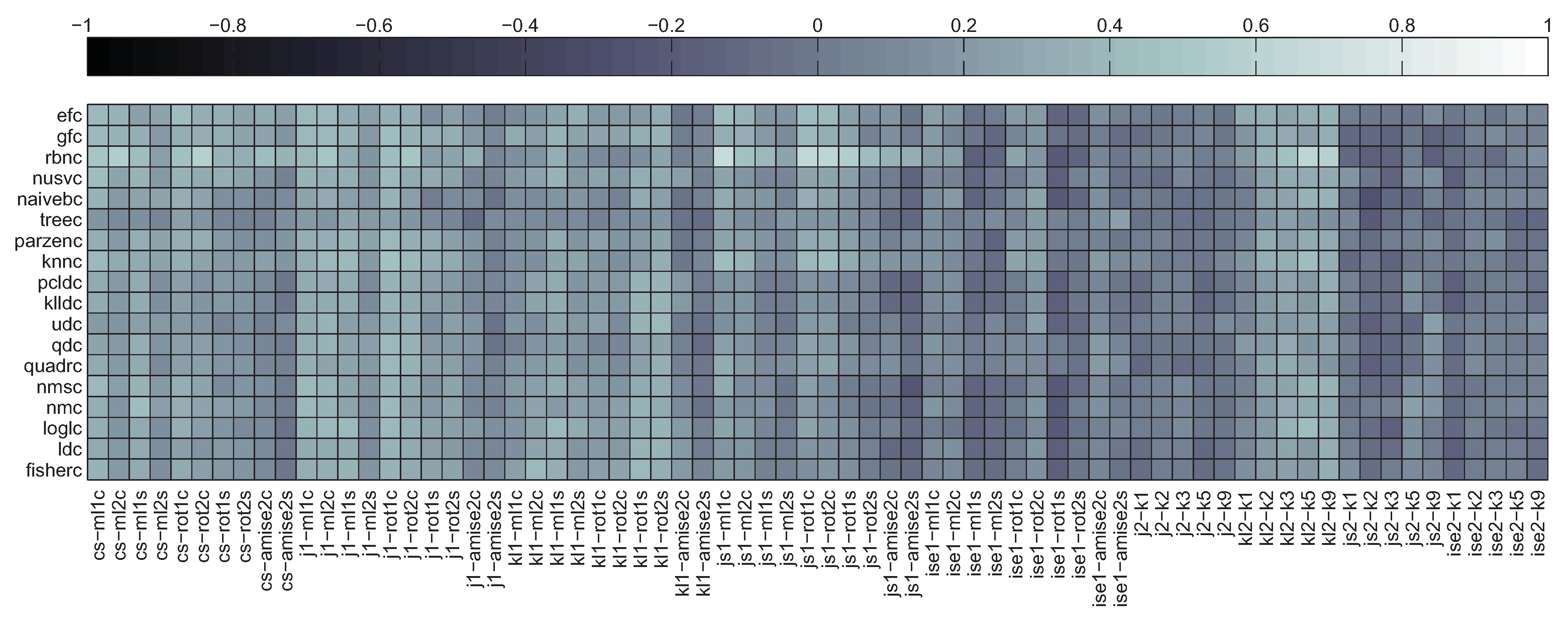
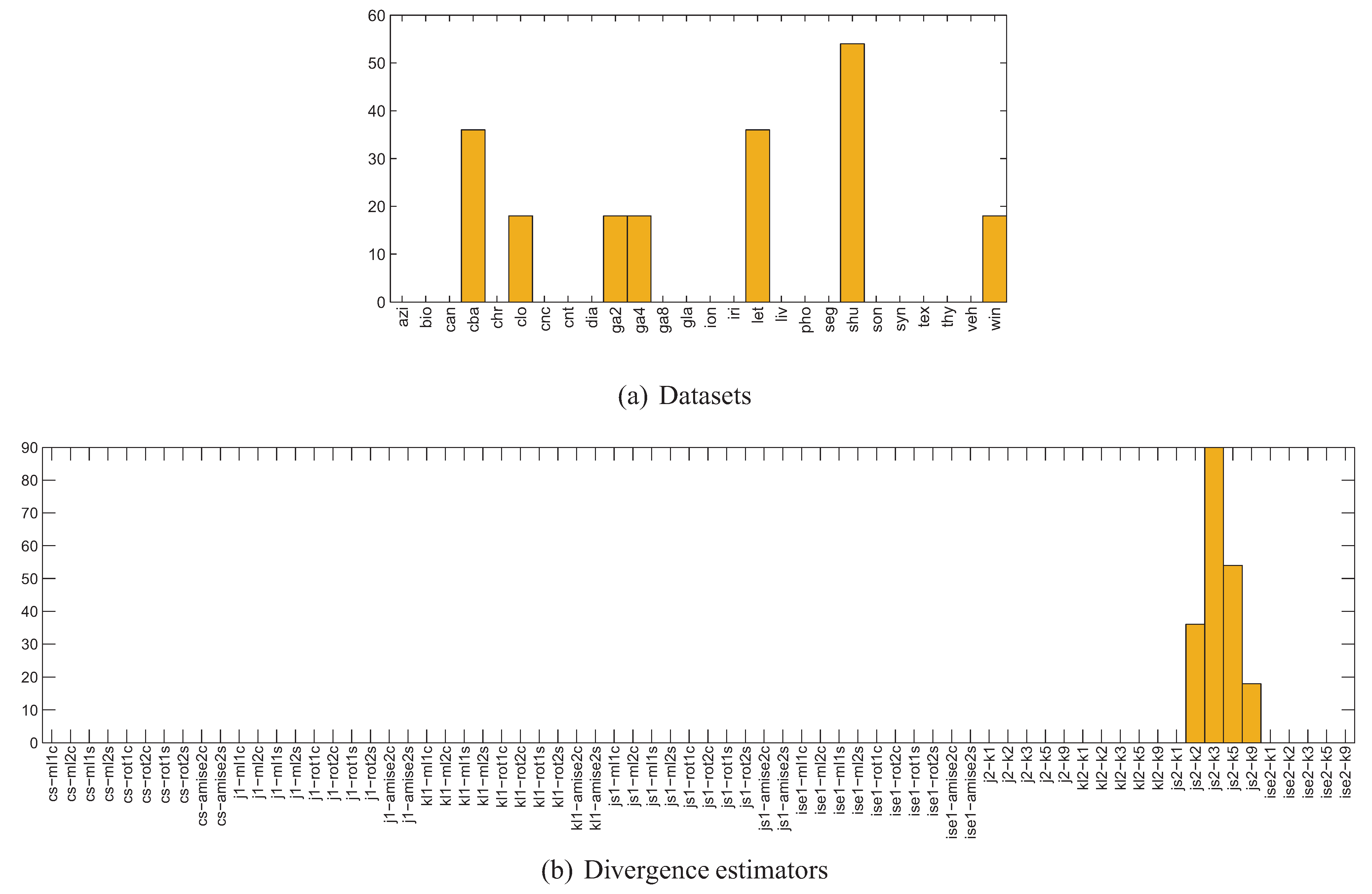
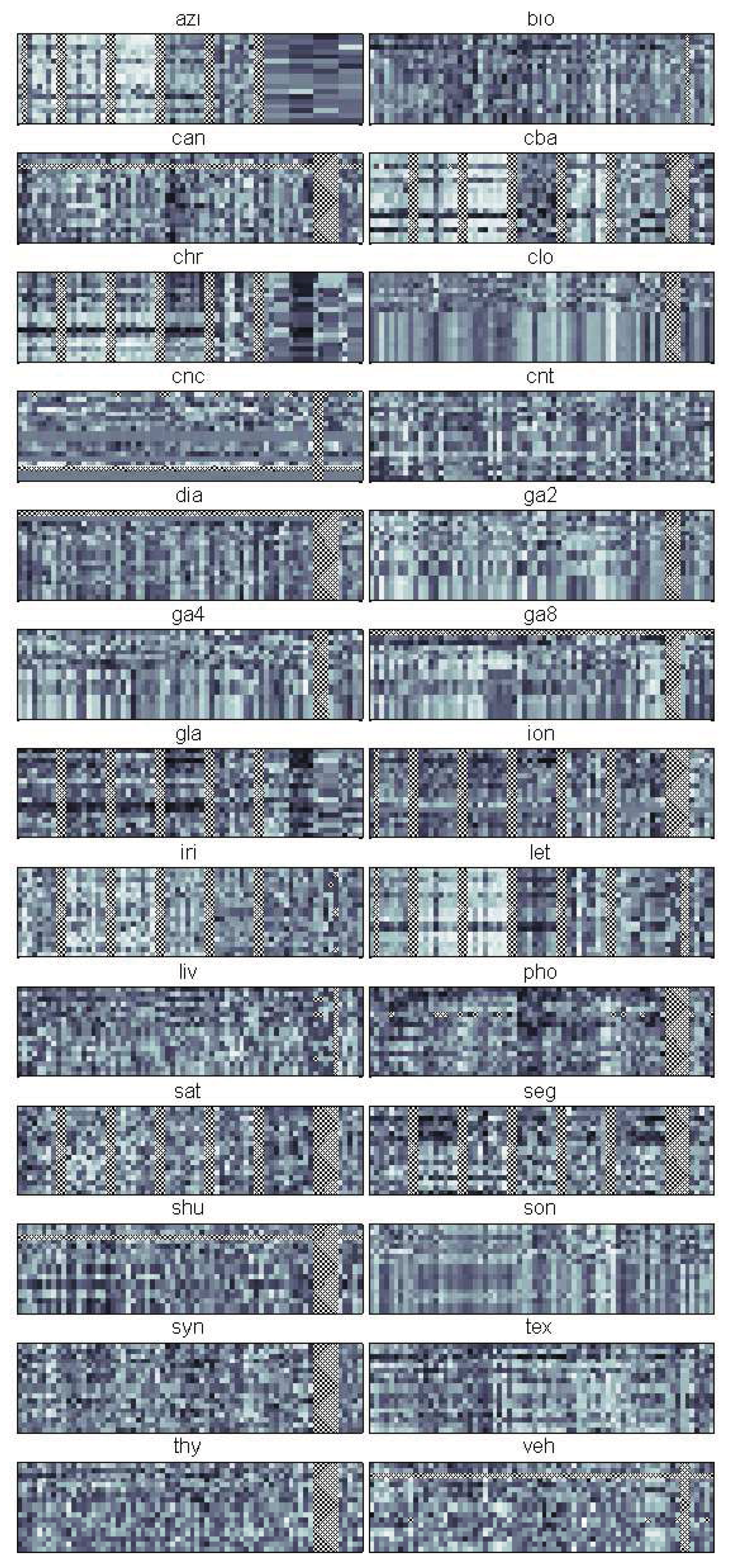
5.2. Correlation between Divergence Estimators and Bias

In the course of the experiments over 30,000 correlation coefficients have been calculated, accounting for all dataset/classifiers/divergence estimator triplets, with the exception of the cases in which calculation of correlation was not possible due to numerical problems during calculation of the divergence estimators (especially the ones based on AMISE bandwidth selection).

The maps of linear correlation coefficients between bias and divergence estimates, averaged over all divergence estimators used, have been depicted in Figure 12. The crossed-out cells denote the situation in which for all 11 splits both the values of divergence estimator and bias were constant, so it was impossible to assess correlation. As it can be seen, for the signed bias, moderate correlation can be observed only for a handful of datasets. However in some cases this applies to all (chr, let) or almost all (cba) classifiers. For other datasets the correlation is weak to none and sometimes even negative. Only occasional and rather weak correlation can be observed in the absolute bias scenario. This can be confirmed by looking at Figure 13 with histograms of correlation coefficients for all 30,000 dataset/classifier/divergence estimator triplets in both signed and absolute bias scenarios. Thus only the former scenario appears viable, as in the case of absolute bias the histogram is skewed towards $-1$ rather than 1.

One thing that requires explanation with respect to Figure 13 is the height of the bars centered at 0, for both signed and absolute bias. This is a result of cases in which the divergence estimator returned constant values for all 11 splits, although the bias varied. Figure 14 presents a more detailed breakdown of the 198 dataset/divergence estimator pairs for which this situation has occurred. As it can be seen, the kNN density based Jensen-Shannon’s divergence estimator ${\tilde{D}}_{JS}$ is to blame here, as it was unable to quantify the divergence in the case of 7 out of 26 datasets. When multiplied by the number of classifiers used, this gives over 3500 dataset/classifier/divergence estimator triplets with no correlation, accounting for more than a quarter of the 0-centered bars in the discussed figures. The problems caused by ${\tilde{D}}_{JS}$ come as a surprise, since this is the only estimator which was able to cope with the high-dimensional toy problem 4 discussed in Section 4.

Figure 15 depicts the signed bias correlation map averaged over all datasets, while in Figure 16 the map averaged over all classifiers has been given. The two figures confirm moderate correlation for some combinations of divergence measures and datasets. The crossed-out cells in Figure 16 reflect the numerical problems of the AMISE Parzen window bandwidth selection method and kNN density based Jensen-Shannon’s divergence estimator mentioned before.

Unfortunately, the averaged results presented so far tend to smooth out the fine details, which might provide more insight into the behaviour of individual methods. For that reason in Figure 17 the correlation maps have been given in a breakdown for each dataset. As it can be seen the highest correlation can be observed for the azi, cba, chr and let datasets, in all cases for roughly the same divergence estimators (all Parzen window based except for ise1 as well as the kNN based kl2). Unfortunately, for the remaining 22 datasets the situation does not look that well, although for each of them there are areas in the plot denoting medium to strong correlation.

Figure 18 presents the histograms of correlation coefficients for individual divergence estimators. As it can be seen, there is only a handful of estimates which demonstrate a certain degree of correlation with the bias, including some of the Cauchy-Schwarz and Kullback-Leibler divergence estimators and especially kl2-k3, kl2-k5 and kl2-k9. This seems to contradict the experimental results presented in Figure 3, where it can be seen, that the higher the number of neighbours, the slower the convergence of the kl2 estimators. In the case of kl2-k1 in Figure 18 however, the histogram is symmetric if not skewed to the left, while it changes its shape to more right-skewed as the number of nearest neighbours is increased.

In Figure 19 the histograms of datasets, classifiers and divergence estimators for the 806 high ($\ge 0.9$) signed bias correlation cases have been presented. The first observation is that the correlation is indeed strong only for 3 to 4 datasets and the divergence estimators already identified. The disappointing performance of the ise1, j2, js2 and ise2 estimators has also been confirmed. Also note, that although the histogram of classifiers does not present a uniform distribution, there are numerous high correlation cases for almost all classifiers, with knnc, gfc, efc taking the lead, and treec being the worst one.

The most surprising conclusion can however be drawn from examination of the four datasets, for which the high correlation has been observed. A closer look at Table 2 reveals that the one thing they have in common is a large number of classes, ranging from 20 to 24, while most of the remaining datasets have only 2 to 3 classes. Since in the experimental setting used, the divergences have been approximated for each class in separation, the estimates have been effectively calculated for very small sample sizes (the average class size for the let dataset is just 39 instances). From the experiments described in Section 4 it is however clear that for sample sizes of this order the estimates are necessarily far from converging, especially in the case of high-dimensional problems. However, in order to put things into perspective, one needs to realize that the 806 high correlation cases constitute just above 2.6% of the total number of over 30,000 cases. Thus effectively they form the tail of the distribution depicted in Figure 13 and most likely do not have any practical meaning.

For comparison with the results of [2], scatter plots of the 49 unique subsamples of the Cone-torus dataset for the lowest values of all divergence estimators used in the experiments have been depicted in Figure 20. The number in round brackets in the title of each plot denotes an identifier of the unique subset. The decision boundaries of a quadratic classifier (qdc) have also been superimposed on each plot. The classifier has been chosen due to its stability, so that any drastic changes in the shape of the decision boundaries can be attributed to considerable changes in the structure of the dataset used for training. In the majority of cases, the decision boundaries resemble the ones given in [2]. The same applies to the banana-shaped class, which is also clearly visible in most cases. This can be contrasted to Figure 21 containing the scatter plots of 49 unique subsets for the highest values of divergence estimators, where the decision boundaries take on a variety of shapes. As it can be seen though, the properties of the subsamples do depend on the values of the divergence estimators. For the Cone-torus dataset (cnt) there was however only a handful of high correlation cases. This behaviour is in fact very similar to that of DPS, where typically 7 out of 8 folds resembled the original dataset when examined visually. Thus although the examined divergence estimators were not able to produce a single fold allowing for generalisation error estimation, they could be used in a setting similar to the one presented in [2]. Note however, that correntropy used in the DPS approach is much easier to optimise, generating lower computational overhead than any other PDF divergence estimator examined in this paper.

5.3. Summary

The experiments performed in this section have shown that in general there is no correlation between various PDF divergence estimates and error estimation bias in classification problems. Since this correlation is a prerequisite for estimating the generalisation error in a single run, we conclude that it is not possible to estimate the generalisation in this way using tested divergence estimators.

6. Discussion

According to the experimental results presented in Section 4 it can be said, that in general the divergence between two PDFs is a quantity rather difficult to estimate. This holds regardless of the actual divergence measure one is trying to approximate although to a different extent. For example, in the case of the Kullback-Leibler divergence, the results are at least disappointing as the estimators often do not reach the true value even for 10,000 instances drawn from each distribution. Kullback-Leibler divergence is however one of the most widely used measures of this type.

In [23] the authors use the estimator of (10) to sample a reduced yet representative subset of the input dataset for the purpose of data condensation. The experimental setting was:

• Experiments based on Gaussian distributions, with (1) three 8-dimensional datasets consisting of two normally distributed classes with various configurations of means and covariances, (2) 100 instances drawn randomly per class, used for selection of representative subsample and parameter tuning (for each class separately), and (3) 100 instances drawn randomly per class for testing.
• Experiments based on non-Gaussian distributions, with (1) one dataset of unknown dimensionality having two classes, each distributed according to a mixture of two Gaussians (two-modal distributions), (2) 75 instances drawn randomly per each mode (i.e., 150 instances per class) for selection of representative subsample and parameter tuning (for each class separately), and (3) instances drawn randomly per each class for testing.
• Greedy optimisation of the Kullback-Leibler divergence estimator in both cases.

The authors report “excellent” results if three or more representatives from each class are selected in the case of the Gaussian datasets and six or more representatives in the non-Gaussian setting, although no numerical results are presented. According to the experimental results reported in Section 4 for sample size of 100 in most cases it is difficult to expect the ${\widehat{D}}_{KL}$ estimate to approximate the true divergence value well. However, by manipulating the kernel covariance matrix one is able to almost freely influence the value of the estimate. In the discussed paper, the authors have set the kernel covariance matrix to be equal to the sample covariance matrix, which led to excellent performance only on the Gaussian datasets. This is not surprising as in this case a single kernel function was able to approximate the class PDF well, if located correctly. If one also takes into account that a relatively stable quadratic classifier was used in the experiments, the results should be attributed to this specific experimental setting rather than to optimisation of the divergence. The authors admit that “the selection of kernel function and kernel covariance matrix is not clearly understood”, which suggests that it is the manual tuning of the covariance matrix which might be responsible for the “excellent” results in the non-Gaussian scenario.

Surprisingly in most of the literature the Kullback-Leibler or Jeffrey’s divergence is not estimated at all. Instead, it is either argued that optimisation of a given objective function is equivalent to optimisation of the divergence between an empirical measure and true yet unknown distribution (e.g., [47,48]) or closed-form solutions are used, restricting the PDFs to be Gaussian (e.g., [29,49]). Hence it appears that in practice $D_{KL}$ is mostly of theoretical interest, stemming from its connection to the information theory.

On the contrary, in [37] the authors use an estimator of the Jensen-Shannon divergence in a form similar to (14) but with a different kernel function. In their experimental setting the divergence estimator is calculated for two samples with sizes equal to 1024 and 10,240, which according to the results presented in Figure 6 is more than enough to obtain accurate estimates, even in a high-dimensional space.

Estimation of the divergence (and other measures for that matter) is hence always connected with a risk resulting from poor accuracy of the estimators, if the datasets do not contain thousands or tens of thousands of instances. This issue is however often neglected by other researchers. An example can be found in [41], where a Cauchy-Schwarz divergence-based clustering algorithm is derived. The authors report good performance for two synthetic, 2-dimensional datasets (419 instances, 2 clusters and 819 instances, 3 clusters) using the RoT method to determine the “optimal” Parzen window width and then heuristically annealing it around that value. These results more or less stay in agreement with the ones presented in Figure 10, although they might also be a result of manual tuning of the annealing process.

As for the second experimental part of this study, due to a wide range of datasets used, it can be stated that sampling by optimisation of any divergence measure estimator presented in Section 3 does not produce subsets, which lead to consistent observable estimation of the generalisation error. At this stage it is however difficult to state if the reason for this result is nonsuitability of the divergence measures used or poor accuracy of their estimators, especially in the light of the properties of the datasets for which high correlation has been identified.

7. Conclusions

In this paper, accuracy and empirical convergence of various PDF divergence estimation methods and their application to sampling for the purpose of generalisation error estimation have been evaluated. Five different divergence measures all having sound theoretical foundations have been examined, paired with two PDF estimators with various parameter settings, leading to 70 divergence estimators in total.

The most important outcome of this study is that the evaluated divergence measures can be estimated accurately only if large amounts of data are available. For some estimators and problems it is possible to obtain accurate estimates for sample sizes in the range of 400–600 instances, while in other cases even 10,000 instances is not sufficient. It is important to emphasize here that empirical convergence has been assessed using simple, synthetic problems with data sampled from Gaussian distributions. Despite this fact, the results are not very encouraging and in fact call into question the practical usability of the examined PDF divergence measures, at least in the situations where their values need to be approximated.

The experimental results of Section 4 have however revealed that although the estimators might be off the true divergence value by a large margin, their values nevertheless can differ quite considerably from one fixed size sample to another. Hence there is a possibility that such estimators can still quantify the similarity between two PDFs, being sufficient for applications in which the relative rather than absolute values of the estimator are of interest. One such application has also been investigated in this paper.

Building upon encouraging experimental results of the Density Preserving Sampling technique derived in [1,2], the idea was to exploit some of the PDF divergence measures as objective functions of a sampling procedure, in order to obtain a representative subsample of a given dataset, usable for accurate estimation of generalisation error. This would in effect further reduce the computational cost of generalisation performance assessment, not only when compared to cross-validation but also with respect to DPS. Unfortunately, in the experiments of Section 5 no strong correlation between the bias and divergence estimators has been identified. Although in some particular cases discussed in previous sections the correlation coefficient exceeded 0.90, these cases account for just above 2.6% of the total number of examined cases and should most likely be credited to a specific set of circumstances rather than to any properties of the divergence estimators used. Hence the PDF divergence measures examined here still remain of only theoretical significance, at least from the point of view of predictive error estimation.

References

1. Budka, M.; Gabrys, B. Correntropy-based density-preserving data sampling as an alternative to standard cross-validation. In Proceedings of the International Joint Conference on Neural Networks, IJCNN 2010, part of the IEEE World Congress on Computational Intelligence, WCCI 2010, Barcelona, Spain, 18–23 July 2010; pp. 1437–1444.
2. Budka, M.; Gabrys, B. Density Preserving Sampling (DPS) for error estimation and model selection. IEEE Trans. Pattern Anal. Mach. Intell. submitted for publication. 2011. [Google Scholar]
3. Kohavi, R. A study of cross-validation and bootstrap for accuracy estimation and model selection. In Proceedings of the 14th International Joint Conference on Artificial Intelligence, Montreal, Canada, 20–25 August 1995; Morgan Kaufmann: San Francisco, CA, USA, 1995; Volume 2, pp. 1137–1145. [Google Scholar]
4. Liu, W.; Pokharel, P.; Principe, J. Correntropy: A Localized Similarity Measure. In Proceedings of the International Joint Conference on Neural Networks, Vancouver, Canada, 16–21 July 2006; pp. 4919–4924.
5. Parzen, E. On estimation of a probability density function and mode. Ann. Math. Stat. 1962, 33, 1065–1076. [Google Scholar]
6. Duda, R.; Hart, P.; Stork, D. Pattern Classification, 2nd ed.; John Wiley & Sons: New York, NY, USA, 2001. [Google Scholar]
7. Akaike, H. A new look at the statistical model identification. IEEE Trans. Automat. Contr. 1974, 19, 716–723. [Google Scholar] [CrossRef]
8. Seghouane, A.; Bekara, M. A small sample model selection criterion based on Kullback’s symmetric divergence. IEEE Trans. Signal Process. 2004, 52, 3314–3323. [Google Scholar] [CrossRef]
9. Stone, M. An asymptotic equivalence of choice of model by cross-validation and Akaike’s criterion. J. Roy. Stat. Soc. B 1977, 39, 44–47. [Google Scholar]
10. Nguyen, X.; Wainwright, M.; Jordan, M. Estimating divergence functionals and the likelihood ratio by convex risk minimization. IEEE Trans. Inform. Theor. 2010, 56, 5847–5861. [Google Scholar] [CrossRef]
11. Jenssen, R.; Principe, J.; Erdogmus, D.; Eltoft, T. The Cauchy-Schwarz divergence and Parzen windowing: Connections to graph theory and Mercer kernels. J. Franklin Inst. 2006, 343, 614–629. [Google Scholar]
12. Turlach, B. Bandwidth selection in kernel density estimation: A review. CORE and Institut de Statistique 1993, 23–493. [Google Scholar]
13. Duin, R. On the choice of smoothing parameters for Parzen estimators of probability density functions. IEEE Trans. Comput. 1976, 100, 1175–1179. [Google Scholar] [CrossRef]
14. Silverman, B. Density Estimation for Statistics and Data Analysis; Chapman & Hall/CRC Press: Boca Raton, FL, USA, 1998. [Google Scholar]
15. Sheather, S.J.; Jones, M.C. A Reliable Data-Based Bandwidth Selection Method for Kernel Density Estimation. J. Roy. Stat. Soc. B 1991, 53, 683–690. [Google Scholar]
16. Jones, M.C.; Marron, J.S.; Sheather, S.J. A Brief Survey of Bandwidth Selection for Density Estimation. J. Am. Stat. Assoc. 1996, 91, 401–407. [Google Scholar] [CrossRef]
17. Raykar, V.C.; Duraiswami, R. Fast optimal bandwidth selection for kernel density estimation. In Proceedings of the 6th SIAM International Conference on Data Mining, Bethesda, Maryland, USA, 20–22 April 2006; Ghosh, J., Lambert, D., Skillicorn, D., Srivastava, J., Eds.; SIAM: Philadelphia, PA, USA, 2006; pp. 524–528. [Google Scholar]
18. Perez–Cruz, F. Kullback-Leibler divergence estimation of continuous distributions. In Proceedings of the IEEE International Symposium on Information Theory, Toronto, Canada, 6–11 July 2008; pp. 1666–1670.
19. Cichocki, A.; Amari, S. Families of Alpha-Beta-and Gamma-Divergences: Flexible and Robust Measures of Similarities. Entropy 2010, 12, 1532–1568. [Google Scholar]
20. Kullback, S. Information Theory and Statistics; Dover Publications Inc.: New York, NY, USA, 1997. [Google Scholar]
21. Kullback, S.; Leibler, R. On information and sufficiency. Ann. Math. Stat. 1951, 22, 79–86. [Google Scholar]
22. Le Cam, L.; Yang, G. Asymptotics in Statistics: Some Basic Concepts; Springer Verlag: New York, NY, USA, 2000. [Google Scholar]
23. Fukunaga, K.; Hayes, R. The reduced Parzen classifier. IEEE Trans. Pattern Anal. Mach. Intell. 1989, 11, 423–425. [Google Scholar]
24. Cardoso, J. Infomax and maximum likelihood for blind source separation. IEEE Signal Process. Lett. 1997, 4, 112–114. [Google Scholar]
25. Cardoso, J. Blind signal separation: statistical principles. Proc. IEEE 1998, 86, 2009–2025. [Google Scholar]
26. Ojala, T.; Pietikäinen, M.; Harwood, D. A comparative study of texture measures with classification based on featured distributions. Pattern Recogn. 1996, 29, 51–59. [Google Scholar]
27. Hastie, T.; Tibshirani, R. Classification by pairwise coupling. Ann. Stat. 1998, 26, 451–471. [Google Scholar] [CrossRef]
28. Buccigrossi, R.; Simoncelli, E. Image compression via joint statistical characterization in the wavelet domain. IEEE Trans. Image Process. 1999, 8, 1688–1701. [Google Scholar] [CrossRef] [PubMed]
29. Moreno, P.; Ho, P.; Vasconcelos, N. A Kullback-Leibler divergence based kernel for SVM classification in multimedia applications. Adv. Neural Inform. Process. Syst. 2004, 16, 1385–1392. [Google Scholar]
30. MacKay, D. Information Theory, Inference, and Learning Algorithms; Cambridge University Press: Cambridge, UK, 2003. [Google Scholar]
31. Wang, Q.; Kulkarni, S.; Verdu, S. A nearest-neighbor approach to estimating divergence between continuous random vectors. In Proceedings of the IEEE International Symposium on Information Theory, Seattle, WA, USA, 9–14 July 2006; pp. 242–246.
32. Hershey, J.; Olsen, P. Approximating the Kullback-Leibler divergence between Gaussian mixture models. In Proceedings of the IEEE International Conference on Acoustics, Speech and Signal Processing, Honolulu, Hawaii, 15–20 April 2007; Volume 4, pp. 317–320.
33. Seghouane, A.; Amari, S. The AIC criterion and symmetrizing the Kullback-Leibler divergence. IEEE Trans. Neural Network 2007, 18, 97–106. [Google Scholar] [CrossRef] [PubMed]
34. Jeffreys, H. An invariant form for the prior probability in estimation problems. Proc. Roy. Soc. Lond. Math. Phys. Sci. A 1946, 186, 453–461. [Google Scholar] [CrossRef]
35. Lin, J. Divergence measures based on the Shannon entropy. IEEE Trans. Inform. Theor. 1991, 37, 145–151. [Google Scholar] [CrossRef]
36. Dhillon, I.; Mallela, S.; Kumar, R. A divisive information theoretic feature clustering algorithm for text classification. J. Mach. Learn. Res. 2003, 3, 1265–1287. [Google Scholar]
37. Subramaniam, S.; Palpanas, T.; Papadopoulos, D.; Kalogeraki, V.; Gunopulos, D. Online outlier detection in sensor data using non-parametric models. In Proceedings of the 32nd international conference on Very large data bases, Seoul, Korea, 12–15 September 2006; VLDB Endowment: USA, 2006; pp. 187–198. [Google Scholar]
38. Rao, S.; Liu, W.; Principe, J.; de Medeiros Martins, A. Information theoretic mean shift algorithm. In Proceedings of the 16th IEEE Signal Processing Society Workshop on Machine Learning for Signal Processing, Arlington, VA, USA, 6–8 September 2006; pp. 155–160.
39. Principe, J.; Xu, D.; Fisher, J. Information theoretic learning. In Unsupervised Adaptive Filtering; Haykin, S., Ed.; John Wiley & Sons: Toronto, Canada, 2000; pp. 265–319. [Google Scholar]
40. Jenssen, R.; Erdogmus, D.; Principe, J.; Eltoft, T. The Laplacian spectral classifier. In Proceedings of the IEEE International Conference on Acoustics, Speech, and Signal Processing, Philadelphia, PA, USA, 18–23 March 2005; pp. 325–328.
41. Jenssen, R.; Erdogmus, D.; Hild, K.; Principe, J.; Eltoft, T. Optimizing the Cauchy-Schwarz PDF distance for information theoretic, non-parametric clustering. In Energy Minimization Methods in Computer Vision and Pattern Recognition; Rangarajan, A., Vemurl, B., Yuille, A., Eds.; Springer: Berlin, Germany, Lect. Notes Comput. Sci., 2005, 3257, 34–45.
42. Kapur, J. Measures of Information and Their Applications; John Wiley & Sons: New York, NY, USA, 1994. [Google Scholar]
43. Zhou, S.; Chellappa, R. Kullback-Leibler distance between two Gaussian densities in reproducing kernel Hilbert space. In Proceedings of the IEEE International Symposium on Information Theory, Chicago, IL, USA, 27 June–2 July 2004.
44. Kuncheva, L. Fuzzy Classifier Design; Physica Verlag: Heidelberg, Germany, 2000. [Google Scholar]
45. Ripley, B. Pattern Recognition and Neural Networks; Cambridge University Press: Cambridge, UK, 1996. [Google Scholar]
46. Ruta, D.; Gabrys, B. A framework for machine learning based on dynamic physical fields. Nat. Comput. 2009, 8, 219–237. [Google Scholar] [CrossRef]
47. Minka, T. A family of algorithms for approximate Bayesian inference. PhD thesis, MIT, Cambridge, MA, USA, January 2001. [Google Scholar]
48. Paninski, L. Estimation of entropy and mutual information. Neural Comput. 2003, 15, 1191–1253. [Google Scholar] [CrossRef]
49. Goldberger, J.; Gordon, S.; Greenspan, H. An efficient image similarity measure based on approximations of KL-divergence between two Gaussian mixtures. In Proceedings of the 9th IEEE International Conference on Computer Vision, Nice, France, 13–16 October 2003; Volume 1, pp. 487–493.
Figure 1. Contour plots for the toy problems: solid line – p ( x ) , dotted line – q ( x ) .
Entropy 13 01229 g001
Figure 2. Parzen density KL divergence estimator ( D ^ K L ) – instances (x) / divergence (y).
Entropy 13 01229 g002
Figure 3. kNN density KL divergence estimator ( D ˜ K L ) – 0.98,0.00,0.00instances (x) / divergence (y).
Entropy 13 01229 g003
Figure 4. Parzen density J divergence estimator ( D ^ J ) – 0.98,0.00,0.00instances (x) / divergence (y).
Entropy 13 01229 g004
Figure 5. kNN density J divergence estimator ( D ˜ J ) – 0.98,0.00,0.00 instances (x) / divergence (y).
Entropy 13 01229 g005
Figure 6. Parzen density JS divergence estimator ( D ^ J S ) – instances (x) / divergence (y).
Entropy 13 01229 g006
Figure 7. kNN density JS divergence estimator ( D ˜ J S ) – instances (x) / divergence (y).
Entropy 13 01229 g007
Figure 8. Parzen density ISE estimator ( I S E ^ ) – instances (x) / divergence (y).
Entropy 13 01229 g008
Figure 9. kNN density ISE estimator ( I S E ˜ ) – instances (x) / divergence (y).
Entropy 13 01229 g009
Figure 10. Parzen density CS divergence estimator ( D ^ C S ) – instances (x) / divergence (y).
Entropy 13 01229 g010
Figure 11. Experiment setup diagram.
Entropy 13 01229 g011
Figure 12. Correlation between bias and divergence estimates averaged over the latter.
Entropy 13 01229 g012
Figure 13. Histograms of correlation coefficients for all dataset/classifier/divergence estimator triplets.
Entropy 13 01229 g013
Figure 14. Histograms of datasets, classifiers and divergence estimators for the 198 constant divergence no-correlation cases (numbers of cases denoted on the vertical axis).
Entropy 13 01229 g014
Figure 15. Correlation between signed bias and divergence estimates averaged over datasets.
Entropy 13 01229 g015
Figure 16. Correlation between signed bias and divergence estimates averaged over classifiers.
Entropy 13 01229 g016
Figure 17. Correlation maps for each dataset and signed bias (axes like in Figure 15).
Entropy 13 01229 g017
Figure 18. Histograms of correlation coefficients for each divergence estimator and signed bias (X axis: - 1 ÷ 1 , Y axis: 0 ÷ 40 ).
Entropy 13 01229 g018
Figure 19. Histograms of datasets, classifiers and divergence estimators for the 806 high ( 0 . 9 ) signed bias correlation cases (numbers of cases denoted on the vertical axis).
Entropy 13 01229 g019
Figure 20. Scatter plots of the Cone-torus subsamples for lowest divergence values and decision boundaries of the qdc classifier.
Entropy 13 01229 g020
Figure 21. Scatter plots of the Cone-torus subsamples for highest divergence values and decision boundaries of the qdc classifier.
Entropy 13 01229 g021