Maximum-Entropy Method for Evaluating the Slope Stability of Earth Dams

Abstract

The slope stability is a very important problem in geotechnical engineering. This paper presents an approach for slope reliability analysis based on the maximum-entropy method. The key idea is to implement the maximum entropy principle in estimating the probability density function. The performance function is formulated by the Simplified Bishop’s method to estimate the slope failure probability. The maximum-entropy method is used to estimate the probability density function (PDF) of the performance function subject to the moment constraints. A numerical example is calculated and compared to the Monte Carlo simulation (MCS) and the Advanced First Order Second Moment Method (AFOSM). The results show the accuracy and efficiency of the proposed method. The proposed method should be valuable for performing probabilistic analyses.

1. Introduction

Stability analysis of earth slopes is a geotechnical engineering problem dominated by uncertainties. In slope stability computations, various sources of uncertainties are encountered, such as the variability of soil parameters involved in the analysis. Conventional slope stability analysis has relied on a factor of safety approach for dealing with the uncertainties associated with soil properties. The factor of safety is defined as the ratio of resisting to driving forces on a potential sliding surface. However, the factor of safety cannot quantify the probability of failure, or level of risk, associated with a particular design situation. Slopes with the same values of the factor of safety may present different risk levels depending on the variability in soil properties.

Probabilistic analysis is a rational means to quantify and incorporate uncertainty into slope stability. In probabilistic methods, the possibility that values of shear strength and other parameters may vary is considered, providing a means of evaluating the degree of uncertainty associated with the computed factor of safety. In recent decades, numerous studies have been undertaken to develop a probabilistic slope stability analysis. Several commonly used methods for slope reliability are the first order second moment method (FOSM) [1,2,3], first order reliability method (FORM) [4,5,6], Monte Carlo simulation (MCS) [7,8,9], moment methods [10,11], and so on. Often times, all the methods mentioned above have advantages and disadvantages in terms of accuracy, numerical efficiency, and application scope. In FOSM, the mean and variance of the limit state function are approximated by the first-order Taylor series expansion about the mean values of the input random parameters that are characterized by their first two moments. FOSM methods are not capable of dealing with non-normal random variables or nonlinear models, and this probably results in miscalculations. On the other hand, the difficulties in FORM, such as numerical difficulty in finding the most probable point (MPP), errors involved in the nonlinear failure surface including the possibility of multiple MPP [12], and errors caused by nonnormality of variables [13], are well recognized. The conventional MCS sampling methods are not computationally efficient for rare event problems.

In the moment methods, the failure probability is calculated through a moment evaluation process and a PDF modeling process [14]. Compared with FORM, moment methods have the advantages that they do not involve the difficulties of the MPP search and the information of PDF is readily available. In the moment-based approaches, how to efficiently obtain the moments has been the main concern in previous studies, but there has been relatively little concern about which modeling method gives the most appropriate PDF for reliability analysis [15]. How to generally estimate the PDF model for a given set of moments is an important issue in moment-based reliability analysis. The problem we address in this paper is the use of moments to construct a probability density function (PDF) of a performance function.

The maximum entropy method provides a flexible and powerful means for density approximation and estimation given a finite number of moments. The maximum entropy method (MEM), which is based on Shannon’s measure of uncertainty, has been used for estimating distribution functions [16,17,18]. MEM is regarded as the most unbiased estimation for the PDF, which means the most probable PDF from all the PDF under the moment’s constraint since “it is maximally noncommittal with regard to missing information”.

In this study, the maximum entropy method (MEM) is adopted to estimate the PDF. The fourth-moment technique and maximum entropy principle are employed to system develop a reliability analysis method for earth slopes. The idea is to first estimate the moments of random variables and then to find the PDF which maximizes the entropy subject to the moment constraints. The rationale of this approach is that the PDF maximizing entropy is the least subjective PDF subject to the moment information. Approximate formula of the first four moments of the performance function for the slope stability by expanding the performance function into the second-order Taylor series.

The paper is organized as follows: in Section 2, a performance function for the slope stability based on Bishop’s method is presented. Then, in Section 3, the process to calculate the first four moments of the performance function is provided using Taylor series method. In Section 4 we outline the Maximum entropy method for determining approximate density distribution functions from knowledge of moments. The process to calculate of the failure probability is provided. Numerical example is analyzed using the proposed method in Section 5. Finally, in Section 6 we discuss our results and present some concluding remarks.

2. Probabilistic Slope Stability Analysis

2.1. The Performance Function

To perform the reliability analysis of a slope, the failure and safety state of a slope should be identified via the performance function, g(X), where, X = (X₁, X₂,…,X_n) is the vector of the input parameters. The performance function g(X) defines the safe and non-safe regions of the slope. The performance function for the slope stability may be established as follows:

(1)

where X_i(i = 1, 2,…, n) are the random variables in the slope reliability analysis; g(X₁, X₂,…,X_n) is the performance function; Z = g(X) > 0 indicates that the slope is stable, Z = g(X) < 0 indicates that it has failed, and Z = 0 means that the slope is on the verge of failure and this limit state condition is usually categorized under failure probability. Hence, Z ≤ 0 defines failure. F_s is a factor of safety and can be evaluated using any limit equilibrium method. In this paper a simplified Bishop’s method is used to calculate the safety factor.

Reliability of slope stability can be measured by slope failure probability, P_f, which is defined as the probability that the minimum factor of safety (F_s) is less than unity (i.e., P_f = P(F_s < 1)). The slope failure probability can be expressed in terms of the performance function by the following integral [19]:

(2)

where f(Z) denotes the probability density function (PDF) of the performance function, Z, and the integral is carried out over the failure domain.

For slope stability problems, direct evaluation of Equation (2) is usually impossible. The difficulty lies in that complete probabilistic information on the soil properties is not available and the domain of integration is a complicated function. Therefore, approximate techniques should be developed to evaluate this integral.

2.2. Simplified Bishop Method

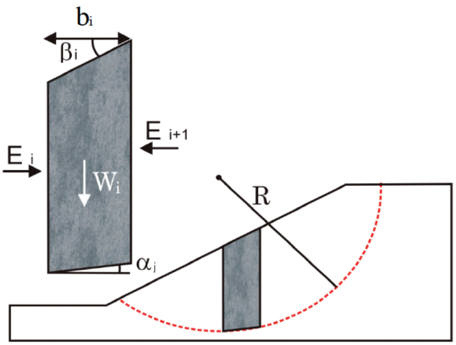
Slope stability problems are commonly analyzed using the limit equilibrium methods of slices. The limit equilibrium methods are based on determining applied stresses and mobilized strength over a trial slide surface in the soil slope, then a factor of safety is determined by considering these two quantities. Slice methods are more commonly used in limit equilibrium approach to slope stability analysis. The failing soil mass is divided into a number of vertical slices to calculate the factor of safety. The Bishop method assumes that the inter-slice forces are horizontal and inter-slice shear forces are neglected [20]. A circular slip surface is assumed in the Simplified Bishop Method. Forces considered in the Simplified Bishop method are shown in Figure 1. The resulting equilibrium equation is combined with the Mohr-Coulomb equation and the definition of the factor of safety to determine the forces on the base of the slice. Finally, moments are summed about the center of the circular slip surface to obtain the following expression for the factor of safety:

(3)

where b_i is the width of the slice, W_i is the weight of the slice. c_i and φ_i are shear parameters for the centre of the base of the slice, μ_i is pore water pressure.

Figure 1. Forces acting on a typical slice in the Simplified Bishop method.

Figure 1. Forces acting on a typical slice in the Simplified Bishop method.

In Bishop’s method the factor of safety is determined by trial and errors, using an iterative process, since the factor of safety (F_s) appears in both sides of Equation (3).

3. Estimation for Moments of the Performance Function

The first four moments ${\mu }_Z,{\mu }_Z^{\text{(2)}},{\mu }_Z^{\text{(3)}},{\mu }_Z^{\text{(4)}}$ of the performance function Z can be calculated based on the first four moments of the basic random variable X_i.

3.1. Calculation of Moments for Sample Variables

Given n samples of a random variable X_i, the sample mean μ_Xi1 and sample variance ${\sigma }_{X_i}^2$ of a random variable X_i can be calculated by Equation (4):

(4)

If we know the distribution type of a random variable X_i, ith central moment of X_i can be calculated based on the probability density function f(X_i) of X_i. The third moment μ_Xi3 and the fourth moment μ_Xi4 of X_i are calculated as follows:

(5)

The first central moment μ_X1 is zero and the second central moment is the variance ${\sigma }_X^2$. Usually the first four central moments of X_i are:

(6)

where σ_x is the standard deviation, C_sX is the skewness coefficient, C_kX is the kurtosis coefficient. Skewness and kurtosis measure the shape of a probability distribution. Table 1 gives the third and fourth central moment coefficient of several typical probability distributions. According to Table 1 we can easily calculate the third and fourth central moments.

Table 1. The third and fourth central moment coefficient.

Distribution type	Normal distribution	Lognormal distribution	Exponential distribution
Skewness coefficient CsX	0	0.324	2
Kurtosis coefficient CkX	3	3.514	9

Table 1. The third and fourth central moment coefficient.

Distribution type	Normal distribution	Lognormal distribution	Exponential distribution
Skewness coefficient CsX	0	0.324	2
Kurtosis coefficient CkX	3	3.514	9

3.2. Estimation for Moments of the Performance Function

In the present paper, Taylor series method is used in order to estimate the moments of the performance function. Let the performance function be written as Z = g(X) = g(X₁, X₂,…,X_n), the X_i terms are uncorrelated random variables. A Taylor series expansion of the performance function about the mean value gives [20]:

(7)

where

The first four moments ${\mu }_Z,{\mu }_Z^{\text{(2)}},{\mu }_Z^{\text{(3)}},{\mu }_Z^{\text{(4)}}$. of the performance function Z = g(X) can be calculated by Equation (8):

(8)

Once the four statistical moments are obtained, the PDF of g(X) can be estimated using maximum entropy method (MEM) and the probability of failure can be calculated.

4. Maximum Entropy Method for Calculation of PDF

Here the maximum entropy method is used to approximate the PDF of the performance function. The maximum entropy method is based on the concept that the distribution that maximizes the information entropy is the statistically most likely to occur. Shannon (1948) defined entropy as a measure of uncertainty about a random variable. If the level of uncertainties decreases, then the entropy decreases. The maximum of uncertainty corresponds to the maximum of entropy. For a continuous random variable, Z, the entropy is defined as:

(9)

where f(Z) denotes the probability density function of the performance function, Z, and R is the integral domain.

4.1. Optimization Formulation to Calculate PDF

Jaynes [21] formulated the maximum entropy (maxent) principle as a rational approach for choosing a consistent probability distribution, amongst all possible distribution, that contains a minimum of spurious information. The principle states that the most unbiased estimate of a probability distribution is that which maximizes the entropy subject to constraints supplied by the available information, e.g., moments of a random variable. The maximum entropy method of estimating f(Z) is stated as follows:

(10)

where μ_z is the mean value of the performance function Z, ${\mu }_Z^{\left(i\right)}$ denotes the i-th central moment of Z; m is the number of the given moment constrains. Max means that when the entropy reaches the maximum, we obtain the best probability density function. f(Z) denotes the PDF of g(X) to be determined by the maximum entropy. The optimal solution of Equation (9) is the maximum entropy estimate of f(Z).

In many studies, it was shown that the first four moments are sufficient to describe a wide range of distribution types. We use Lagrange’s method to solve for the PDF.

By introducing the Lagrange multipliers λ_i, we define the Lagrangian function:

(11)

The multiplier (λ₀ + 1) rather than λ₀ is used to give a more convenient result. This function is maximized when:

(12)

Let Equation (11) substitute into Equation (12) to lead to the analytical expression of f(Z):

(13)

where λ_i is Lagrange multiplier for the ith moment constrain. One remains to determine the values of the λ₀ and λ_i(i = 1,2,3,4). Substitute Equation (13) into Equation (10):

(14)

Then multiplying Equation (14) by e^−λ₀, one has:

(15)

which leads to the first expression required:

(16)

The second is obtained by differentiating (15) with respect to λ_i.

(17)

or:

(18)

By (10) and (13), Equation (18) reduces to the second expression:

(19)

In order to solve λ_i(i = 1,2,3,4), a set of simultaneous equations is set up. This is done by differentiating (16) with respect to λ_i.

(20)

The left-hand side of Equation (20) can be replaced by $-{\mu }_Z^{\left(i\right)}$ using Equation (19), and μ_z and ${\mu }_Z^{\left(i\right)}$ are obtained as:

(21)

(22)

For more convenient for numerical solution, Equations (21) and (22) are changed as follows:

(23)

(24)

where the R_r are the residuals that are reduced to near zero by a numerical technique. A solution can be obtained by using nonlinear programming to obtain the minimum of the sum of the squares of the residuals:

(25)

Convergence is achieved when R² < ε or |R_r| < ε, where ε is the specified acceptable error. Equation (16) is used to obtain λ₀.

Based on the probability density function f(Z), the failure probability of the slope can be calculated as:

(26)

4.2. Calculation of Failure Probability of Slope

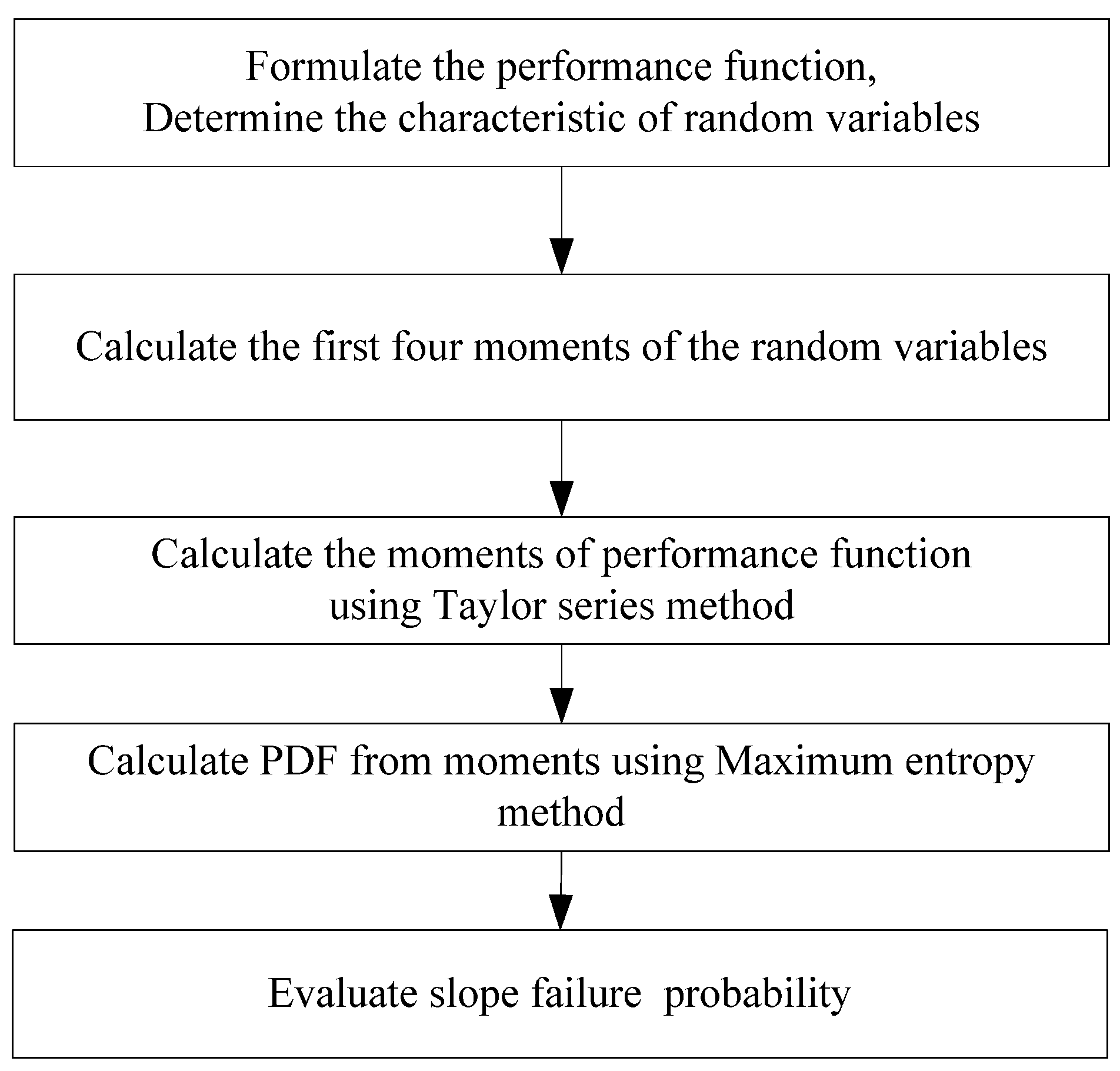
In this section, a procedure to evaluate the probability of failure based on maximum entropy method is described. The steps are as follows (Figure 2):

Figure 2. Flowchart of the proposed method.

Figure 2. Flowchart of the proposed method.

Step 1: Specify random variables and their probabilistic characteristics, and formulate the performance function for the slope stability.

Step 2: Generate random samples according to prescribed distributions and calculate the first four moments of random variables.

Step 3: Calculate the first four moments of the performance function by Taylor series method where random variables are involved.

Step 4: Estimate PDF of the performance function with Maximum entropy method.

Given the first four moments of the performance function, the Maximum entropy method is adopted to estimate the PDF subject to the moment constraints.

Step 5: Calculate the probability of failure p_f of the slope with the PDF.

5. Numerical Example

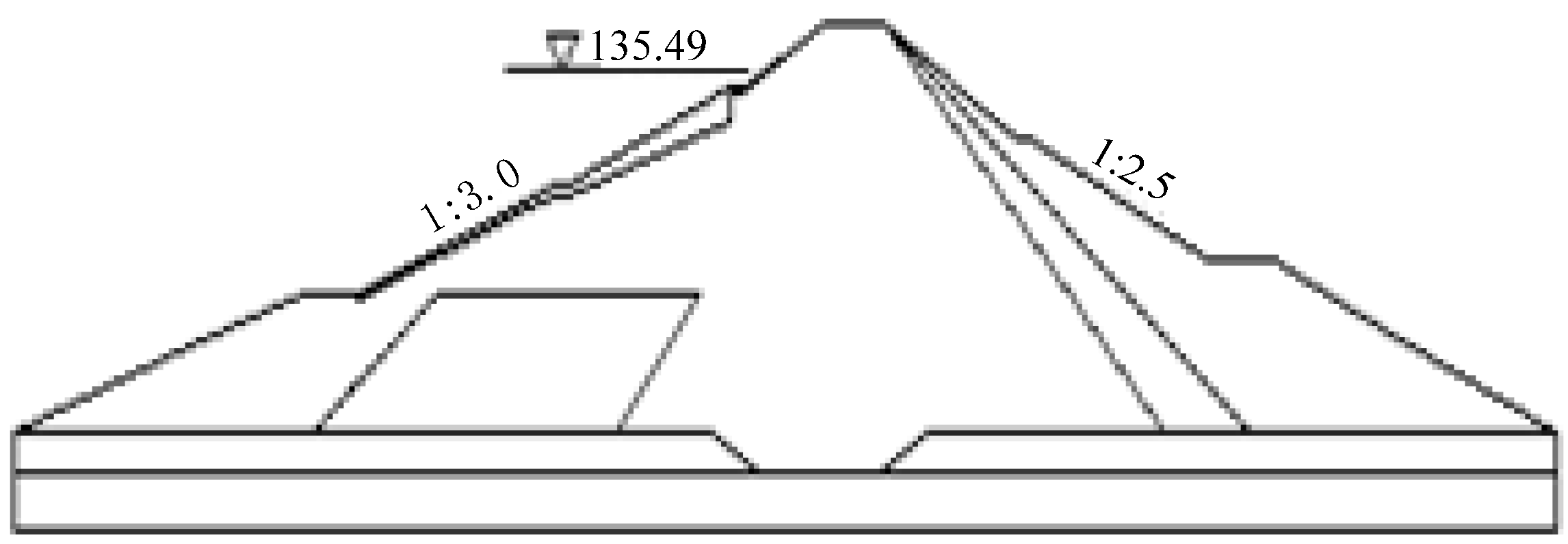
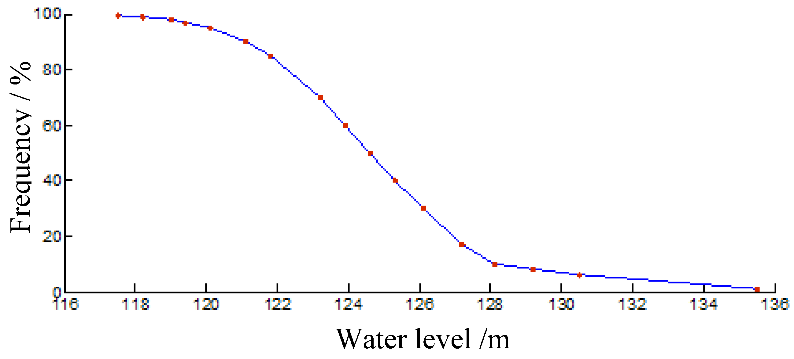
Wohushan dam is an earth-rock dam with a central clay core located in Jinan city (Shandong Province, China). This dam was selected as a case study of the developed MEM method. The dam crest elevation is 139.5 m high, the maximum dam height is 37.0 m and the dam crest length is 985 m. The normal water level is 130.5 m and the design flood level is 135.49 m. The reservoir capacity is 1.164 × 108 m³. A typical cross-section of the dam is shown in Figure 3. The water level frequency curve of Wohushan dam is shown Figure 4.

Figure 3. Typical cross-section of the Wohushan dam.

Figure 3. Typical cross-section of the Wohushan dam.

Figure 4. Water level frequency curve of the Wohushan dam.

Figure 4. Water level frequency curve of the Wohushan dam.

The basic soil parameters that are related to the stability of slope, including cohesion and friction angle, are considered as random variables. Soil parameters c and Tanφ are regarded as independent.

Term c is assumed to obey extreme type Ι distribution and Tanφ obey lognormal distribution. In addition, unit weight of dam material γ is equal to 20 kN/m³. Table 2 summarizes the statistical properties of soil parameters.

Table 2. Statistical properties of soil parameters.

Soil parameter	Distribution type	Mean value	Standard deviation
Cohesion, c (KN/m2)	Extreme type Ι	12	2.1
Internal friction coefficient , Tanφ	Lognormal	0.325	0.059

Table 2. Statistical properties of soil parameters.

Soil parameter	Distribution type	Mean value	Standard deviation
Cohesion, c (KN/m2)	Extreme type Ι	12	2.1
Internal friction coefficient , Tanφ	Lognormal	0.325	0.059

Using computer simulation software, SLOPE/W by Geoslope, the critical slip surface is first determined based on the mean value of the input parameter using Bishop methods. Probabilistic analysis is then performed on the critical slip surface, taking into consideration the variability of the input parameters. For the convenience of the analysis and calculation, Z can be transformed to the standardized form X as follows:

(27)

Where μ_z and σ_z are mean value and standard deviation of Z, respectively.

Table 3 presents the results of moments of random variables and the performance function for water level 135.5 m.

Table 3. Moments of random variables and the performance function.

Moments	Soil parameter		Performance function /Z	Standardized form / X
	c	Tanφ
0	1	1	1	1
1st	0	0	0	0
2nd	2.1	0.0594	4.819E+4	1
3rd	0	0.0217	1.520E+07	1.437
4th	0	0.0053	3.669E+09	1.580

Table 3. Moments of random variables and the performance function.

Moments	Soil parameter		Performance function /Z	Standardized form / X
	c	Tanφ
0	1	1	1	1
1st	0	0	0	0
2nd	2.1	0.0594	4.819E+4	1
3rd	0	0.0217	1.520E+07	1.437
4th	0	0.0053	3.669E+09	1.580

Let first four moments of standard random variable X substitute into Equation (28). Five Lagrange multipliers λ_i(i = 0,…,4) can be obtained by solving five nonlinear equations Equation (28).

(28)

Here the method of nonlinear least square is employed to calculate the Lagrange multipliers:

(31)

For water level 135.5 m, the probability density function (PDF) of the performance function:

(29)

when

The probability of slope failure for water level 135.5m is calculated with:

(30)

Similarly, the probability of failure for different water levels can be calculated. Table 4 shows the results of failure probability for different water levels.

Table 4. Failure probability results.

Water level/m	Minimum safety Factor	Reliability index	Failure probability/%	Risk level/10−8
117.5	1.672	3.892	0.0076
118.2	1.563	3.753	0.0112	0.516
119.0	1.537	3.694	0.0126	1.096
119.4	1.531	3.688	0.0139	1.221
120.1	1.522	3.681	0.0144	2.608
121.1	1.511	3.668	0.0157	13.845
121.8	1.504	3.653	0.0162	14.690
123.2	1.488	3.642	0.0168	15.210
123.9	1.479	3.631	0.0175	15.795
124.6	1.466	3.623	0.0188	16.705
125.3	1.459	3.614	0.0199	17.810
126.1	1.452	3.598	0.0238	20.150
127.2	1.448	3.573	0.0251	11.278
128.1	1.443	3.545	0.0278	17.063
129.2	1.437	3.521	0.0327	13.943
130.5	1.434	3.503	0.0392	6.279
135.5	1.400	3.412	0.0429	17.875
∑				186.082

Table 4. Failure probability results.

Water level/m	Minimum safety Factor	Reliability index	Failure probability/%	Risk level/10−8
117.5	1.672	3.892	0.0076
118.2	1.563	3.753	0.0112	0.516
119.0	1.537	3.694	0.0126	1.096
119.4	1.531	3.688	0.0139	1.221
120.1	1.522	3.681	0.0144	2.608
121.1	1.511	3.668	0.0157	13.845
121.8	1.504	3.653	0.0162	14.690
123.2	1.488	3.642	0.0168	15.210
123.9	1.479	3.631	0.0175	15.795
124.6	1.466	3.623	0.0188	16.705
125.3	1.459	3.614	0.0199	17.810
126.1	1.452	3.598	0.0238	20.150
127.2	1.448	3.573	0.0251	11.278
128.1	1.443	3.545	0.0278	17.063
129.2	1.437	3.521	0.0327	13.943
130.5	1.434	3.503	0.0392	6.279
135.5	1.400	3.412	0.0429	17.875
∑				186.082

Table 5 shows the results obtained from Monte Carlo method, AFOSM method (Advanced First Order Second Moment Method) and the proposed method. The result by the proposed method is close to the results very well obtained by other two methods.

Table 5. Comparison of failure probability results.

Method	Failure probability
MCS	3.85E−04
AFOSM	4.42E−04
Proposed method	4.29E−04

Table 5. Comparison of failure probability results.

Method	Failure probability
MCS	3.85E−04
AFOSM	4.42E−04
Proposed method	4.29E−04

From the perspective of computational efficiency, three methods are compared. Figure 5 shows the convergence of the simulations. The computation results indicate that 42.6 × 10⁴ reiterations is necessary for MCS method to converge but for LHS-MCS only 28.2 × 10⁴ reiterations. LHS-MC decreases the amount of calculation by 38.0%. 2.6 × 10⁴ simulations are performed to calculate the failure probabilities using the proposed method. Therefore, the Maximum-entropy method is the most efficient. As expected, considerably more trial runs are required for convergence in the case of a small probability of failure.

Figure 5. (a) Failure probability vs. simulation number with MCS method; (b) Failure probability vs. simulation number with LHS-MCS method.

Figure 5. (a) Failure probability vs. simulation number with MCS method; (b) Failure probability vs. simulation number with LHS-MCS method.

6. Conclusions

This paper presents a method to evaluate the probability of the failure of slopes using the Maximum-entropy method. The PDF of the performance function for the slope stability is calculated using the Maximum-entropy method, which is a very effective approach to construct a probability density distribution given a finite number of moments. The usefulness of this method is demonstrated by using a numerical example. Numerical results show that Maximum-entropy method can accurately predict the system probability of failure of slopes. A comparison of results from the proposed method with AFOSM and MCS confirms the accuracy of the proposed method. The proposed method is more computationally efficient than the conventional MCS and LHS-MCS methods.

References

1. Tang, W.H.; Yucemen, M.S.; Ang, A.H.-S. Probability based short term design of soil slopes. Can. Geotech. J. 1976, 13, 201–215. [Google Scholar] [CrossRef]
2. Christian, J.T.; Ladd, C.C.; Baecher, G.B. Reliability applied to slope stability analysis. J. Geotech. Eng. 1994, 120, 2180–2207. [Google Scholar] [CrossRef]
3. Hassan, A.M.; Wolff, T.F. Search algorithm for minimum reliability index of earth slopes. J. Geotech. Geoenviron. 1999, 125, 301–308. [Google Scholar] [CrossRef]
4. Low, B.K.; Tang, W.H. Reliability analysis of reinforced embankments on soft ground. Can. Geotech. J. 1997, 34, 672–685. [Google Scholar] [CrossRef]
5. Hohenbichler, M.; Gollwitzer, S.; Kruse, W.; Rackwitz, R. New light on first- and second-order reliability methods. Struct. Saf. 1987, 4, 267–284. [Google Scholar] [CrossRef]
6. Xu, B.; Low, B.K. Probabilistic stability analyses of embankments based on finite-element method. J. Geotech. Geoenviron. 2006, 132, 1444–1454. [Google Scholar] [CrossRef]
7. Greco, V.R. Efficient Monte Carlo technique for locating critical slip surface. J. Geotech. Eng. 1996, 122, 517–525. [Google Scholar] [CrossRef]
8. Papadrakakis, M.; Lagaros, N.D. Reliability-based structural optimization using neural networks and Monte Carlo simulation. Comput. Method Appl. Mech. Eng. 2002, 191, 3491–3507. [Google Scholar] [CrossRef]
9. Li, C.; Wang, S.; Wang, W. Overtopping risk analysis using LHS-MC method (in Chinese). J. Hydrol. Eng. 2012, 31, 5–9. [Google Scholar]
10. Zhao, Y.G.; Ono, T. Moment method for structural reliability. Struct. Saf. 2001, 23, 47–75. [Google Scholar] [CrossRef]
11. Lee, S.H.; Choi, H.S.; Kwak, B.M. Multilevel design of experiments for statistical moment and probability calculation. Struct. Multidiscip. Optim. 2008, 37, 57–70. [Google Scholar] [CrossRef]
12. Kiureghian, A.D.; Dakessian, T. Multiple design points in first and second-order reliability. Struct. Saf. 1998, 20, 37–49. [Google Scholar] [CrossRef]
13. Hohenbichler, M.; Rackwitz, R. Nonnormal dependent vectors in structural reliability. J. Eng. Mech. Div. 1981, 107, 1127–1238. [Google Scholar]
14. Seo, H.S.; Kwak, B.M. Efficient statistical tolerance analysis for general distributions using three-point information. Int. J. Prod. Res. 2002, 40, 931–944. [Google Scholar] [CrossRef]
15. Kang, H.Y.; Kwak, B.M. Application of maximum entropy principle for reliability-based design optimization. Struct. Multidiscip. Optim. 2009, 38, 331–346. [Google Scholar] [CrossRef]
16. Sobczyk, K.; Trebicki, J. Approximate probability distributions for stochastic systems: Maximum entropy method. Comput. Method Appl. Mech. Eng. 1999, 168, 91–111. [Google Scholar] [CrossRef]
17. Zhang, G.; Zhu, W.; Bai, S. A method of maximum entropy density function for calculation of approximate failure probability (in Chinese). Chin. J. Rock Mech. Eng. 1995, 14, 119–129. [Google Scholar]
18. Zheng, J.-J.; Xu, Z.-J.; Liu, Y. Reliability analysis for vertical bearing capacity of piles based on the maximum entropy principle (in Chinese). Chin. J. Geotech. Eng. 2010, 32, 1643–1647. [Google Scholar]
19. Bishop, A.W. The use of the slip circle in the stability analysis of earth slopes. Geotechnique 1955, 5, 7–17. [Google Scholar] [CrossRef]
20. Li, Y.; Zhao, G. Reliability analysis of structures based on maximum entropy theory (in Chinese). J. Dalian Univ. Technol. 1992, 32, 455–459. [Google Scholar]
21. Jaynes, ET. Information theory and statistical mechanics. Phys Rev. 1957, 106, 620–630. [Google Scholar] [CrossRef]