Temperature Effects, Frieden–Hawkins’ Order-Measure, and Wehrl Entropy

Abstract

We revisit the Frieden–Hawkins’ Fisher order measure with a consideration of temperature effects. To this end, we appeal to the semiclassical approach. The order-measure’s appropriateness is validated in the semiclassical realm with regard to two physical systems. Insight is thereby gained with respect to the relationships amongst semiclassical quantifiers. In particular, it is seen that Wehrl’s entropy is as good a disorder indicator as the Frieden–Hawkins’ one.

1. Introduction

In this work we apply the Frieden–Hawkins (FH) notion of order [1] to the semiclassical realm, an important component of our current physical understanding of the world [2,3]. It will be seen in this way that semiclassical order-considerations allow one to obtain a different (from the usual) perspective regarding different semiclassical quantifiers and to gain some insight into their individual roles, uncovering novel relations amongst them. As a physical background, we have in mind in this paper the harmonic oscillator (HO) and the Kerr effect. After reviewing some introductory concepts, we will present our communication’s contributions, in which a main ingredient is temperature T. Why? Because in previous FH-works the temperature-concept was not considered. This contribution deals with the order-concept in two semiclassical scenarios: (a) smoothing of Wigner’s harmonic-oscillator phase-space function and (b) molecular-aligning Kerr-interaction. Accordingly,

• We begin our considerations in Section 2 by sketching basic notions regarding Frieden–Hawkins’ order measure.
• In Section 3 we do a similar introductory exposition to basic semiclassical ideas, which is necessary because we will compare/assess the Frieden–Hawkins order-concept with semiclassical quantifiers. After these somewhat lengthy preparations, we develop our present ideas and results.
• In Section 4 we investigate order with reference to the process of coarse-graining, as applied to the Wigner function.
• In Section 5 we revisit again the FH order notion, this time with regard to the Kerr effect.
• Finally, some conclusions are drawn in Section 6.

2. Frieden–Hawkins Order Measure: A Brief Review

Order is a necessary condition for anything the human mind may be able to grasp. Any type of arrangement, such as a display of commodities offered for sale, an inventory, or an oral presentation, is deemed orderly when observers are able to understand the concomitant overall structure. A significant statement on the behavior of Nature, the Second Law of Thermodynamics, states that the world moves from orderly states to an ever-increasing disorder. One may cite Planck (in 1920) “... it is not the atomic distribution, but rather the hypothesis of elementary disorder, which forms the real kernel of the principle of increase of entropy and, therefore, the preliminary condition for the existence of entropy. “Without elementary disorder there is neither entropy nor irreversible processes” [4]. Accordingly, the notion of disorder, as measured by an entropic quantifier H, is well established in the literature.

Consider a complementary concept: that of “level of order”, or just order, in a continuous system described by the probability density p(x). The word itself is rarely quantified in mathematical fashion, as was the case with the vocable “information” before Shannon. What do we mean by a continuous system’s order? Several authors have analyzed this question à la Planck, i.e., via the second law of thermodynamics: “disorder must increase” and, consequently, order must decrease, where order is in some sense the “opposite” of disorder. However, to attempt to define a physical effect as being simply the opposite of some other effect cannot succeed, since the vocable “opposite” does not have a unique meaning. Frieden and Hawkins ask, with reference to the entropy H, if we are here speaking of its negative (the “negentropy”, see below) −H, or of its reciprocal 1/H, or the function exp(−H) or …? As a way out of the conundrum, they note that all physical concepts are defined by distinct physical effects. For example, the concept of entropy arises as the measure that obeys the second law of thermodynamics. The notion of order should likewise be defined by its own physical effect. What would that effect be? A clue emerges by considering a discrete system, characterized by a probability law P_i, i = 1,…N, with discrete states i. There the measure of order is indeed the “negentropy”:

$${\mathcal{R}}_H\equiv +{\displaystyle \sum _{i=1}^N}{P}_{i}log{P}_i$$

(1)

This quantifier satisfies the no-increasing tenet after any regrouping of its finest microstates into larger (coarser) macrostates. Such regrouping is precisely the physical operation defining the measure. However, the probability density p(x) above is continuous, not discrete. A form of the measure Equation (1) valid for continuous probability densities can be formally obtained by replacing the sum in Equation (1) with an integral over the relevant configuration or phase space. Even if this new version of Equation (1) plays a central role in several important scenarios (ranging from Boltzmann’s celebrated interpretation of the second law of thermodynamics via his H-theorem [5], to Jaynes’ maximum entropy principle and its multiple applications [6]), it is well-known that, to some extent, it is conceptually problematic. If one tries to “connect” the discrete and the continuous versions of Equation (1) via a discretization of the continuous phase space, one immediately runs into problems, because the concomitant continuous limit P_i → p(x)dx of the measure is not well-defined since log dx → −∞. In a related vein, note the somehow “disturbing” fact that the continuous version of Equation (1) does not have a definite sign: for some probability densities it adopts a positive value, while for others its value is negative. An important point of the present communication is that these problems do not arise in the semiclassical realm, as we shall see below.

Still another limitation of Equation (1) is encountered in its actual use. Its application for treating systems that are not in states at or near thermodynamic equilibrium has been questioned. Of course, several important systems found in nature are not of this kind (see [7,8] for comprehensive and interesting recent discussions of the inadequacy of Equation (1) for the description of several out of equilibrium scenarios). Examples are very rarefied gases, where molecular collisions are infrequent, or systems of interacting fermions at very low temperature, where dissipative processes become ineffective. Last but certainly not least, there are “living” systems [9]. These constitute the most important and most complex systems far from equilibrium. Living systems, in fact, die at thermodynamic equilibrium!

Is there any measure that works regardless of how far the system’s state is from its equilibrium state? For a didactic discussion of the (affirmative) answer see [10]. The regrouping process described above is to be regarded as a special case (the discrete counterpart) of a generally continuous physical process called “coarse graining” (see below for details [1,10,11,12]).

2.1. Coarse Graining

A coarse-grained description refers to an explication in which the finest details are either smoothed over or averaged out, with a significant diminution of resolution. Accordingly, a coarse-grained description of a system limits itself to the grosser subcomponents. In [1,10,11,12] the order notion is defined based on such kind of regrouping processes (regrouping order (RO)).

As an RO example, consider cases in which random noise from a generally shaped distribution p(n) degrades the system, producing a wider, smoother density law that is the convolution of p(x) and p(n) This process “coarsens” the granular nature of the system’s density law p(x). If p(x) corresponds to a photographic picture, it would experience an increased grain size. Note the RO notion is broader than that pertaining to measure Equation (1), since the latter does not include the possibility of added noise from a generally shaped noise distribution p(n). Regrouping discrete states is roughly equivalent to convolution with a rectangle function [10].

2.2. Fisher Order Measure

In recent efforts [1,11,12], a mathematical form for order was found from first principles, on the basis of coarse graining the system. Fisher’s information measure (FIM) I [1] is a fundamental part of the answer. Frieden and Hawkins define an order ${\mathcal{R}}^{\prime }$ as:

$${\mathcal{R}}^{\prime }\equiv 8^{-1}{L}^{2}I$$

(2)

where I is defined in terms of a probability distribution function p(x) [13]:

$$I={\int }_{-\infty }^{\infty }\mathrm{d}\mathrm{x}p(x){\left(\frac{\mathrm{d}lnp(x)}{\mathrm{d}x}\right)}^2$$

(3)

vis-Ã -vis Equation (1), Fisher’s order measure does apply for continuous distributions, regardless of how far the system’s state is from equilibrium. Fisher’s order measure is defined for a general state of a system. Parameter L is the maximum chord length connecting two surface points of the system.

Fisher’s information derives uniquely from the single physical requirement: after the continuous distribution p(x) is coarse grained (see previous subsection), its order ${\mathcal{R}}^{\prime }$ may not increase. That is:

$$\Delta {\mathcal{R}}^{\prime }\le 0\mathrm{for}\Delta t>0$$

(4)

Processes of coarse graining are the essence in the Frieden–Hawkins’ order definition. The process is described in the preceding subsection and more details are given in Section 4 below. This coarse graining takes place over the small time interval Δt. Moreover, in contrast with the near-equilibrium state assumed in using Equation (1), our probability distribution function p(x) is regarded as describing a general state, not necessarily at or near thermodynamic equilibrium. Order-measure Equation (2) was derived for a one dimensional system in [1], and extended to any K dimensional system in [11]. For the sake of convenience, from now on we will use a scaled version of ${\mathcal{R}}^{\prime }$, to be called $\mathcal{R}$, that turns out to be identical to I:

$$\mathcal{R}=8L^{-2}{\mathcal{R}}^{\prime }\equiv I$$

(5)

Thus, our rescaled FIM and FH-order become equivalent quantities.

2.3. Some Features of the Frieden–Hawkins Order Measure

The present order-measure Equation (2)

• is dimensionless (neither length, nor time, nor mass), which has the benefit of allowing completely different phenomena to be compared for their levels of order;
• is invariant under uniform stretching x_k → a_kx_k, k = 1, …, K, with the a_k = constants; and
• measures the number of ordered “details” within the system, rather than their density of structure—e.g., for a one dimensional system p(x) = (2/a) sin²(nπx/a), 0 ≤ x ≤ a the order $ℛ$ = 4π²n² This is independent of the system extension a and, instead, is purely a rapidly increasing function of the total number n of sinusoidal waves within the system.

This is in the spirit of the well-known Kolmogorov–Chaitin complexity measure [14,15], which is given by the minimum length of the computer program, or the shortest description in some fixed universal language, required to generate or to characterize a string of numbers. Summing-up, we require a good measure of order (disorder) to be:

• dimensionless (no length, time, mass);
• translationally invariant;
• dependent on the number of details.

2.4. Previous FH-applications

In [11] Fisher’s order measure ${\mathcal{R}}^{\prime }$ was used to predict that a rod-like living creature such as an E. coli bacterium can be compressed into a disc-like shape with the same level of order, provided it undergoes mitosis while being deformed. This prediction was independently confirmed experimentally by another group (see [11] for details). It allows, e.g., life to exist and evolve even under great compression such as deep into the earth.

In a recent application to cosmology, it was found that, contrary to intuition, the Hubble expansion per se does not imply an order-decrease [12]. We are speaking of ${\mathcal{R}}^{\prime }$ for the mass-density in a Robertson–Walker universe. This is described by the metric:

$$\mathrm{d}{s}^2={(c\mathrm{d}t)}^2-a^2(t)(\mathrm{d}{x}^2+\mathrm{d}{y}^2+\mathrm{d}{z}^2),(x,y,z)\equiv \mathbf{r}$$

(6)

Fisher’s order measure is, for such a universe, invariant. We emphasize that this invariance refers only to expansion-effects, without taking into account the interaction between the different elements of mass. Finally, in [10] it is shown that the FH-order of space is a purely geometrical property that depends only on distances and not on other matter-energy properties.

The role of temperature in the present context is yet to be discussed. We intend to remedy such circumstance here.

3. The Semiclassical Approach

The semiclassical approach has a long and distinguished history and is still a very important weapon in the physics’ armory. Indeed, semiclassical approximations to quantum mechanics remain an indispensable tool in many areas of physics and chemistry. Despite the extraordinary evolution of computer technology in the last years, an exact numerical solution of the Schrödinger equation is still quite difficult for problems with more than a few degrees of freedom. Another great advantage of the semiclassical approximation lies in that it facilitates an intuitive understanding of the underlying physics, which is usually hidden in blind, brute force numerical solutions of the Schrödinger equation. Although semiclassical mechanics is as old as the quantum theory itself, the field is continuously evolving. There still exist many open problems in the mathematical aspects of the approximation as well as in the quest for new effective ways to apply the approximation to various physical systems (see, for instance [2,3] and references therein). In this work we focus attention upon statistical scenarios at finite temperature and establish what we believe are interesting connections between semiclassical probability distributions at finite temperature and information theory regarding the notion of “order” (see below). Even if some (not all!) of our considerations revolve around the harmonic oscillator, this is such an important system that HO insights usually have a wide impact, as the HO constitutes much more than a mere example. Nowadays it is of particular interest for the dynamics of bosonic or fermionic atoms contained in magnetic traps [16,17,18] as well as for any system that exhibits an equidistant level spacing in the vicinity of the ground state, like nuclei or Luttinger liquids.

3.1. Semiclassical Quantifiers

We briefly review below the main semiclassical quantifiers.

3.1.1. Wigner’s Distribution

In a semiclassical context the Wigner quasi-probability distribution A_w(x, p) (also called the Wigner function or the Wigner–Ville distribution) acquires paramount significance. It is a special type of quasi-probability distribution. It was introduced by Eugene Wigner in 1932 [19] to study quantum corrections to classical statistical mechanics. In trying to approximate it, in some fashion one is prone to fall into the semiclassical domain. The goal was to supplant the wave-function that appears in Schrödinger’s equation with a probability distribution in phase space that is a generating function for all spatial autocorrelation functions of a given quantum-mechanical wave-function ψ(x). Thus, in the map between real phase-space functions and Hermitian operators introduced by Weyl in 1927, A_w maps on the quantum density matrix [20]. One speaks of the Weyl–Wigner transform of the density matrix. In 1949 Moyal [21], who had also re-derived it independently, recognized A_w as the quantum moment-generating functional, i.e., as the basis of an elegant encoding of all quantum expectation values, and hence quantum mechanics in phase space (Weyl quantization). It has applications in statistical mechanics, quantum chemistry, quantum optics, classical optics and signal analysis in diverse fields such as electrical engineering, seismology, biology, speech processing, and engine design [22]. Thus, Wigner’s is the most elaborate phase-space (PS) formulation of quantum mechanics [19,23,24]. Specifically, the effects of order ℏ² are included in A_w [25,26]. To every quantum state a PS function (A_w) can be assigned. This PS function can, regrettably enough, assume negative values so that a probabilistic interpretation becomes questionable.

3.1.2. Husimi’s Distribution

The above-mentioned limitation was overcome by Husimi [27] (among others). The Husimi distribution is a quite useful mathematical tool, very much applied in different contexts [27,28,29]. It is a probability distribution commonly used to represent the quantum state of light. It is often employed in the field of quantum optics and particularly for tomographic purposes, and includes quantal effects up to order ℏ [26]. It is usually built up employing coherent states |z〉 on the basis of phase space coordinates x, p, with $z=(1/\sqrt{2\hslash })(x+ip)$. The Husimi probability distributions μ(x, p) (see definition in next Subsection), with $\widehat{\rho }$ the density matrix, can be regarded as a “coarse-grained Wigner distribution” [23], and the whole of quantum mechanics can be completely reformulated in Husimi-terms [28,30,31,32]. Indeed, μ(x, p) is a Wigner–distribution A_w(x, p), smeared over an ℏ sized region of phase-space [33]. The smearing renders μ(x, p) a positive function, even if A_w does not have such a character, the μ distribution referring to a special type of probability: that for simultaneous but approximate location of position and momentum in phase space [33].

Remark that the Wigner function displays large oscillations and may adopt negative values that make it a quasi-distribution rather than a classical probability density. On a compact phase space of area A it is able to reveal fine structures on a sub-Planck scale of order ${\hslash }^2/A$ [34], structures that can be traced to quantum interferences from distant localized objects [34,35,36,37], which in turn enhance the state’s sensitivity to perturbations [34,35,36,37]. Instead, the Husimi distribution, just a Gaussian coarse graining of the Wigner function on an area of size ℏ, washes out the negative part, and it is hence suitable as a probability density [38]. However, such smoothing may hide significant important attributes or aspects of the Wigner function [39]. Summing up, while the Wigner function exhibits high resolution, it is not free of long-range quantum interferences. The Husimi distribution washes out quantum interferences at the price of hiding important semiclassical structures [39].

3.1.3. Wehrl Entropy

The paradigmatic semiclassical entropic quantifier is that of Wehrl’s entropy W [40], which is built up using coherent states [33,40,41]. The pertinent definition reads:

$$W=-\int \frac{{\mathrm{d}}^{2}z}{\pi }\mu (z)ln\mu (z)$$

(7)

where $\mu (z)=\langle z\left|\widehat{\rho }\right|z\rangle$ is the Husimi distribution [27,33,41,42], which is normalized to unity according to $\int ({\mathrm{d}}^{2}z/\pi )\mu (z)=1$, with ${\mathrm{d}}^{2}z=\mathrm{d}x\mathrm{d}p/2\hslash$ and $z={(mw/2\hslash )}^{1/2}x+\mathrm{i}{(2\hslash m\omega )}^{1/2}p$. The uncertainty principle manifests itself through the inequality W ≥ 1, which was first conjectured by Wehrl [40] and later proved by Lieb (see, for instance [33]).

The usual treatment of equilibrium in statistical mechanics makes use of the Gibbs’s canonical distribution, whose associated, thermal density matrix is given by $\widehat{\rho }=Z^{-1}{e}^{-\beta \widehat{H}}$, with $Z=\mathrm{Tr}(e^{-\beta \widehat{H}})$ the partition function, $\beta =1/k_{B}T$ the inverse temperature T, and $k_B$ the Boltzmann constant. In order to conveniently write down an expression for W, consider an arbitrary Hamiltonian $\widehat{H}$ of eigen-energies $E_n$ and eigenstates $|n\rangle$ (n stands for a collection of all the pertinent quantum numbers required to label the states). One can always write [33]:

$$\mu (z)=\frac{1}{Z}\sum _n{e}^{-\beta E_n}{\left|\langle z|n\rangle \right|}^2$$

(8)

A useful route to W starts then with Equation (8) and continues with Equation (7). In the special case of the harmonic oscillator the coherent states are of the form [41]:

$$|z\rangle =e^{-{\left|z\right|}^2/2}\sum _{n=0}^{\infty }\frac{z^n}{\sqrt{n!}}|n\rangle$$

(9)

where $|n\rangle$ are a complete orthonormal set of eigenstates and whose spectrum of energy is $E_n=(n+1/2)\hslash \omega$, $n=0,1,\dots$ In this situation we have the useful analytic expressions obtained in [33]:

$${\mu }_{HO}(z)=(1-e^{-\beta \hslash \omega })e^{-(1-e^{-\beta \hslash \omega }){\left|z\right|}^2}$$

(10)

$$W_{HO}=1-ln(1-e^{-\beta \hslash \omega })$$

(11)

When T → 0, the entropy takes its minimum value $W_{HO}=1$, expressing purely quantum fluctuations. On the other hand when $T\to \infty$, the entropy tends to the value $-ln(\beta \hslash \omega )$ that expresses purely thermal fluctuations [33].

Looking back at the main features of a good measure of order (disorder) (Section 2.3), we see that its features also characterize Wehrl’s entropy as a measure of disorder. The first two characteristics are evident. As for the third one, notice the dependence on ω, which makes W to diminish when the frequency increases.

3.1.4. Semiclassical Fisher Information

The Fisher’s information measure can be defined as the variance of the score, or as the expected value of the observed information. The role of the Fisher information in the asymptotic theory of maximum-likelihood estimation was emphasized by the statistician Sir Ronald Fisher in the 1920s. FIM is also used in Bayesian statistics [13].

In particular, it is possible to define the Fisher measure in a semiclassical context. For details and an exhaustive analysis one can consult [43,44]. As a particular instance, we mention here the FIMs associated to the Wigner and Husimi distributions for the harmonic oscillator, which reads [45]:

$$I_{w,h}=\frac{1}{4}\int \frac{{\mathrm{d}}^{2}z}{\pi }{A}_{w,h}(z){\left(\frac{\partial ln{A}_{w,h}(z)}{\partial \left|z\right|}\right)}^2$$

(12)

where we stand for $A_w(z)=2tanh(\beta \hslash \omega /2)e^{-{2tanh(\beta \hslash \omega /2)\left|z\right|}^2}$ the Wigner distribution function of the harmonic oscillator and, $A_h(z)\equiv \mu (z)$ the Husimi distribution (10). Integrating over phase space, for an HO of frequency ω at the temperature T, we find the Fisher measure associated to the Wigner and Husimi distributions, respectively [46]:

$$I_w=2tanh(\beta \hslash \omega /2)$$

(13)

and,

$$I_h=1-e^{-\beta \hslash \omega }$$

(14)

We saw that the Husimi distribution is a Gaussian coarse graining of the Wigner function on an area of size ℏ [26]. Also, we can recast the phase space FIMs for the Wigner and Husimi functions as, respectively:

$$A_w(z)=I_w{e}^{-I_w{\left|z\right|}^2}$$

(15)

$$A_h(z)=I_h{e}^{-I_h{\left|z\right|}^2}$$

(16)

expressions that show that the semiclassical distributions depend exclusively on the appropriate FIMs.

4. Order and Coarse-Graining

We start here presenting our semiclassical, novel Frieden–Hawkins considerations, based on the findings of [47]. Keep Equation (5) in mind! The coarse graining process described above, which is the basis for introducing the FH order measure, is now applied to the HO-Wigner function, a procedure that generates a family of semiclassical quantifiers. The Wigner description is exact. The coarse-graining produces approximations of varying exactitude that diminishes as the degree of smearing becomes larger. We assimilate here the exactitude to “most-ordered”. As we lose exactitude, disorder increases.

Consider the two bi-dimensional phase-space variables (x, p) and (X, P), and write:

$${\left|z\right|}^2\equiv z^2=\frac{1}{2\hslash }\left(m\omega x^2+\frac{p^2}{m\omega }\right)$$

(17)

with a similar expression for a $Z-$linear combination (we must replace x, p, and z by X, P, and Z, respectively).

We appeal to the normalized kernel:

$$G(z-Z)=\frac{z^{-1}}{\xi }{e}^{-(1/\xi ){(z-Z)}^2}$$

(18)

where ξ a real non-negative parameter that characterizes the coarse graining’s degree. We apply it to the phase-space harmonic oscillator-Wigner function $A_w(z)=I_w{e}^{-I_w{\left|z\right|}^2}$ [19,45]. Normalization is provided via:

$$\int \frac{{\mathrm{d}}^{2}z}{\pi }G(z-Z)=1;\int \frac{{\mathrm{d}}^{2}z}{\pi }{A}_w(z)=1$$

(19)

Our objective now is to coarse-grain $A_w(z)$ via smoothing and get an approximate phase-space descriptor $A_{\xi }(Z)$:

$$A_{\xi }(Z)=\int \frac{{\mathrm{d}}^{2}z}{\pi }G(z-Z)A_w(z)$$

(20)

Setting $b=1/\xi$ and introducing auxiliary quantities $\mu =b{I}_w,\gamma =I_w+b$ it is possible to obtain [47]:

$$A_{\xi }(Z)=\frac{I_w}{\xi I_w+1}{e}^{-\frac{I_w}{\xi I_w+1}{Z}^2}$$

(21)

For effective coarse-graining we require $I_w/(\xi I_w+1)<I_w$. This implies $\xi \ge 0$ [47]. The coarse-graining parameter ξ quantifies the degree of disorder we wish to introduce. The $\xi -$coarse-grained Fisher measure then becomes [47]:

$${\mathcal{R}}_{\xi }\equiv I_{\xi }=\frac{I_w}{\xi I_w+1}=\frac{{\mathcal{R}}_w}{\xi {\mathcal{R}}_w+1}$$

(22)

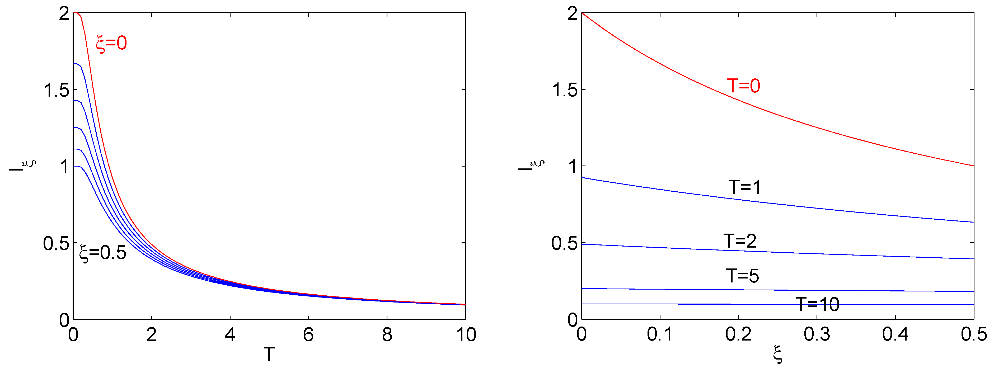
The order ${\mathcal{R}}_{\xi }$ steadily diminishes as ξ grows from 0 to $1/2$, with $0\le {\mathcal{R}}_{\xi }\le 2$. In particular, $\xi =1/2$ yields the Husimi distribution, and $\xi =0$ to the Wigner [47]. We depict in Figure 1 ${\mathcal{R}}_{\xi }=I_{\xi }$ vs. ξ for different temperatures. It is clearly seen that the Fisher-measure, i.e., order ${\mathcal{R}}_{\xi }$, diminishes with both T and ξ. Figure 2 depicts the same effect, now plotting $I_{\xi }={\mathcal{R}}_{\xi }$ vs. T for different coarse-graining parameters. The same effect reported above becomes evident. Summing up, the larger ξ, the larger the amount of coarse graining. Thus, we reconfirm, in semiclassical fashion, the connection between the notions of order on the one hand, and the Fisher-quantifier on the other hand, postulated by Frieden and Hawkins.

Figure 1. HO-smoothing. FH-order ${\mathcal{R}}_{\xi }=I_{\xi }$ as a function of ξ for different temperatures T (right) and vs. T for different ξ (left).

Figure 1. HO-smoothing. FH-order ${\mathcal{R}}_{\xi }=I_{\xi }$ as a function of ξ for different temperatures T (right) and vs. T for different ξ (left).

Figure 2. HO-smoothing. FH-order in the $\xi -T$ plane. Ordered situation lies at the southwest corner and decreases as we move away from it.

Figure 2. HO-smoothing. FH-order in the $\xi -T$ plane. Ordered situation lies at the southwest corner and decreases as we move away from it.

We pass now to calculate the semiclassical entropy associated to the coarse-grained Wigner’s probability distribution $A_{\xi }$ given by Equation (21). We deal with:

$$S_{\xi }=-\int \frac{{\mathrm{d}}^{2}z}{\pi }{A}_{\xi }(z)ln{A}_{\xi }(z)$$

(23)

Thus, replacing Equation (21) into the above expression and integrating over phase space we obtain:

$$S_{\xi }=S_w+ln(1+\xi I_w)$$

(24)

where $S_w=1-ln{I}_w$ is the Shannon entropy associated to the Wigner’s function and $I_w$ is given by Equation (13). We easily verify that for $\xi =1/2$ we recover the Wehrl entropy as follows:

$$S_{1/2}=1-ln{I}_w+ln(1+I_w/2)$$

(25)

and after a bit of algebra and trigonometry we finally arrive at:

$$S_{1/2}\equiv W$$

(26)

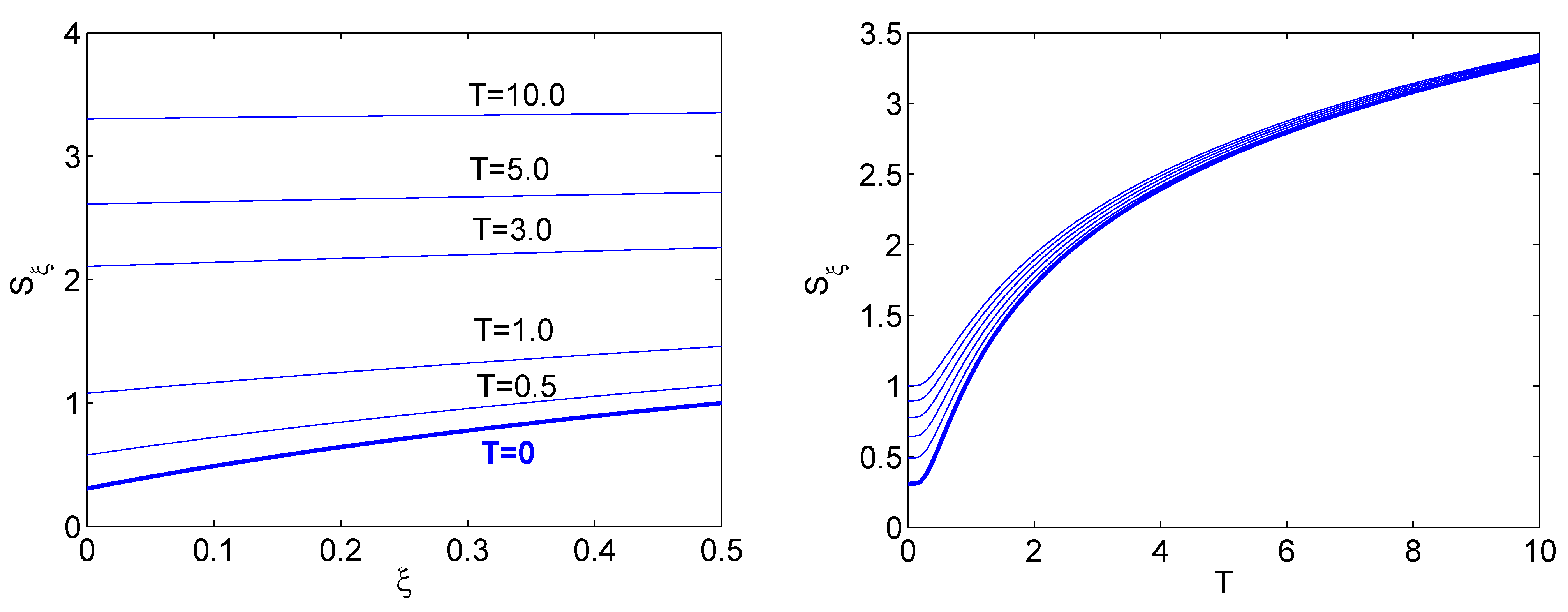
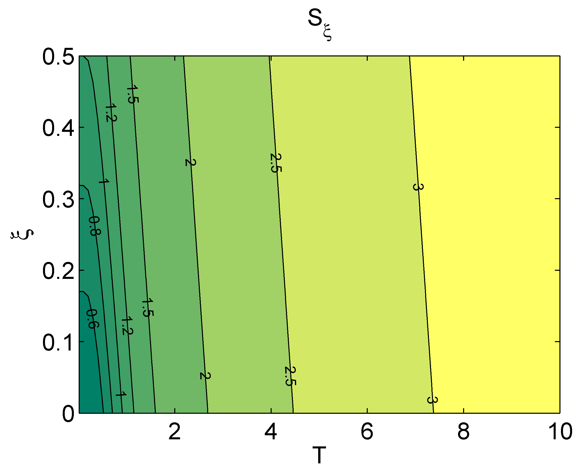
We display below in Figure (3) and in Figure (4) the $S_{\xi }$-behavior in three graphs. It is immediately appreciated that entropic disorder complies with Section (2.3)-tenets for an order/disorder measure.

Figure 3. HO-smoothing. $S_{\xi }$ as a function of ξ for different temperatures T (right) and vs. T for different ξ (left).

Figure 3. HO-smoothing. $S_{\xi }$ as a function of ξ for different temperatures T (right) and vs. T for different ξ (left).

Figure 4. HO-smoothing. Entropy $S_{\xi }$ in the plane ξ-T. Order lies at the southwest corner and disorder grows as one moves away from it. The sequence of different colors shows that the entropy appropriately represents disorder.

Figure 4. HO-smoothing. Entropy $S_{\xi }$ in the plane ξ-T. Order lies at the southwest corner and disorder grows as one moves away from it. The sequence of different colors shows that the entropy appropriately represents disorder.

5. Kerr Effect

As an important physical ingredient of this presentation, we focus attention upon the Kerr effect, also called the quadratic electro-optic effect, discovered in 1875 by the Scottish physicist John Kerr. It refers to a change in the refractive index of a material in response to an applied electric field. All materials show a Kerr effect, but certain liquids display it more strongly than others. The difference in index of refraction, $\Delta n$, is given by:

$$\Delta n=\lambda K{\mathcal{E}}^2$$

where λ is the wavelength of the light, K the so-called Kerr constant, and $\mathcal{E}$ is the strength of the electric field. The optical Kerr effect manifests itself temporally as self-phase modulation, a self-induced phase- and frequency-shift of a pulse of light as it travels through a medium. This process, along with dispersion, can produce optical solitons. In materials with high Kerr constants the molecules will tend to align with the applied electric field [48]. Thus, “order” can be said to augment. The Hamiltonian for this system is:

$${\widehat{H}}_k=\hslash \omega \left({\widehat{a}}^{†}\widehat{a}+\frac{1}{2}\right)+\hslash \chi {({\widehat{a}}^{†})}^2{(\widehat{a})}^2$$

(27)

where the nonlinear coupling coefficient χ is related to the Kerr medium third-order susceptibility [48]. In a number-state basis, the so-called Kerr states are eigenstates of the Hamiltonian ${\widehat{H}}_k$, and are defined as [49]:

$$|{\Psi }_k\rangle =e^{-{\left|z\right|}^2/2}\sum _{n=0}^{\infty }\frac{z^n}{{(n!)}^{1/2}}{e}^{i\gamma n(n-1)/2}|n\rangle$$

(28)

with $\gamma =2\chi L/v$, where L is the length of the Kerr medium and v the appropriate phase velocity inside the medium [49].

5.1. Husimi Distribution, Wehrl Entropy and FH-order for a Kerr Medium

By recourse to semiclassical probability distribution, we wish to investigate now the concept of order enunciated in previous sections. For such purpose, we employ here a simple model that hopefully will be able to shed some lights on the matter. Let us rewrite the Kerr–Hamiltonian in terms of the number operator $\widehat{n}={\widehat{a}}^{†}\widehat{a}$:

$${\widehat{H}}_k=\hslash \omega (\widehat{n}+1/2)+\hslash \chi ({\widehat{n}}^2-\widehat{n})$$

(29)

The anharmonic parameter χ is a positive real quantity that characterizes the Kerr environment. Our study is based on the construction of the Husimi distribution according to:

$${\mu }_k(z)=\langle {\Psi }_k|\widehat{\rho }|{\Psi }_k\rangle$$

(30)

with (i) $|{\Psi }_k\rangle$ being coherent states Equation (28) and (ii) $\widehat{\rho }=e^{-\beta {\widehat{H}}_k}/Z_{Kerr}$ the system’s density matrix of the Kerr medium. Of course, $Z_{Kerr}=\mathrm{Tr}{e}^{-\beta {\widehat{H}}_k}$ is the partition function. Replacing the form of $Z_{Kerr}$ into Equation (30) we are led to:

$${\mu }_k(z)=e^{-{\left|z\right|}^2}\frac{{\sum }_{n=0}^{\infty }{e}^{-\beta \hslash (\omega -\chi )n}{e}^{-\beta \hslash \chi n^2}{\left|z\right|}^{2n}/n!}{{\sum }_{n=0}^{\infty }{e}^{-\beta \hslash (\omega -\chi )n}{e}^{-\beta \hslash \chi n^2}}$$

(31)

Additionally, it is easy to ascertain that the Wehrl entropy is of the form Equation (7) with the Husimi distribution given by Equation (31).

The semiclassical FH-order (or Fisher information) for the Kerr medium is defined as [50]:

$$I=\frac{1}{4}\int \frac{{\mathrm{d}}^{2}z}{\pi }{\mu }_k(z){\left(\frac{\partial ln{\mu }_k(z)}{\partial \left|z\right|}\right)}^2.$$

(32)

In the limit $\chi \to \infty$, the Husimi function (31) tends to ${\mu }_k{(z)}^{(\infty )}=e^{-{\left|z\right|}^2}$. Replacing this in Fisher measure and Wehrl entropy, we respectively obtain:

$$I=\frac{1}{4}\int \frac{{\mathrm{d}}^{2}z}{\pi }{\mu }_k{(z)}^{(\infty )}{\left(\frac{\partial ln{\mu }_k{(z)}^{(\infty )}}{\partial \left|z\right|}\right)}^2$$

(33)

i.e.,

$$I=2{\int }_0^{\infty }\mathrm{d}z{\left|z\right|}^3{e}^{-{\left|z\right|}^2}=1$$

(34)

and,

$$W=-\int \frac{{\mathrm{d}}^{2}z}{\pi }{\mu }_k{(z)}^{(\infty )}ln{\mu }_k{(z)}^{(\infty )}$$

(35)

i.e.,

$$W=2{\int }_0^{\infty }\mathrm{d}z{\left|z\right|}^3{e}^{-{\left|z\right|}^2}=1$$

(36)

Thus, for χ tending to infinity, we find the surprising result that Wehrl entropy and Fisher information coincide! This does not happen for Shannon’s entropy. The reason is the Lieb-bound $W\ge 1,$ which reflects the uncertainty principle effect. Since unity is the highest possible value that Fisher’s information can reach, the above coincidence ensues.

In Figure 5 we plot the Wehrl entropy W and the FH-order (FIM) vs. T. Of course, order decreases and the entropy increases. Per contra, Wehrl’s entropy decreases and order increases for growing χ, because the Kerr effects promotes an “ordering” in the system via molecular alignment with an external electric field. Of course, temperature growth works against this ordering effect.

Figure 5. Kerr medium. Left plot: FH-order I (blue lines) and Wehrl entropy (red lines) measures vs. T for different χ-values. Thick lines indicate χ = 0 while thin lines correspond to, respectively, χ = 0.1, 0.3, 0.5, 0.7, 1.0, 1.5, and 3; Right plot: FH-order I (blue lines) and Wehrl entropy (red lines) measures vs. χ for different T-values. For T = 0 one has W = I = 1 (black thick line). Thin lines correspond (from inside outwards) to, respectively, T = 0.5, 1.0, 2.0, 3.0, and 5.

Figure 5. Kerr medium. Left plot: FH-order I (blue lines) and Wehrl entropy (red lines) measures vs. T for different χ-values. Thick lines indicate χ = 0 while thin lines correspond to, respectively, χ = 0.1, 0.3, 0.5, 0.7, 1.0, 1.5, and 3; Right plot: FH-order I (blue lines) and Wehrl entropy (red lines) measures vs. χ for different T-values. For T = 0 one has W = I = 1 (black thick line). Thin lines correspond (from inside outwards) to, respectively, T = 0.5, 1.0, 2.0, 3.0, and 5.

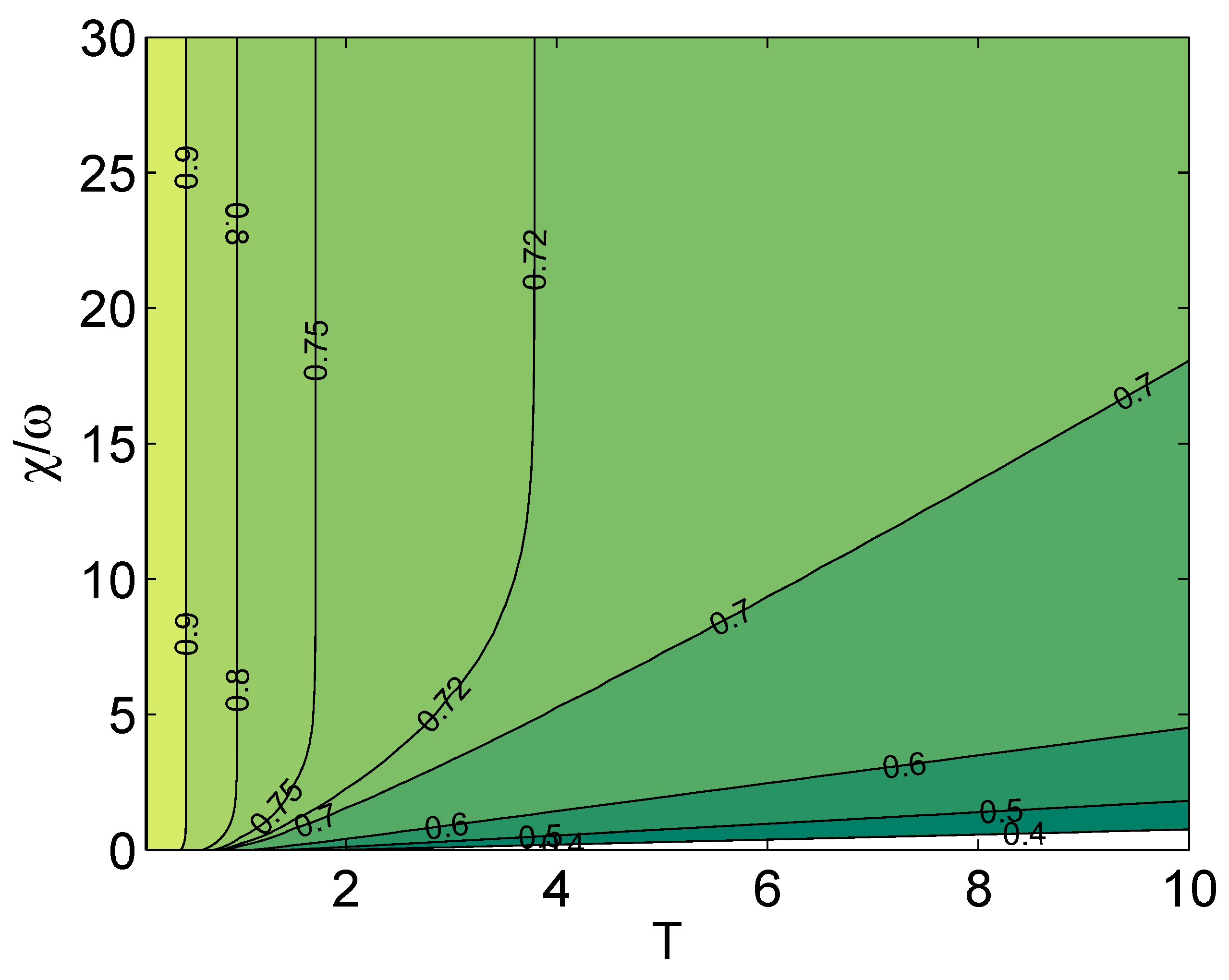
Figure 6 displays FH-order values (Fisher ones) in this plane. The intensity of the color signals the order’s degree. It is clearly seen how order behaves. The planar representation clearly allows one to visualize the regions of order and the regions that lack order.

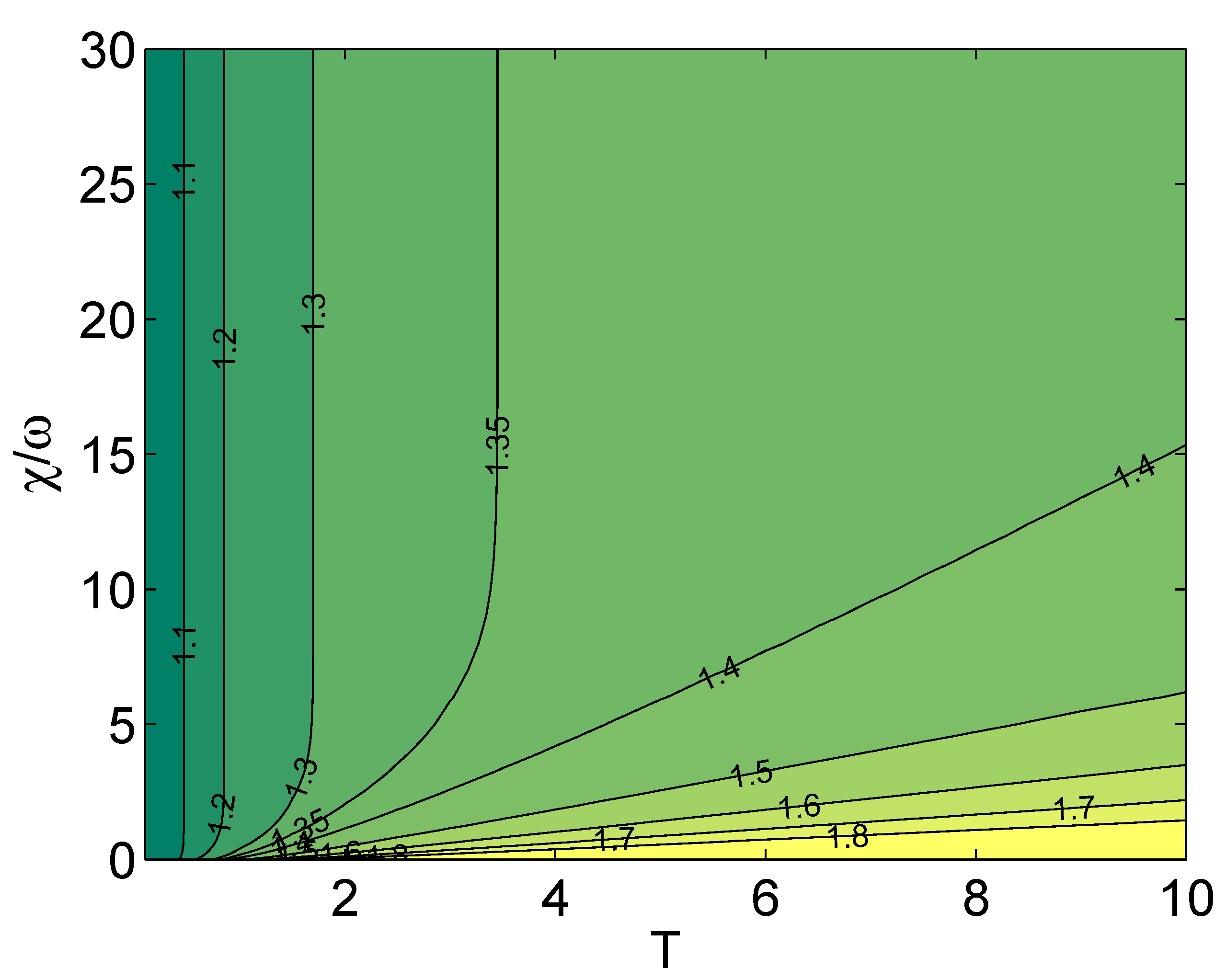
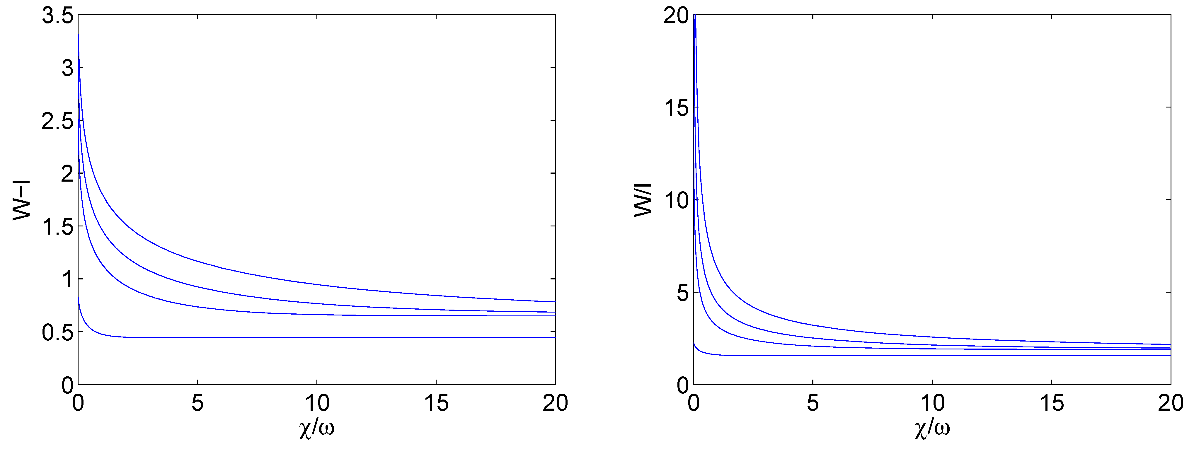
Figure 7 represents the same effects, with reference to disorder and W as the protagonist. Finally, Figure 8 exhibits the convergence between W and the FH-measure to extreme order situations. One of them is that of zero temperature T. The other refers to a very large Kerr effect, $\chi \to \infty$ (because the Kerr interaction tends to align the system along a given spatial direction, thus “ordering” it). To save space, we do not exhibit graphs for Shannon’s entropy, but in the order/disorder question it behaves in similar fashion as the Wehrl’s one.

An important point to be emphasized is that Wehrl’s (Shannon’s) entropy can be regarded as a strict disorder indicator, because it complies with the requirements of Section (2.3). It also coincides with Fisher’s quantifier in the extreme limits of zero temperature and very large Kerr effect. Moreover, if one looks at its behavior in the T vs. χ-plane (of course, T and χ are independent variables), one appreciates the existence of a large region (precisely, that representing minimum degree of disorder, namely, when Lieb’s bound is achieved) in which the quantifier is constant and equal to unity.

Figure 6. Kerr medium. FH-order I in the T vs. χ-plane. The graduation of different colors (east to west, north to south) represents the degree of order.

Figure 6. Kerr medium. FH-order I in the T vs. χ-plane. The graduation of different colors (east to west, north to south) represents the degree of order.

Figure 7. Kerr medium. W in the T vs. χ-plane. The sequence of different colors (east to west, north to south) represents the degree of disorder.

Figure 7. Kerr medium. W in the T vs. χ-plane. The sequence of different colors (east to west, north to south) represents the degree of disorder.

Figure 8. Kerr medium. For T = 1, 5, 10, 20, respectively, from bottom to top, we plot, versus χ/ω, the difference W − I (left) and the ratio W/I (right).

Figure 8. Kerr medium. For T = 1, 5, 10, 20, respectively, from bottom to top, we plot, versus χ/ω, the difference W − I (left) and the ratio W/I (right).

6. Conclusions

We have shown in this paper, with regard to two well-known physical models, that

• the Frieden–Hawkins order-measure behaves in appropriate manner vis-a-vis (i) temperature and (ii) an aligning interaction Hamiltonian.
• The Wehrl or Shannon entropies are as good indicators of disorder as the Fisher’s order measure is of order, given their compliance with the features summarized in Section (2.3). It is intuitively clear that entropy measures disorder. What we are saying here is that, quantitatively, it does it in a way entirely similar to that for order in the FH-case.

These results should encourage further application of the couple (FH-measure-Wehrl entropy) to different scenarios.

References

1. Frieden, B.R.; Hawkins, R.J. Quantifying system order for full and partial coarse graining. Phys. Rev. E 2010, 82. [Google Scholar] [CrossRef]
2. Dimassi, M.; Sjoestrand, J. Spectral Asymptotics in the Semi-Classical Limit; Cambridge University Press: Cambridge, UK, 1999. [Google Scholar]
3. Brack, M.; Bhaduri, R.K. Semiclassical Physics; Addison-Wesley: Reading, MA, USA, 1997. [Google Scholar]
4. Arnheim, R. Entropy and Art: An Essay in Disorder and Order; University of California Press: Berkeley, CA, USA, 1971. [Google Scholar]
5. Darrigol, O. From c-Numbers to q-Numbers; University of California Press: Berkeley, CA, USA, 1992. [Google Scholar]
6. Rosenkrantz, R.D. E.T. Jaynes: Papers on Probability, Statistics and Statistical Physics; D. Reidel: Dordrecht, The Netherlands, 1983. [Google Scholar]
7. M. Gell-Mann, M.; Tsallis, C. Nonextensive Entropy: Interdisciplinary Applications; Oxford University Press: Oxford, UK, 2004. [Google Scholar]
8. Tsallis, C. Introduction to Nonextensive Statistical Mechanics: Approaching a Complex World; Springer: New York, NY, USA, 2009. [Google Scholar]
9. Schrödinger, E. What Is Life? The Physical Aspect of the Living Cell and Mind and Matter; Cambridge University Press: New York, NY, USA, 1967. [Google Scholar]
10. Frieden, B.R.; Plastino, A.; Plastino, A.R. Fisher order measure and Petri’s universe. Phys. A 2012, 391, 2300–2305. [Google Scholar] [CrossRef]
11. Frieden, B.R.; Gatenby, R.A. Order in a multidimensional system. Phys. Rev. E 2011, 84. [Google Scholar] [CrossRef]
12. Frieden, B.R.; Plastino, A.; Plastino, A.R. Effect upon universal order of Hubble expansion. Phys. A 2011, 391, 410–413. [Google Scholar] [CrossRef]
13. Frieden, B.R. Science from Fisher Information, 2 ed.; Cambridge University Press: Cambridge, UK, 2004. [Google Scholar]
14. Kolmogorov, A.N. Three approaches to the quantitative definition of information. Problems Inform. Transmission 1965, 1, 1–7. [Google Scholar] [CrossRef]
15. Chaitin, G.J. On the simplicity and speed of programs for computing infinite sets of natural numbers. J. ACM 1969, 16, 407–422. [Google Scholar] [CrossRef]
16. Bradley, C.C.; Sackett, C.A.; Hulet, R.G. Bose-Einstein condensation of lithium: Observation of limited condensate number. Phys. Rev. Lett. 1997, 78, 985–989. [Google Scholar] [CrossRef]
17. Anderson, M.H.; Ensher, J.R.; Matthews, M.R.; Wieman, C.E.; Cornell, E.A. Observation of Bose-Einstein condensation in a dilute atomic vapor. Science, 1995, 269, 198–201. [Google Scholar] [CrossRef] [PubMed]
18. Davis, K.B.; Davis, K.B.; Mewes, M.O.; Andrews, M.R.; van Druten, N.J.; Durfee, D.S.; Kurn, D.M.; Ketterle, W. Bose-Einstein condensation in a gas of sodium atoms. Phys. Rev. Lett. 1995, 75, 3969–3973. [Google Scholar] [CrossRef] [PubMed]
19. Wigner, E.P. On the quantum correction for thermodynamic equilibrium. Phys. Rev. 1932, 40, 749–759. [Google Scholar] [CrossRef]
20. Weyl, H. Quantenmechanik und gruppentheorie. Z. Phys. 1927, 46, 1–46. [Google Scholar] [CrossRef]
21. Moyal, J.E. Stochastic processes and statistical physics. J. Roy. Stat. Soc. B 1949, 11, 150–210. [Google Scholar]
22. Zachos, C.; Fairlie, D.; Curtright, T. Quantum Mechanics in Phase Space; World Scientific: Singapore, 2005. [Google Scholar]
23. Lee, H.W. Theory and application of the quantum phase-space distribution functions. Phys. Rep. 1995, 259, 147–211. [Google Scholar] [CrossRef]
24. Wlodarz, J.J. Entropy and Wigner distribution functions revisited. Int. J. Theor. Phys. 2003, 42, 1075–1084. [Google Scholar] [CrossRef]
25. Krivine, H.; Casas, M.; Martorell, J. Semiclassical expansions for confined n fermion systems. Ann. Phys. (NY) 1990, 200, 304–344. [Google Scholar] [CrossRef]
26. Ozorio de Almeida, A.M. The Weyl representation in classical and quantum mechanics. Phys. Rep. 1998, 295, 265–342. [Google Scholar] [CrossRef]
27. Husimi, K. Some formal properties of the density matrix. Proc. Phys. Math. Soc. Jpn. 1940, 22, 264–283. [Google Scholar]
28. Mizrahi, S.S. Quantum mechanics in the Gaussian wave-packet phase space representation. Phys. A 1984, 127, 241–264. [Google Scholar] [CrossRef]
29. Pennini, F.; Ferri, G.L.; Plastino, A. Fisher information and semiclassical treatments. Entropy 2009, 11, 972–992. [Google Scholar] [CrossRef]
30. O’ Connell, R.F.; Wigner, E.P. Some properties of a non-negative quantum-mechanical distribution function. Phys. Lett. A 1981, 85, 121–126. [Google Scholar] [CrossRef]
31. Mizrahi, S.S. Quantum mechanics in the Gaussian wave-packet phase space representation II: Dynamics. Phys. A 1986, 135, 237–250. [Google Scholar] [CrossRef]
32. Mizrahi, S.S. Quantum mechanics in the gaussian wave-packet phase space representation III: From phase space probability functions to wave-functions. Phys. A 1988, 150, 541–554. [Google Scholar] [CrossRef]
33. Anderson, A.; Halliwell, J.J. Information-theoretic measure of uncertainty due to quantum and thermal fluctuations. Phys. Rev. D 1993, 48, 2753–2765. [Google Scholar] [CrossRef]
34. Zurek, W.H. Sub-Planck structure in phase space and its relevance for quantum decoherence. Nature 2001, 412, 712–717. [Google Scholar] [CrossRef] [PubMed]
35. Karkuszewski, Z.P.; Jarzynski, C.; Zurek, W.H. Quantum chaotic environments, the butterfly effect, and decoherence. Phys. Rev. Lett. 2002, 89. [Google Scholar] [CrossRef]
36. Wisniacki, D.A. Short-time decay of the Loschmidt echo. Phys. Rev. E 2003, 67. [Google Scholar] [CrossRef]
37. Rivas, A.M.F.; Vergini, E.G.; Wisniacki, D.A. Smoothed Wigner functions: A tool to resolve semiclassical structures. Eur. Phys. J. D 2005, 32, 355–359. [Google Scholar] [CrossRef]
38. Manfredi, G.; Feix, M.R. Entropy and Wigner functions. Phys. Rev. E 2000, 62, 4665–4674. [Google Scholar] [CrossRef]
39. Rivas, A.M.F.; Ozorio de Almeida, A.M. Hyperbolic scar patterns in phase space. Nonlinearity 2002, 15, 681–693. [Google Scholar] [CrossRef]
40. Wehrl, A. On the relation between classical and quantum entropy. Rep. Math. Phys. 1979, 16, 353–358. [Google Scholar] [CrossRef]
41. Glauber, R.J. Coherent and incoherent states of the radiation field. Phys. Rev. 1963, 131, 2766–2788. [Google Scholar] [CrossRef]
42. Klauder, J.R.; Skagerstam, B.S. Coherent States; World Scientific: Singapore, 1985. [Google Scholar]
43. Pennini, F.; Plastino, A. Thermal effects in quantum phase-space distributions. Phys. Lett. A 2010, 374, 1927–1932. [Google Scholar] [CrossRef]
44. Olivares, F.; Pennini, F.; Plastino, A. Phase space distributions from variation of information measures. Phys. A 2010, 389, 2218–2226. [Google Scholar] [CrossRef]
45. Pennini, F.; Plastino, A.; Ferri, G.L. Statistical, noise-related non-classicality’s indicator. Central Eur. J. Phys. 2009, 7, 624–629. [Google Scholar] [CrossRef]
46. Pennini, F.; Plastino, A.; Ferri, G.L.; Olivares, F.; Casas, M. Information, Deformed, κ-Wehrl entropies and semiclassical delocalization. Entropy 2009, 11, 32–41. [Google Scholar] [CrossRef] [Green Version]
47. Pennini, F.; Plastino, A. Smoothed Wigner distributions, decoherence, and the temperature dependence of the classical-quantical frontier. Eur. Phys. J. D. 2011, 61, 241–247. [Google Scholar] [CrossRef]
48. Haus, H. Waves and Fields Optoelectronics; Prentice Hall: New York, NY, USA, 1984. [Google Scholar]
49. Wilson-Gordon, A.D.; V. Buz̆ec, V.; Knight, P.L. Statistical and phase properties of displaced Kerr states. Phys. Rev. A 1991, 44, 7647–7656. [Google Scholar] [CrossRef] [PubMed]
50. Olivares, F.; Pennini, F.; Ferri, G.L.; Plastino, A. Note on semiclassical uncertainty relations. Braz. J. Phys. 2009, 39, 503–506. [Google Scholar] [CrossRef]