Article

Expectation Values and Variance Based on Lp-Norms

Southwest Research Institute, San Antonio, TX-78238, USA
Entropy 2012, 14(12), 2375-2396; https://doi.org/10.3390/e14122375
Submission received: 4 August 2012 / Revised: 13 November 2012 / Accepted: 14 November 2012 / Published: 26 November 2012

Abstract

:
This analysis introduces a generalization of the basic statistical concepts of expectation values and variance for non-Euclidean metrics induced by L p -norms. The non-Euclidean L p means are defined by exploiting the fundamental property of minimizing the L p deviations that compose the L p variance. These L p expectation values embody a generic formal scheme of means characterization. Having the p-norm as a free parameter, both the L p -normed expectation values and their variance are flexible to analyze new phenomena that cannot be described under the notions of classical statistics based on Euclidean norms. The new statistical approach provides insights into regression theory and Statistical Physics. Several illuminating examples are examined.

1. Introduction

2500 years after the Pythagorean discipline and the “self-imposed" intense study on the arithmetic, geometric and harmonic means, the power-means of the elements { y i } i = 1 N , y i D y , i = 1 , , N , given by M p ( { y i } i = 1 N ) = ( i = 1 N y i p / N ) 1 / p , were introduced [1] as suitable generalization of the former Pythagorean ones, for p = 1 , 0 , - 1 , respectively. An even more general characterization, preceded of the power-means, concerns the Kolmogorov–Nagumo means [2,3], also known as φ -means, which are expressed in terms of a strictly monotonic function φ , as M φ ( { y i } i N ) = φ - 1 [ i = 1 N φ ( y i ) / N ] .
Hardy et al. [4] showed that the φ -means are characterized by various fundamental properties of the ordinary arithmetic means. Later, Ben-Tal [5] showed that the φ -means are indeed ordinary arithmetic means defined on linear spaces with suitably chosen operations of addition and multiplication. The latter justifies the φ -means alternative names of “quasilinear" [4] or “quasiarithmetic” [6]. The series { y i } i = 1 N can be rearranged, according to the y-values of its elements, to the set { y k } k = 1 W , where each value y k has possibility p k = Δ N k N , with Δ N k being the number of elements { y i } i = 1 N that follow the equality y i = y k (for examples, see [7]). However, the probability distribution { p k } k = 1 W can be constructed directly in association with { y k } k = 1 W , and without the necessity of the series { y i } i = 1 N . Then, the relation p k = p k ( { y k } k = 1 W ) , k = 1 , , W can be derived. These weighted φ -means were introduced by [8], and expressed in terms of the probability distribution { p k } k = 1 W , namely, M φ ( { y k } k = 1 W ) = φ - 1 [ k = 1 W p k φ ( y k ) ] , giving advance to the axiomatic theory of information functions [9].
The φ -means are found to have useful applications in a variety of topics, namely, in statistics [10], in decision theory [11], in signal processing [12], in thermostatistics [13,14], etc. Within the framework of signal processing, [12] succeeded in specifying classes of signals associated with the quasiarithmetic mean of two variables. However, the main efforts to use the φ -means to this topic, are typically addressed in signal denoising processes. For example, by applying the power-means, the moving average shifts towards small signal values for small p and emphasizes large signal values for large p, thus highlighting the fluctuations of the preferred scaling. As soon as the nonlinear function φ is appropriately chosen, φ -means-based filters can efficiently reduce noise at a preferred scale of signal values. Another significant nonlinear filtering scheme, having interesting properties in signal denoising, is based on the moving median, instead of the moving φ -means technique [15,16]. Lately, the median value found to play a key-point role in signal processing optimization and block entropy analysis [7,17]. The median is based on the non-Euclidean norm L 1 (Taxicab norm), and thus, it does not embody the characterization of φ -means, which are in their basis Euclidean, i.e., they are induced by the Euclidean norm L 2 [18].
In [7] a novel generalized characterization of means was introduced, namely, the non-Euclidean means, based on metrics induced by L p norms, wherein the median is included as special case for p = 1 ( L 1 ), while the non-Euclidean φ -means can also be defined. (See also the work of [19], where the general clustering approaches is investigated using, among others, similar well-defined means based on non-Euclidean optimization.) In this way, the L p expectation value of a given energy spectrum { ε k } k = 1 W is defined, representing the non-Euclidean adaptation of internal energy U p . (This issue is mentioned in Section 3.1; it can be further examined in the framework of non-Euclidean-normed Statistical Mechanics.)
The Euclidean norm L 2 is also known as “Pythagorean" norm. Hereafter, we prefer referring to the non-Pythagorean norms as non-Euclidean, inheriting the same characterization to Statistics. One may adopt the more explicit characterizations of “non-Euclidean-normed" statistics, for avoiding any confusion with the non-Euclidean metric of the (Euclidean-normed) Riemannian geometry.
The paper is organized as follows. In Section 2, the L p means are defined, resulting from the minimization of the respective L p deviations. Similarly, the more generic Φ-normed φ -means are also defined. The general scheme of means characterization, wherein the L p means are embodied, is given. In Section 3, the concept of L p -expectation values is thoroughly studied. The L p means are expressed in terms of the L ^ p operator, which helps to automatically retrieve the non-Euclidean representation of a formulation from its respective Euclidean one. The non-Euclidean expectation and variance operators are accordingly deduced. Several examples of Statistical Mechanics are examined: gas in thermal equilibrium, space plasmas out of thermal equilibrium, and multi-dimensional quantum harmonic oscillator at thermal equilibrium. Section 4 introduces the L p variance; its expression is justified and examined in detail. In Section 5, some further analytical and numerical examples are examined. It is shown that in the case of symmetric distributions of data, the whole set of L p means degenerate to one single value, while for asymmetric ones, spectrum-like range of L p means is generated. In addition, we deal with numerical data of the magnitude of Earth’s total magnetic field. Finally, Section 6 draws the conclusions.

2. The Generalized Formal Scheme of Means Characterization

2.1. The Means Characterization Based on Optimization Methods

The non-Euclidean means μ p , based on L p norms, are defined as follows
k = 1 W p k | y k - μ p | p - 1 s i g n ( y k - μ p ) = 0
where the median μ 1 and the arithmetic mean μ 2 follow as special cases for the Taxicab L 1 and Euclidean L 2 , respectively. Both the median μ 1 and arithmetic μ 2 means can be implicitly written in the form of Equation (1) as k = 1 W p k s i g n ( y k - μ 1 ) = 0 and k = 1 W p k | y k - μ 2 | s i g n ( y k - μ 2 ) = 0 ( μ 2 = k = 1 W p k y k ), respectively. These forms can be thought as the result of the corresponding optimizations of the Total Absolute Deviations T A D ( { y k } k = 1 W ; α ) = k = 1 W p k | y k - α | (also called Total Boundary Area - TBA), and the Total Square Deviations T S D ( { y k } k = 1 W ; α ) 2 = k = 1 W p k | y k - α | 2 , for describing the optimal values α * = μ 1 and α * = μ 2 , respectively [7,18,20]. Similarly, the L p mean μ p emerges from minimizing the Total p-Deviations, i.e.,
T D p ( { y k } k = 1 W ; α ; p ) p = k = 1 W p k | y k - α | p
The optimization leads to (i) the normal Equation (1), from which the optimal parameter α * = μ p can be derived as an implicit expression of p, (ii) the total deviations minimum value T D p , M i n ( { y k } k = 1 W ; p ) p = k = 1 W p k | y k - α * | p , which is the pth absolute moment at the L p mean α * = μ p . Therefore, the Euclidean mean μ 2 , known as the one minimizing the (Euclidean) variance, is generalized to the L p mean μ p , which is the one minimizing the L p variance, a quantity proportional to T D p ( { y k } k = 1 W ; α ; p ) p (Section 3.1, Section 4).
The generalized L p φ -means μ ( φ , p ) can be defined given the strictly monotonic function φ : y k z k = φ ( y k ) , k = 1 , , W , i.e.,
k = 1 W p k | φ ( y k ) - φ ( μ ( φ , p ) ) | p - 1 s i g n φ ( y k ) - φ ( μ ( φ , p ) ) = 0
which is the normal equation derived from the Total ( φ , p ) -Deviations,
T D ( φ , p ) ( { y k } k = 1 W ; α ; p ) p = k = 1 W p k | φ ( y k ) - φ ( α ) | p
Thereafter, we arrive at the classical φ -means μ ( φ , p = 2 ) = M φ by considering the Euclidean norm. Even further, by considering an arbitrary functional norm Φ : u Φ ( | u | ) ( Φ ( 0 ) = 0 ), the Total ( φ , Φ ) -Deviations are formulated
Φ T D ( φ , Φ ) ( { y k } k = 1 W ; α ) = k = 1 W p k Φ | φ ( y k ) - φ ( α ) |
leading to the normal equation
k = 1 W p k Φ ´ | φ ( y k ) - φ ( μ ( φ , Φ ) ) | s i g n φ ( y k ) - φ ( μ ( φ , Φ ) ) = 0
from which we obtain the Φ-normed φ -means μ ( φ , Φ ) . It is noted that the solution of Equation (5) is generally called M-estimator, a broad class of estimators, which are obtained by minimizing the sums of functions of data. An M-estimator can be defined to be a zero of an estimating function that often is the derivative of another statistical function. When this differentiation is possible, leading to Equation (6), the M-estimator is said to be of ψ-type. (For more on M-estimators theory, see [21,22].)

2.2. Formal Scheme of Means Characterization

The characterization of means based on optimization methods has already been found useful, providing insights into the optimization theory and its applications (e.g., see [7]). The most important application involves reestablishing the concept of expectation values. However, we have to be certain that the optimization characterization of means, as described in Section 2.1, can embody the general scheme of means characterization.
Aczél [23] suggested an axiomatic characterization of means, settled by five fundamental properties of the ordinary arithmetic means, and succeeded to reproduce the φ -means. In particular, any univalued, bivariable function M ( y 1 , y 2 ) , y 1 , y 2 D y constitutes a general mean of y 1 , y 2 , if the following preconditions are fulfilled: (i) Continuity; (ii) Strict monotonicity: if y 1 < y 1 ´ (>), then M ( y 1 , y 2 ) < M ( y 1 ´ , y 2 ) (>), and the same holds for y 2 < y 2 ´ ; (iii) Bisymmetry: M ( M ( y 1 , y 2 ) , M ( y 3 , y 4 ) ) = M ( M ( y 1 , y 3 ) , M ( y 2 , y 4 ) ) ; (iv) Reflexivity: M ( y , y ) = y ; (v) Symmetry: M ( y 1 , y 2 ) = M ( y 2 , y 1 ) . Aczél also proved [24] that, if and only if the (i)–(iv) preconditions are fulfilled, then M ( y 1 , y 2 ) = φ - 1 [ λ φ ( y 1 ) + ( 1 - λ ) φ ( y 2 ) ] , y 1 , y 2 D y , 0 < λ < 1 , and φ : strictly monotonic function. For λ = 1 / 2 , (v) is also fulfilled, hence, M ( y 1 , y 2 ) coincides with the φ -mean of y 1 , y 2 , i.e., M ( y 1 , y 2 ) = M φ ( y 1 , y 2 ) .
Aczél also pointed [23] that the “internness” property, i.e., M i n ( y 1 , y 2 ) M ( y 1 , y 2 ) M a x ( y 1 , y 2 ) , follows from preconditions (i), (ii), (iv). However, it is evident that the internness, together with the continuity (i), leads to the reflexivity (iv). This remark implies that we can settle the internness as precondition, instead of the strict monotonicity and reflexivity. (Besides, the median does not follow strict monotonicity, while it follows the internness. In addition, internness ensures that the mean shall preserve the units of y-values under units-transformations.) Then, turning aside of preconditions (ii) and (iii) that entail the Euclidean character of φ -means, an alternative characterization of means can be given by the univalued, N-multivariable function M ( { y i } i = 1 N ) , fulfilling the three preconditions: (i) Continuity; (ii) Internness: M i n ( { y i } i = 1 N ) M ( { y i } i = 1 N ) M a x ( { y i } i = 1 N ) ; (iii) Symmetry: For y i y j i , i = 1 , , N : { y i } i = 1 N = { y j i } i = 1 N , then M ( { y i } i = 1 N ) = M ( { y j i } i = 1 N ) . (This characterization considered also by [25] for N = 2 .)
It can be easily verified that the non-Euclidean, Φ-normed, φ -means μ ( Φ , φ ) obey to the above characterization. Throughout, we deal with the L p means μ p . The uniqueness of μ p means can be provided for any p 1 . (The restriction p 1 is required for the triangle inequality of the norm’s definition to hold.) In particular, the non-zero derivative
p μ p = ( p - 1 ) k = 1 W p k | y k - μ p | p - 2 k = 1 W p k | y k - μ p | p - 1 s i g n ( y k - μ p ) ln ( | y k - μ p | ) , p > 1
and the fact that the derivatives of any order of μ p ( p ) , inductively, are analytically expressed in terms of the (univalued) Euclidean mean μ p ( p ) | p = 2 = μ 2 , can ensure for the uniqueness of μ p , for a given p > 1 (for p = 1 , see [7]). Note that for the specific case where k = k : y k = μ p , then for p < 2 , Equation (7) gives p / μ p ( p - 1 ) / [ ( y k - μ p ) ln ( | y k - μ p | ) ] , i.e., μ p / p 0 .

3. The Concept of L p -Expectation Values

3.1. The Non-Euclidean Norm Operator L ^ p

The non-Euclidean L p -expectation value y p is implicitly given by
k = 1 W p k | y k - y p | p - 1 s i g n ( y k - y p ) = 0
and it is apparent that the most of the fundamental properties of the Euclidean expectation value are not inherited by the non-Euclidean expectation values. In particular, we distinguish among others, the following two Euclidean properties: (i) y 2 = k = 1 W p k y k (by definition), and (ii) β y 2 = k = 1 W p k β y k , for a given parameter β, for which p k = p k ( { y k } k = 1 W ; β ) , k = 1 , , W , and y p = y p ( { y k } k = 1 W ; β ) . Now, we examine whether the above two properties can be fulfilled even for the case of non-Euclidean L p -expectation value y p , and a suitably transformed data set { y k ( p ) } k = 1 W , namely, (i) y p = k = 1 W p k y k ( p ) , and (ii) β y p = k = 1 W p k β y k ( p ) . Indeed, this is true for the specific transformation L ^ p : y k y k ( p ) L ^ p ( y k ) , k = 1 , , W , where L ^ p denotes the non-Euclidean norm operator, i.e.,
L ^ p ( y k ) = | y k - y p | p - 1 s i g n ( y k - y p ) ( p - 1 ) ϕ p + y p
where ϕ p k = 1 W p k | y k - y p | p - 2 . Finally, L ^ p exhibits the following properties:
(i)
The non-Euclidean mean of { y k } k = 1 W is the Euclidean mean of { L ^ p ( y k ) } k = 1 W
y p = L ^ p ( y ) 2 = k = 1 W p k L ^ p ( y k )
(ii)
Zero-mean of { β L ^ p ( y k ) } k = 1 W ,
0 = k = 1 W p k β L ^ p ( y k ) , or , β y p = k = 1 W p k β L ^ p ( y k )
(iii)
Norm-derivative (Equation (7)):
y p p = k = 1 W p k p L ^ p ( y k ) + k = 1 W p k L ^ p ( y k - y p ) ln | y k - y p |
y p p = k = 1 W p k L ^ p ( y k - y p ) ln | y k - y p | , if p k p = 0
(iv)
In the Euclidean case, L ^ p degenerates to the identity operator L ^ p = 2 = 1 ^ .
(v)
Linear operations: L ^ p ( λ y k + c ) = λ L ^ p ( y k ) + c , λ , c .
Hence, y - y p p = L ^ p ( y - y p ) 2 = 0 , which reads Equation (8).
(vi)
Non-additivity of L ^ p : L ^ p ( y k + z k ) L ^ p ( y k ) + L ^ p ( z k ) .
(vii)
Inverse of non-Euclidean norm operator, L ^ p - 1 , L ^ p - 1 L ^ p = L ^ p L ^ p - 1 = 1 ^ ,
L ^ p - 1 ( y k ) = | y k - y p | 1 p - 1 s i g n ( y k - y p ) [ ( p - 1 ) ϕ p ] 1 1 - p + y p
As we mentioned in property (v), Equation (8) can be rewritten in the form L ^ p ( y - y p ) 2 = 0 , or C · k = 1 W p k | y k - y p | p - 1 s i g n ( y k - y p ) = 0 , with C = 1 ( p - 1 ) ϕ p . Obviously, this leads to Equation (8), for any value of the scalar C 0 . However, property (ii) is fulfilled if and only if C has the specific expression C = 1 ( p - 1 ) ϕ p (see further below). Property (ii) is important when we incorporate the non-Euclidean-normed Statistics in Statistical Mechanics: (a) The Canonical probability distribution can be automatically derived and explicitly expressed. (If the scalar C were expressed by any other formulation, after the extremization of entropy in the Canonical Ensemble, we would not be able to solve in terms of the probability, namely, to express explicitly the probability in terms of the energy.) (b) The basic relation that connects Statistical Mechanics with Thermodynamics has to remain the same with the classical case. Namely, the classical relation between the derivative of the partition function Z p and the mean energy (internal energy) U p has to remain invariant, independently of the p-norm. In other words, if L ^ p ( ε k ) = C | ε k - U p | p - 1 s i g n ( ε k - U p ) + U p , then the specific expression of the scalar C = 1 ( p - 1 ) ϕ p , yields the following scheme:
U p = - ln Z p β C = 1 ( p - 1 ) ϕ p k = 1 W p k β L ^ p ( ε k ) = 0
where the non-Euclidean L p expectation value of energy states { ε k } k = 1 W yields the internal energy ε p = U p , while the L p Canonical partition function Z p (in Boltzmann–Gibbs Statistical Mechanics) is given by Z p ( { ε k } k = 1 W ) = k = 1 W exp [ - β L ^ p ( ε k ) ] . Indeed, we have
- ln Z p β = ( C β ) β k = 1 W p k | ε k - U p | p - 1 s i g n ( ε k - U p ) + U p + 1 - C ( p - 1 ) k = 1 W p k | ε k - U p | p - 2 β U p β = U p + 1 - C ( p - 1 ) ϕ p β U p β ,
which equals U p , if and only if C = 1 ( p - 1 ) ϕ p . On the other hand, we have
k = 1 W p k β L ^ p ( ε k ) = C β k = 1 W p k | ε k - U p | p - 1 s i g n ( ε k - U p ) + U p β × 1 - C ( p - 1 ) k = 1 W p k | ε k - U p | p - 2 = U p β 1 - C ( p - 1 ) ϕ p ,
which equals zero, leading to Equation (11), if and only if C = 1 ( p - 1 ) ϕ p .
Given the set of states { y k } k = 1 W of a physical quantity, which are included in the Euclidean representation of a formulation F [ { y k } k = 1 W ] , the respective non-Euclidean representation can be often retrieved automatically by replacing y k with L ^ p ( y k ) , k = 1 , , W , i.e., F p [ { y k } k = 1 W ] = F [ { L ^ p ( y k ) } k = 1 W ] . As an example, the L p Canonical partition function in Boltzmann–Gibbs Statistical Mechanics is given by
Z ( { ε k } k = 1 W ) k = 1 W exp ( - β ε k ) Z p ( { ε k } k = 1 W ) = Z ( { L ^ p ( ε k ) } k = 1 W ) ,
where { ε k } k = 1 W is a discrete energy spectrum.
Consequently, according to the above considerations, the non-Euclidean L p -expectation estimator E ^ p , acting on a random variable Y, is given by
E ^ p ( Y ) = E ^ 2 L ^ p ( Y )
where E ^ 2 ( E ^ ) is the classical (Euclidean) expectation estimator.
On the other hand, the non-Euclidean L p -variance estimator σ 2 ^ p has to result to the Total p-Deviations of Equation (2), or at least, to be proportional to that, such that its minimization leads to Equation (1). This can be achieved by setting,
σ 2 ^ p = E 2 ^ ( Y - Y p ) L ^ p ( Y - Y p )
(Section 4 revisits the concept of non-Euclidean L p -variance, providing a convincing and consistent justification of Equation (17).) Finally, given a set of random variables { Y i } i = 1 n , the non-Euclidean covariance estimator ( σ 2 ^ p ) i j is given by
( σ 2 ^ p ) i j = E ^ 2 ( Y i - Y i p ) L ^ p ( Y j - Y j p )

3.2. The Non-Euclidean L p -Mean Estimator and Its Expectation Value

Two basic theorems of the ordinary expectation values are inherited to the non-Euclidean ones: (1) The L p -expectation value of the L p -mean estimator μ ^ p , N ( { y j } j = 1 N ; p ) is equal to the L p -expectation value μ p of any of the independent and identically distributed random variables { y j } j = 1 N . (2) The L p -mean estimator μ ^ p , N converges to its L p -expectation value, μ ^ p , N p = E ^ p ( μ ^ p , N ) = μ p , as N .
Given the sampling { y i } i = 1 N , the non-Euclidean, L p -mean estimator μ ^ p , N = μ ^ p , N ( { y j } j = 1 N ; p ) is implicitly expressed by
i = 1 N | y i - μ ^ p , N ( { y j } j = 1 N ; p ) | p - 1 s i g n [ y i - μ ^ p , N ( { y j } j = 1 N ; p ) ] = 0
Then, the non-Euclidean L p -expectation value of μ ^ p , N , namely, μ ^ p , N p E ^ p ( μ ^ p , N ( { y j } j = 1 N ; p ) ) , is implicitly given by
{ y j D y } j = 1 N μ ^ p , N ( { y j } j = 1 N ; p ) - μ ^ p , N p p - 1 s i g n [ μ ^ p , N ( { y j } j = 1 N ; p ) - μ ^ p , N p ] × L ( { y j } j = 1 N ) d y 1 d y N = 0
where L ( { y j } j = 1 N ) is the normalized joint probability density, so that
{ y j D y } j = 1 N L ( { y j } j = 1 N ) d y 1 d y N = 1
Consider the sampling { y i } i = 1 N , y i D y R , i = 1 , , N , of the symmetrically distributed random variables { Y i } i = 1 N . Namely, the joint distribution density has the property L ( { y j } j = 1 N ) = L ( y 1 . . . y k . . . y i . . . y N ) = L ( y 1 . . . y i . . . y k . . . y N ) , i , k ( i ) = 1 , , N .
Lemma 1
The symmetrically distributed random variables { Y i } i = 1 N are characterized by the same non-Euclidean L p -expectation value, namely, Y i p = E ^ p ( Y i ) = μ p R , i = 1 , , N , implicitly given by
{ y j D y } j = 1 N y i - μ p p - 1 s i g n y i - μ p L ( { y j } j = 1 N ) d y 1 d y N =
= y i D y y i - μ p p - 1 s i g n y i - μ p L y ( y i ) d y i = 0
where L y i ( u ) L y ( u ) , i = 1 , , N , is the marginal distribution density, which is identical for all the random variables { Y i } i = 1 N .
Lemma 2
Let the auxiliary functionals { G i } i = 1 N , with G i = G i ( { y j } j = 1 N ; p ) y i - μ ^ p , N ( { y j } j = 1 N ; p ) , i = 1 , , N . Then, their L p -expectation values are zero, namely, G i p = E ^ p ( G i ) = 0 , i = 1 , , N .
Theorem 1
Consider the sampling { y i } i = 1 N , y i D y R , i = 1 , , N , of the symmetrically distributed random variables { Y i } i = 1 N . According to Lemma 1, the random variables are characterized by the same non-Euclidean L p -expectation value, namely, Y i p = E ^ p ( Y i ) = μ p R , i = 1 , , N , which is implicitly expressed by Equation (22). Then, the L p -expectation value of the L p -mean estimator μ ^ p , N ( { y j } j = 1 N ; p ) is equal to μ p , i.e., μ ^ p , N p = E ^ p ( μ ^ p , N ( { y j } j = 1 N ; p ) ) = μ p :
{ y j D y } j = 1 N | μ ^ p , N ( { y j } j = 1 N ; p ) - μ p | p - 1 s i g n [ μ ^ p , N ( { y j } j = 1 N ; p ) - μ p ] × L ( { y j } j = 1 N ) d y 1 d y N = 0
Theorem 2
Consider the sampling { y i } i = 1 N , y i D y R , i = 1 , , N , of the independent and identically distributed random variables { Y i } i = 1 N . The L p -mean estimator μ ^ p , N ( { y j } j = 1 N ; p ) converges to its L p -expectation value, μ ^ p , N p = E ^ p [ μ ^ p , N ( { y j } j = 1 N ; p ) ] = μ p , as N , namely, lim N μ ^ p , N = μ ^ p , N p = μ p . Remark: The independent and identically distributed random variables are also symmetrically distributed. Then, from Theorem 1 we have μ ^ p , N p = E ^ p [ μ ^ p , N ( { y j } j = 1 N ; p ) ] = Y i p = E ^ p ( Y i ) = μ p . The L p -expectation value Y i p = μ p is calculated given the marginal distribution density L y ( y i ) , i = 1 , , N . However, the expression of this distribution is in the generic case unknown, and thus, we estimate μ p by means of μ ^ p , N for N > > 1 .

3.3. Examples

In the following three examples from Statistical Mechanics, we examine the systems of (1) gas in thermal equilibrium, (2) space plasmas out of thermal equilibrium, and (3) multi-dimensional quantum harmonic oscillator at thermal equilibrium. The non-Euclidean-normed internal energy U p is derived by utilizing the classical Euclidean probability distribution of Canonical Ensemble.

3.3.1. Gas at Thermal Equilibrium

For the continuous energy spectrum ε [ 0 , ) with distribution p ( ε ) and degeneracy g ( ε ) , the L p internal energy ε p is given by
0 p ( ε ) g ( ε ) | ε - ε p | p - 1 s i g n ( ε - ε p ) = 0
At classical thermal equilibrium, the energy distribution is given by the Boltzmann–Gibbs distribution p ( ε ) e - ε k B T . The degeneracy is g ( ε ) ε f 2 - 1 , where f denotes the degrees of freedom. Hence, the internal energy, ε p / ( k B T ) , is implicitly expressed in terms of p, f, as follows
0 e - x x f 2 - 1 | x - ε p k B T | p - 1 s i g n x - ε p k B T = 0
where we set x ε / ( k B T ) . In the Euclidean case, the internal energy is ε 2 = ( f / 2 ) k B T . In the non-Euclidean case, this is written as ε p = ( f p / 2 ) k B T , where f p represents the reflected degrees of freedom; for sufficiently high number of degrees we find f p f + 0 . 66 · ( p - 2 ) .

3.3.2. Plasma Out of Thermal Equilibrium

Classical systems are said to be in thermal equilibrium – the concept that any flow of heat (thermal conduction, thermal radiation) is in balance. However, thermal equilibrium is not the only possible state that is stationary (i.e., the phase space distribution does not explicitly depend on time). For example, space plasmas are systems residing in stationary states but out of thermal equilibrium. For these systems, the energy distribution is well-described by the empirical kappa distribution (see [26] and references therein). Moreover, the kappa distribution was shown to be connected [26] with the solid background of non-extensive Statistical Mechanics [27], and represents the probability distribution that maximizes entropy in the Canonical Ensemble. The kappa distribution is the generalization of the classical Boltzmann–Gibbs exponential distribution that describes systems only at thermal equilibrium. The temperature and the kappa index that govern these distributions are the two independent controlling parameters of non-equilibrium systems. The invariant form of the kappa distribution, in which the temperature T, the kappa index κ 0 and the total degrees of freedom f are all independent variables [28], is given by
P ( ε ; T ; κ 0 ; f ) 1 + 1 κ 0 · ε k B T - κ 0 - 1 - f 2
where the kappa index ( κ 0 > 0 ) determines a measure of how far the system is from the thermal equilibrium [29]. The kappa distribution recovers the Boltzmannian exponential distribution for κ 0 , which is the value of the kappa index characterizing thermal equilibrium. The smallest possible value of the kappa index is κ 0 0 , and determines the furthest stationary state from thermal equilibrium [30].
In Figure 1 the kappa distribution P ( ε ; T ; κ 0 ; f ) g ( ε ) × ( k B T ) is depicted in terms of ε / ( k B T ) for κ 0 = 0 . 01 , 0 . 1 , 1 , 10 . The internal energy ε p is given by
0 1 + x κ 0 - κ 0 - 1 - f 2 x f 2 - 1 | x - ε p k B T | p - 1 s i g n x - ε p k B T = 0
(Again, we set x ε / ( k B T ) and the degeneracy is g ( ε ) ε f 2 - 1 .) In Figure 2a we depict the internal energy, ε p / ( 1 / 2 k B T ) with respect to the degrees of freedom f, for p = 1 . 5 , 2 , 2 . 5 and for kappa indices κ 0 = 1 . 5 and κ 0 = 100 (this practically equals the Boltzmannian exponential distribution at thermal equilibrium). Figure 2b plots the internal energy over the degrees of freedom, ε p / ( f / 2 k B T ) , for the same p and κ 0 . Figure 2c shows the dependence on the kappa index (for f = 3 ). Interestingly, the internal energy is kappa-dependent for any of the non-Euclidean norms, i.e., ε p = f p / 2 k B T , with f p = f p ( κ 0 ; p ) . (Hence, T does not well-define the kinetic temperature for p 2 [26,30].) Note that the integral converges only for κ 0 > p - 2 , which generalizes the inequality κ 0 > 0 of the Euclidean case.
Figure 1. The kappa distribution of energy, P ( ε ; T ; κ 0 ; f ) g ( ε ) × ( k B T ) , depicted in a log-log scale for κ 0 = 0 . 01 (red), 0 . 1 (blue), 1 (green), 10 (magenta), and for f = 3 .
Entropy 14 02375 g001

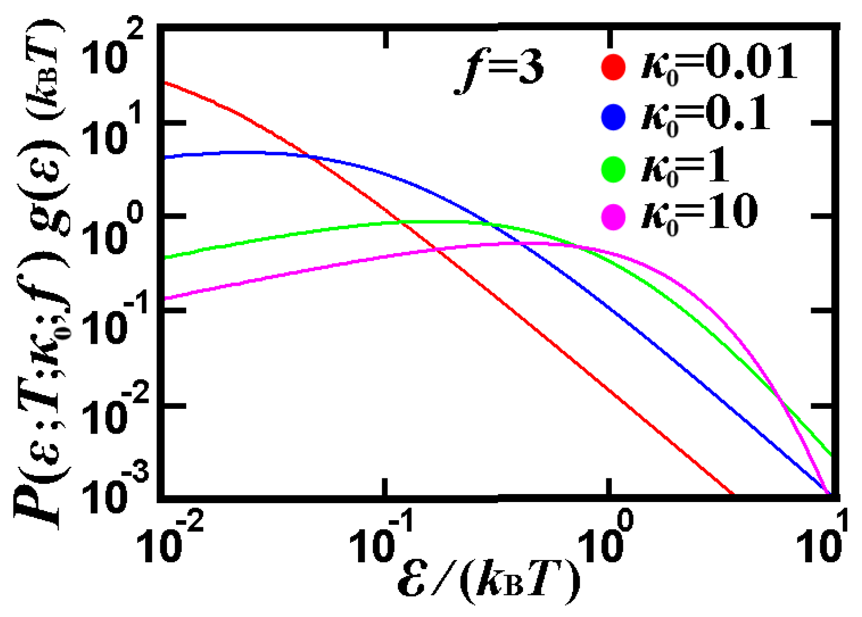
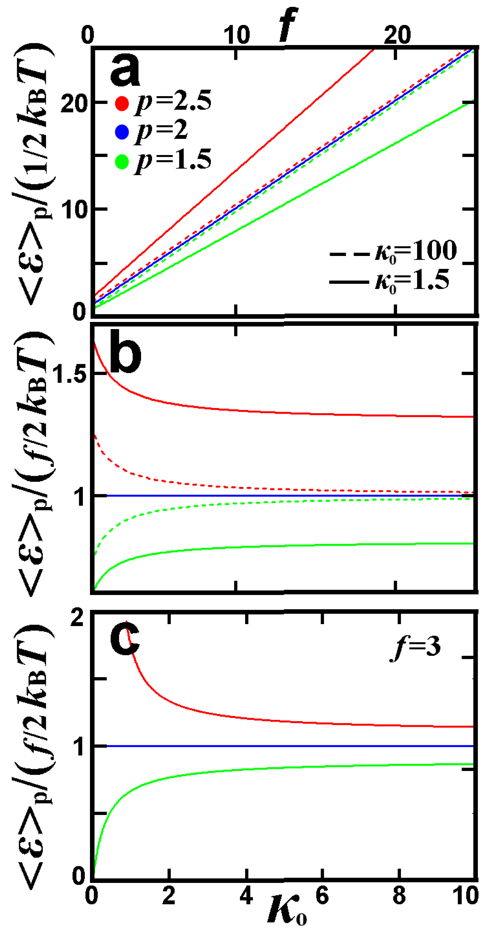
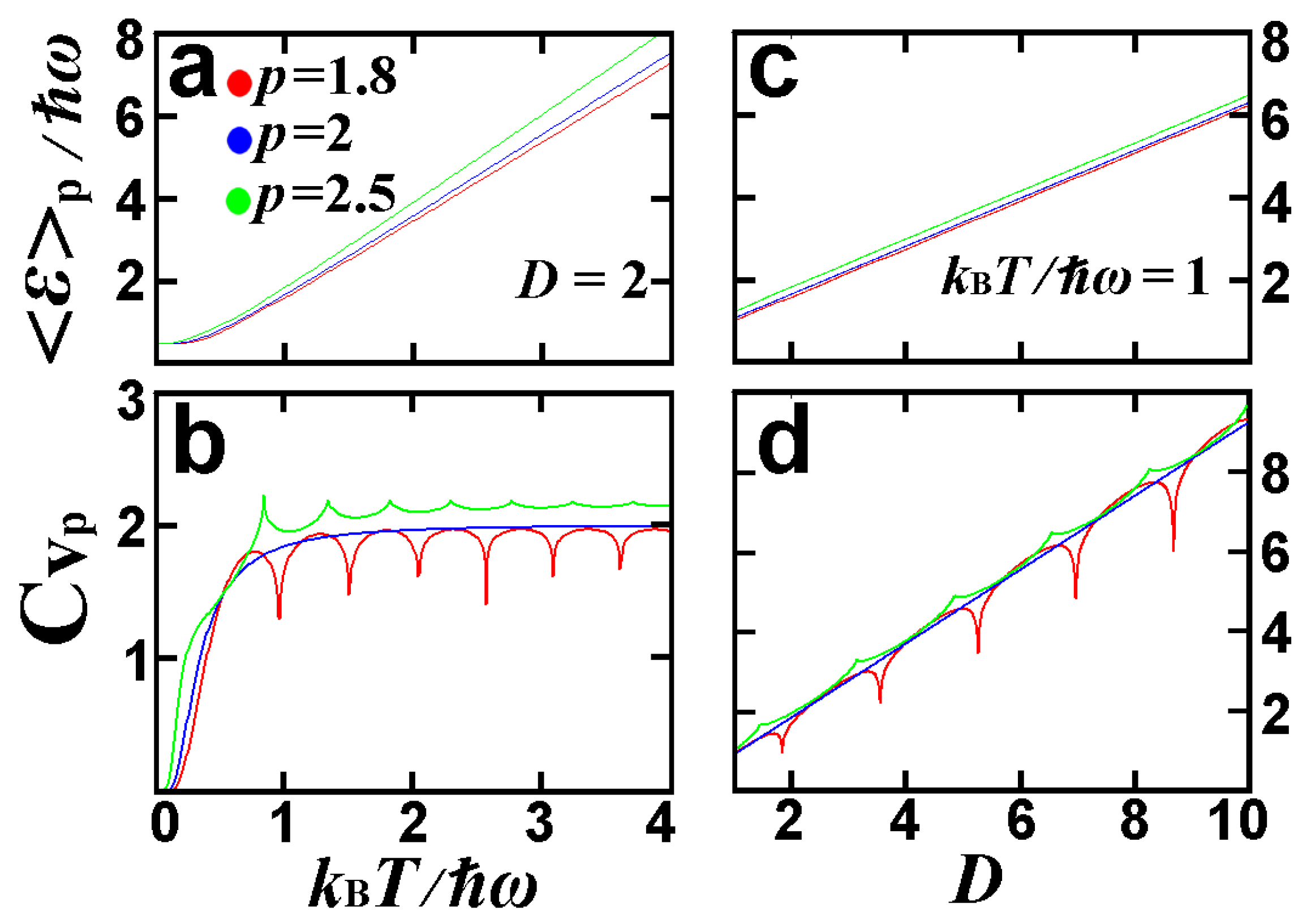
3.3.3. D-Dimensional Quantum Harmonic Oscillator in Thermal Equilibrium

For the energy states { ε n } n = 1 W with degeneracy { g n } n = 1 W that are associated with the discrete energy distribution { p n } n = 1 W , the L p internal energy ε p is
n = 1 W p n g n | ε n - ε p | p - 1 s i g n ( ε n - ε p ) = 0
with the Boltzmann’s energy distribution p n e - ε n k B T at thermal equilibrium. The D-dimensional quantum harmonic oscillator has discrete energy spectrum ε n = ω ( n + 1 2 ) with degeneracy g n = ( n n + D - 1 ) ( n + D - 1 ) ! / n ! , n = 0 , 1 , 2 , ... Then, the internal energy ε p is implicitly given by
n = 0 e - ω k B T n · | n + 1 2 - ε p ω | p - 1 s i g n n + 1 2 - ε p ω · ( n + D - 1 ) ! n ! = 0
In Figure 3a, we depict ε p / ( ω ) with respect to k B T / ( ω ) , for p = 1 . 8 , 2 , 2 . 5 and D = 2 . The relevant heat capacity, c V , p = ( ε p / T ) V , is shown in Figure 3b. For high temperatures, the Dulong–Petit limit is generalized to ε p 1 2 f p · k B T + α p · ω , and heat capacity c V , p 1 2 f p · k B , where the reflected degrees of freedom are f p 2 D + 0 . 6 · ( p - 2 ) ; the involved constant is α p 0 . 015 D ( p - 2 ) . Each dimension of the Euclidean quantum oscillator has two degrees of freedom so that f 2 = 2 D ; the non-Euclidean quantum oscillator deviates proportionally to the factor f p - f 2 p - 2 . In Figure 3c,d we depict ε p and c V , p as a function of the dimensionality D, for p = 1 . 8 , 2 , 2 . 5 and k B T / ( ω ) = 1 . While for the Euclidean norm the heat capacity gives c V , p / k B = D , for the sub- and super-Euclidean norms we have c V , p / k B < D and > D , respectively. Finally, we remark that the heat capacity appears to have periodic cusps that become smaller in higher temperatures.
Figure 2. The dependence of the internal energy on the degrees of freedom f and the kappa index κ 0 . (a) Plot of ε p / ( 1 / 2 k B T ) vs. the degrees of freedom f, for p = 1 . 5 (red), 2 (blue), 2 . 5 (green), and κ 0 = 1 . 5 (solid), and 100 (dash). (b) Plot of ε p / ( f / 2 k B T ) , vs. f, for the same p and κ 0 . (c) The same plot as (b), but vs. κ 0 and for f = 3 . We observe larger deviation from the Euclidean norm for smaller kappa indices. Note that the graph is restricted to κ 0 > p - 2 (see text).
Entropy 14 02375 g002
Figure 3. The internal energy and heat capacity of the D-dimensional quantum harmonic oscillator for non-Euclidean norms ( p ) at thermal equilibrium ( κ 0 ). (a), (b) The internal energy ε p / ( ω ) and heat capacity c V , p , are respectively plotted vs. the temperature k B T / ( ω ) , for p = 1 . 8 (red), 2 (blue), 2 . 5 (green), and D = 2 . (c), (d) Similar to (a) and (b), but plotted as functions of the dimensionality D, for k B T / ( ω ) = 1 .
Entropy 14 02375 g003

4. The Non-Euclidean L p -Variance of the L p -Expectation Value

4.1. Preliminaries: Formulations

We study the L p -variance, defined either in the discrete description { y k } k = 1 W , y k D y R , k = 1 , , W , with probability distribution { p k } k = 1 W ,
σ 2 p = k = 1 W p k | y k - y p | p ( p - 1 ) k = 1 W p k | y k - y p | p - 2
with y p implicitly given by Equation (8), or in the continuous description y D y R , with probability distribution p ( y ) ,
σ 2 p = y D y p ( y ) | y - y p | p d y ( p - 1 ) y D y p ( y ) | y - y p | p - 2 d y
with y p implicitly given by
y D y p ( y ) | y - y p | p - 1 s i g n ( y - y p ) d y = 0

4.2. Examples

4.2.1. Example 1: Gaussian distribution

Consider the Gaussian probability distribution density
f G ( y ; μ , σ ) = 1 2 π 1 σ e - 1 2 σ 2 ( y - μ ) 2
Then, the L p variance is given by
σ 2 p = - + | y - μ | p e - 1 2 σ 2 ( y - μ ) 2 d y ( p - 1 ) - + | y - μ | p - 2 e - 1 2 σ 2 ( y - μ ) 2 d y = σ 2 p - 1 - + | u | p e - 1 2 u 2 d u - + | u | p - 2 e - 1 2 u 2 d u =
σ 2 p - 1 0 + u p e - 1 2 u 2 d u 0 + u p - 2 e - 1 2 u 2 d u = σ 2 2 p - 1 0 + z p + 1 2 - 1 e - z d z 0 + z p - 1 2 - 1 e - z d z = σ 2 2 p - 1 Γ ( p + 1 2 ) Γ ( p - 1 2 ) = σ 2
where we have set u y - μ σ , and z u 2 2 . Thus, the L p variance yields the well-known Euclidean variance σ 2 of the Gaussian distribution.

4.2.2. Example 2: Generalized Gaussian distribution

Consider the Generalized Gaussian probability distribution density,
f G G ( y ; μ , σ ; Q , p ) = C Q , p 1 σ e - η Q , p | y - μ σ | Q
where Q 0 is the shape parameter, C Q , p is the normalization constant, and η Q , p is calculated by setting σ 2 p σ 2 ,
σ 2 p = - + | y - μ | p e - η Q , p | y - μ σ | Q d y ( p - 1 ) - + | y - μ | p - 2 e - η Q , p | y - μ σ | Q d y = σ 2 p - 1 - + | u | p e - η Q , p | u | Q d u - + | u | p - 2 e - η Q , p | u | Q d u =
σ 2 p - 1 0 + u p e - η Q , p u Q d u 0 + u p - 2 e - η Q , p u Q d u = σ 2 η Q , p - 2 Q p - 1 0 + z p + 1 Q - 1 e - z d z 0 + z p - 1 Q - 1 e - z d z = σ 2 η Q , p - 2 Q p - 1 Γ ( p + 1 Q ) Γ ( p - 1 Q ) = σ 2
where we have set u y - μ σ , z η Q , p u Q , and
η Q , p 1 p - 1 Γ ( p + 1 Q ) Γ ( p - 1 Q ) Q 2
Of particular interest is the case where the shape parameter equals the norm, Q = p , namely,
f G G ( y ; μ , σ ; p ) = C p 1 σ e - η p | y - μ σ | p
with
η p = 1 p - 1 Γ ( 1 + 1 p ) Γ ( 1 - 1 p ) p 2 = sin ( π p ) Γ ( 1 p ) 2 π p ( p - 1 ) p 2
(Note that y p = μ for both the examples. See Section 5.1.)

4.3. Justification of the L p -Variance Expression

Let the set of { Y i } i = 1 N independent and identically distributed random variables with sampling values { y i } i = 1 N , y i D y R , i = 1 , , N .
First, we consider that each variable is distributed as Y i N ( μ , σ ) , namely, by the Gaussian probability distribution density
f G ( y i ; μ , σ ) = 1 2 π 1 σ e - 1 2 σ 2 ( y i - μ ) 2
i = 1 , , N . Then, the likelihood function is constructed
L y ( { y i } i = 1 N ; μ , σ ) = i = 1 N f G ( y i ; μ , σ ) = ( 2 π σ ) - N e - 1 2 σ 2 i = 1 N ( y i - μ ) 2
ln [ L y ( { y i } i = 1 N ; μ , σ ) ] = - N 2 ln ( 2 π ) - N ln σ - 1 2 σ 2 i = 1 N ( y i - μ ) 2
Then, μ ln [ L y ( { y i } i = 1 N ; μ ; σ ) ] = 0 leads to
i = 1 N y i - μ = 0 μ = 1 N i = 1 N y i
while σ ln [ L y ( { y i } i = 1 N ; μ ; σ ) ] = 0 leads to
- N 1 σ + 1 σ 3 i = 1 N y i - μ 2 = 0 σ 2 = 1 N i = 1 N y i - μ 2
Thus, for the normally distributed { y i } i = 1 N , the best estimators for the true value of the parameters μ and σ 2 are the Euclidean estimators of the mean and variance, that is μ ^ 2 , N ( { y i } i = 1 N ) = 1 N i = 1 N y i and σ 2 ^ 2 , N ( { y i } i = 1 N ) = 1 N i = 1 N y i - μ 2 , respectively. What is important here is not the variance σ 2 of the theoretical distribution density f G ( y i ; μ ; σ ) , but the variance S 2 ^ 2 , N of the Euclidean mean estimator μ ^ 2 , N ( { y i } i = 1 N ) [31], given by
1 S 2 ^ 2 , N = - 2 μ 2 ln [ L y ( { y i } i = 1 N ; μ ; σ ) ] = N 1 σ 2 = N 1 σ 2 ^ 2 , N
so that the value of μ, estimated by μ ^ 2 , N , has a variance S 2 ^ 2 , N , given by
S 2 ^ 2 , N = 1 N σ 2 ^ 2 , N
Now consider that each variable is distributed as Y i GG ( μ , σ ; Q , p ) , namely, by the General Gaussian probability distribution density of Equation (35),
f G G ( y i ; μ , σ ; p ) = C p 1 σ e - η p | y i - μ σ | p
i = 1 , , N . Then, the likelihood function is constructed
L y ( { y i } i = 1 N ; μ , σ ; p ) = i = 1 N f G G ( y i ; μ , σ ; p ) = C p N σ - N e - η p σ p i = 1 N | y i - μ | p
ln [ L y ( { y i } i = 1 N ; μ , σ ; p ) ] = N ln C p - N ln σ - η p σ p i = 1 N | y i - μ | p
Then, μ ln [ L y ( { y i } i = 1 N ; μ , σ ; p ) ] = 0 leads to
i = 1 N y i - μ p - 1 s i g n ( y i - μ ) = 0
Thus, for { y i } i = 1 N distributed by the General Gaussian, the best estimator for the true value of the parameter μ is the non-Euclidean L p -mean estimator μ ^ p , N ( { y i } i = 1 N ; p ) , defined in Equation (19).
In addition, σ ln [ L y ( { y i } i = 1 N ; μ , σ ; p ) ] = 0 leads to
- N 1 σ + η p p σ p + 1 i = 1 N y i - μ p = 0 σ p η p p = 1 N i = 1 N y i - μ p
and thus, the variance S 2 ^ p , N of the estimator μ ^ p , N ( { y i } i = 1 N ; p ) is given by
1 S 2 ^ p , N = - 2 μ 2 ln [ L y ( { y i } i = 1 N ; μ , σ ; p ) ] = η p p σ p ( p - 1 ) i = 1 N y i - μ p - 2 = N ( p - 1 ) i = 1 N y i - μ p - 2 i = 1 N y i - μ p N 1 σ 2 ^ p , N
or
S 2 ^ p , N = 1 N σ 2 ^ p , N
which is similar to Equation (43) after replacing the Euclidean variance, σ 2 ^ 2 , N , with the non-Euclidean one, σ 2 ^ p , N . Finally, the L p variance (e.g., as given in Equation (30)) can be written in the form of Equation (17), i.e.,
σ 2 p = k = 1 W p k | y k - y p | p ( p - 1 ) k = 1 W p k | y k - y p | p - 2 = k = 1 W p k ( y k - y p ) | y k - y p | p - 1 s i g n ( y k - y p ) ( p - 1 ) ϕ p = k = 1 W p k ( y k - y p ) L ^ p ( y k - y p ) = ( y - y p ) L ^ p ( y - y p ) 2 .
Note that the L p mean y p (Equations (1) and (8)) is derived from the minimization of σ 2 p ( α ) = 1 ( p - 1 ) ϕ p T D p ( { y k } k = 1 W ; α ; p ) p , which is proportional to the total deviations T D p p (Equation (2)).
Moreover, total deviations T D p ( { y k } k = 1 W ; α ; p ) can be expanded at the minimum α = α * ,
T D p ( { y k } k = 1 W ; α ; p ) p = A 0 ( p ) + A 1 ( p ) ( α - α * ) + A 2 ( p ) ( α - α * ) 2 + O [ ( α - α * ) 3 ]
where A 0 ( p ) = T D p , M i n ( { y k } k = 1 W ; p ) p = k = 1 W p k | y k - α * ( p ) | p is the Total p-Deviations minimum value, A 1 ( p ) = - p k = 1 W p k | y k - α * ( p ) | p - 1 s i g n ( y k - α * ( p ) ) = 0 is the Total p-Deviation first derivative (in terms of the parameter α), which is equal to zero, while the curvature factor A 2 ( p ) is given by
A 2 ( p ) = p ( p - 1 ) 2 k = 1 W p k | y k - α * ( p ) | p - 2
As it is shown in [7], the variance σ 2 p that is proportional to the square error of the optimal value α * ( p ) is inversely proportional to A 2 ( p ) ,
σ 2 p 1 ( p - 1 ) k = 1 W p k | y k - α * ( p ) | p - 2
On the other hand, it is expected that the variance σ 2 p will be proportional also to A 0 ( p ) , namely,
σ 2 p k = 1 W p k | y k - α * ( p ) | p
which completes the proportionality of Equation (51), leading to Equation (30).
There are two more ways to show the specific expression of L p -variance: The proportionality factor C connects, either the variance with the Total Deviations, i.e., σ 2 p = C · T D p p , or the energy states { ε k } k = 1 W with the “ L p energy states” { L ^ p ( ε k ) } k = 1 W , i.e., L ^ p ( ε k - U p ) = C | ε k - U p | p - 1 s i g n ( ε k - U p ) . The property (ii) of the non-Euclidean norm operator L ^ p holds if and only if C = 1 ( p - 1 ) ϕ p . This can be shown in the following two ways: (1) Due to the property (ii) of the non-Euclidean norm operator, the respective Canonical probability distribution can be automatically derived. Indeed, the internal energy constraint ε p = k = 1 W p k L ^ p ( ε k ) leads to the derivative p j k = 1 W p k L ^ p ( ε k ) = L ^ p ( ε j ) , so that by maximizing Boltzmann-Gibbs entropy we end up with p k e - β L ^ p ( ε k ) . (2) The connection with thermodynamics can be achieved if and only if C = 1 ( p - 1 ) ϕ p (Equation (15)).

5. Further Analytical and Numerical Examples

5.1. Analytical Example: The Spectrum of the L p Means and Its Degeneration

For a continuous description of data y ( t ) D y R , where t D t R is a continuous index, the L p -expectation value y p is given by
t D t | y ( t ) - y p | p - 1 s i g n [ y ( t ) - y p ] d t = 0
Given the probability distribution of y-values, p ( y ) , the L p -expectation value is given by Equation (32). Consider now the equidistribution of data in the interval [ 0 , 1 ] . From Equation (32) we have
0 1 | y - y p | p - 1 s i g n ( y - y p ) d y = 0 0 y p ( y p - y ) p - 1 d y = y p 1 ( y - y p ) p - 1 d y y p p = ( 1 - y p ) p y p = 1 2 p 1 .
The fact that y p is independent of p, is a general result of symmetric probability distributions. Indeed, consider a distribution p ( y ) , y [ - c , c ] , symmetric at y = 0 , i.e., p ( - y ) = p ( y ) y [ - c , c ] . Then,
- c c p ( y ) | y | p - 1 s i g n ( y ) d y = 0 ,
(the sign is odd function, while p ( y ) | y | p - 1 is even). Hence, given the uniqueness of y p for a given p, we conclude in y p = 0 , p 1 .
Therefore, in the case where the distribution p ( y ) is symmetric, the whole set of y p -values degenerate to one single value, which can be found thus, by the usual Euclidean norm, namely y p = y 2 . (The opposite statement is also true.) However, when p ( y ) is asymmetric, a spectrum-like range of different y p -values is generated [7]. For example, the distribution p ( y ) 1 + δ ( 1 - 3 y 2 ) in the interval y [ 0 , 1 ] is symmetric for δ = 0 , but becomes asymmetric for 0 < δ < < 1 . Then, we find y p 1 2 - 3 4 1 p + 1 δ + O δ 2 .

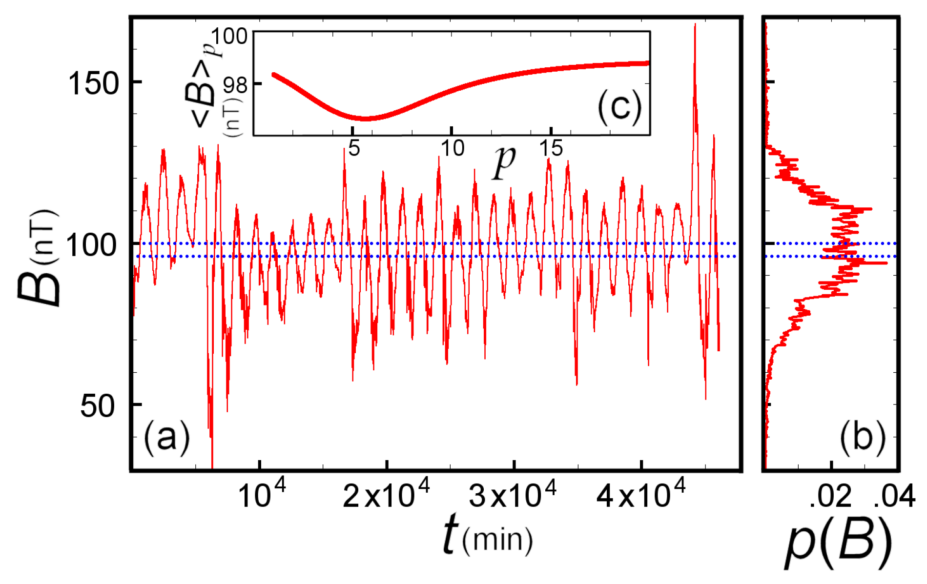
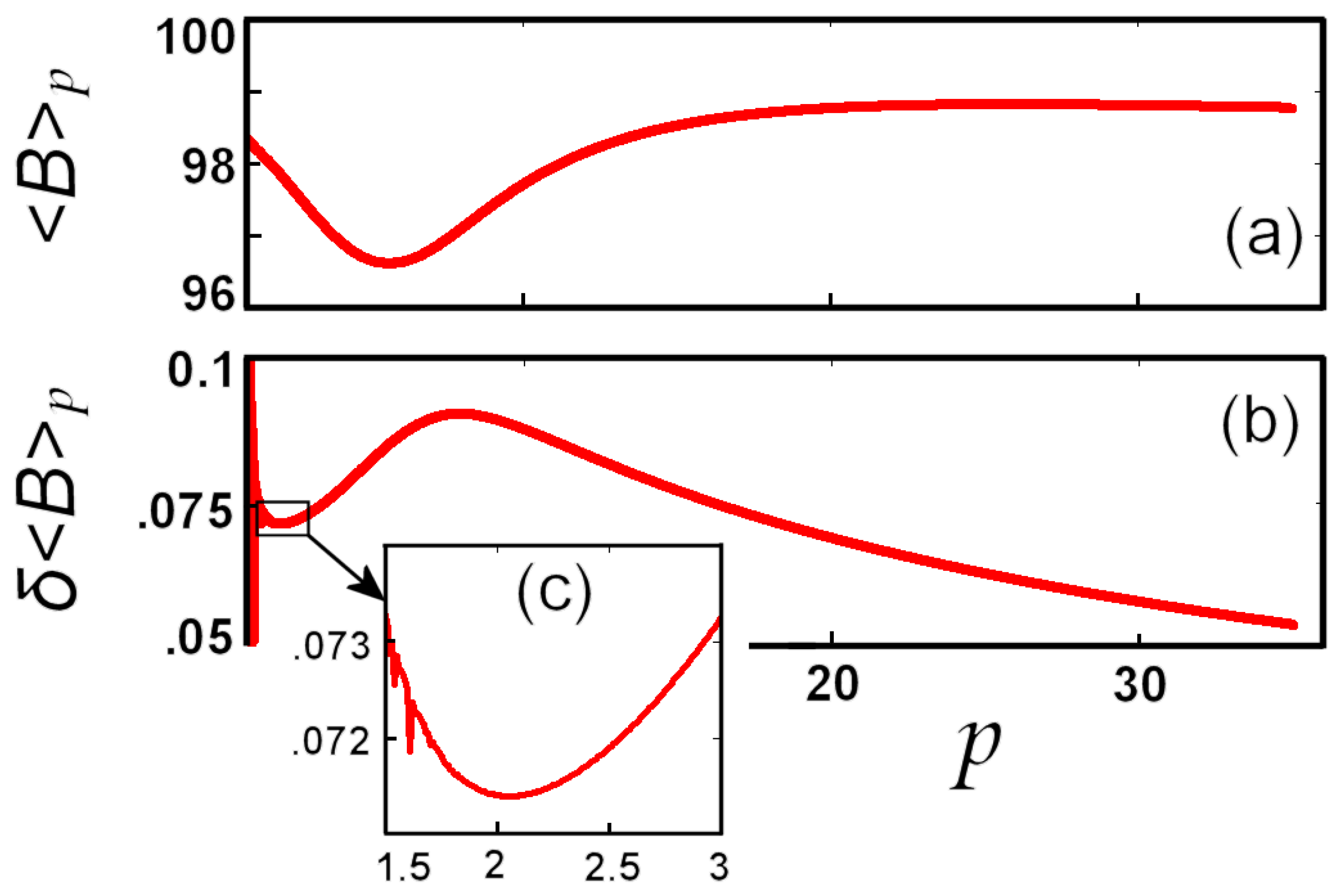
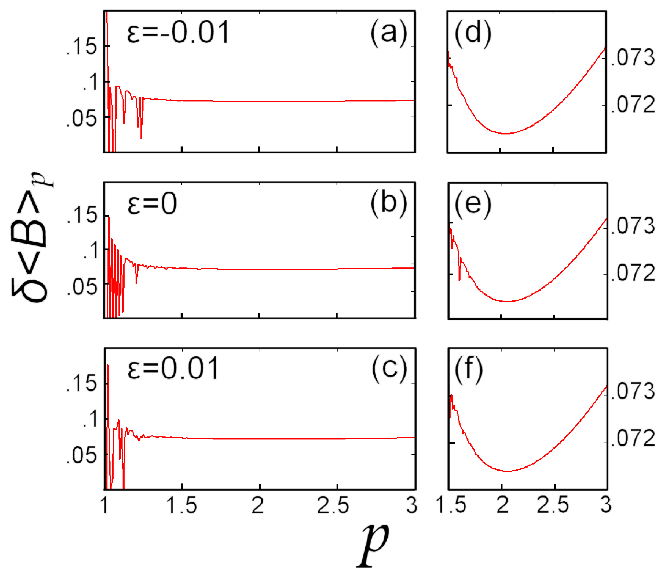
5.2. Numerical Example: Earth’s Magnetic Field

We consider the time series of the Earth’s magnetic field magnitude (in nT). In particular, we focus on a stationary segment recorded by the GOES-12 satellite between the month 1/1/2008 and 1/2/2008, that is a sampling of one measurement per minute, constituting a segment of N = 46 , 080 data points, depicted in Figure 4a. This segment is characterized by a roughly symmetric distribution p ( B ) (in nT - 1 ), depicted in Figure 4b, resulting to a narrow spectrum of B p -values, depicted in Figure 4c. Notice that the extreme values of B p do not coincide with the respective for p = 1 and p . Indeed, a minimum of the L p -expectation values, that is B p , m i n 96 . 614 nT, can be found for the non-Euclidean norm p 5 . 63 , while a maximum value of about B p , m a x 98 . 819 nT, is located at p 25 . 83 . As p , B p tends to ( B m i n + B m a x ) / 2 98 . 535 nT. Hence, it is evident that L p means μ p are not indispensably monotonic functions of p.
Figure 4. The magnitude of the Earth’s total magnetic field. (a) The time series recorded between 1/1/2008 and 1/2/2008. (b) The relevant distribution p ( B ) is roughly symmetric. As a result, the numerically calculated L p -expectation values, B p , configure a narrow spectrum within the interval between the two horizontal dotted lines, where the dependence of B p -values on the p-norm is shown within the magnified inset (c).
Entropy 14 02375 g004
The expectation value B p is given by the estimator μ ^ p , N ( { B i } i = 1 N ; p ) . On the other hand, the error δ B p is given by the square root of the variance S 2 ^ p , N of the estimator μ ^ p , N ( { B i } i = 1 N ; p ) , that is
δ B p = S ^ p , N = 1 N σ ^ p , N = 1 N 1 p - 1 i = 1 N B i - B p p i = 1 N B i - B p p - 2
In Figure 5a,b, the L p -expectation value of the Earth’s magnetic field magnitude (shown in Figure 4a), B p , together with its error δ B p , are respectively depicted as functions of the p-norm. A local minimum of the error δ B p can be detected for p 2 . 05 , for which B p 97 . 88 nT and δ B p , m i n 0 . 071 nT, shown in the magnified inset of Figure 5c.
Figure 5. The L p -expectation value of the magnitude of the Earth’s total magnetic field (shown in Figure 4a), B p , together with its error δ B p , are depicted as functions of the p-norm (panels (a) and (b), respectively). A local minimum of the error is found close to the Euclidean norm, i.e., for p 2 . 05 , as it is shown within the magnified inset (c).
Entropy 14 02375 g005
For p 2 . 05 the error increases as p increases, until it reaches a local maximum at p 7 . 88 , for which B p 97 . 07 nT and δ B p , m a x 0 . 091 nT. Then, for p 7 . 88 the error decreases monotonically as p increases. We can readily derive that δ B p 1 2 ( B m a x - B m i n ) 1 N 1 p - 1 0 , as p .
For p 2 . 05 the error increases as p decreases, but numerous fluctuations appear that become more dense as p 1 . This “instability cloud” is due to the reading errors of the data values, with their effect being magnified as p - 1 tends to zero. This effect can be demonstrated in Figure 6, where the error δ B p is depicted when an additive noise is inserted into the { B i } i = 1 N values. In particular, we consider the perturbed values { B ˜ i } i = 1 N , where B ˜ i B i + ϵ r i , i = 1 , , N , with { r i } i = 1 N , being equidistributed in [ 0 , 1 ] and | ϵ | is the amplitude of the perturbations. We set | ϵ | = 0 . 01 nT, which is equal to the resolution (reading error) of the values { B i } i = 1 N . In Figure 6a we set ϵ = - 0 . 01 nT, while in Figure 6c we set ϵ = + 0 . 01 nT. In Figure 6b we depict the unperturbed error for convenience. We observe that the “instability cloud”, occurred for p 1 , is different for the three cases ϵ = - 0 . 01 , 0, and + 0 . 01 (nT). However, the minimum at p 2 . 05 remains unaffected.
The existence of a local minimum of the error, such as the minimum at p 2 . 05 , is of great importance. It suggests that for this specific norm, the expectation value comes with the minimum error. Therefore, after the total deviations minimization that leads to the normal Equation (1) from which the optimal parameter α * ( p ) is derived, the optimization is completed by determining the specific norm p * for which the variance σ 2 ^ p ( p ) has a local minimum (if that exists). The importance of the local minimum of σ 2 p ( p ) is that for any deviation of the norm at p = p * , either p < p * , or p > p * , the error increases, introducing thus, a type of norm-stability. Hence, the L p -norm that corresponds to the minimized error, p 2 . 05 , is distinguished. It is interesting that the norm p 2 . 05 is very close to the Euclidean one ( p = 2 ). However, it has to be stressed out that there is not any universally preferred norm, since this is dependent on the specific data values.
Both the diagrams of the L p mean μ p ( p ) and its relevant error δ μ p ( p ) , depicted in terms of the norm p, constitute a “metricogram". In a metricogram, we are able to observe the whole spectrum of the L p mean and its error, and to recognize the preferable norms.
Figure 6. The error δ B p is depicted with additive equidistributed noise inserted into the { B i } i = 1 N values ( N = 46080 ). The amplitude of the noise is equal to the resolution of the values { B i } i = 1 N . Namely, we set ϵ = - 0 . 01 nT (a), and ϵ = + 0 . 01 nT (c). In panel (b) we depict the unperturbed error for convenience. The magnified panels (d), (e) and (f) of the respective panels (a), (b) and (c) demonstrate the minimum error at p 2 . 05 that remains unaffected, for amplitudes of additive noise less or equal to the reading error, i.e., | ϵ 0 . 01 | nT, in contrast to the fluctuations, appearing for p - 1 0 , which are affected by the additive noise.
Entropy 14 02375 g006

6. Conclusions

This analysis introduced a possible generalization of the basic statistical concepts of the expectation value and variance for non-Euclidean metrics induced by L p norms. The Euclidean L 2 mean is derived by minimizing the sum of the total square deviations T S D , which is the Euclidean variance. Similarly, the non-Euclidean L p means were developed by minimizing the sum of the L p deviations T D p p , which is proportional to the L p variance. The main advantage of the new statistical approach is that the p-norm is a free parameter, thus both the L p -normed expectation values and their variance are flexible to analyze new phenomena that cannot be described under the notions of classical statistics based on Euclidean norms.
As it was shown, the L p means embody a generic formal scheme of means characterization, given the sampling values { y i } i = 1 N . This involves the existence of a univalued, N-multivariable function M ( { y i } i = 1 N ) , fulfilling the following three preconditions: (i) Continuity; (ii) Internness; (iii) Symmetry. (This axiomatic scheme of means characterization generalizes the one proposed by Aczél [23], which led to the Euclidean φ -means.)
The L p expectation values can be expressed in terms of the operator L ^ p , which helps to automatically retrieve the non-Euclidean representation of a given formulation, for which the Euclidean representation is known. This idea was utilized to derive the L p -variance σ 2 p , the derivative β y p (with respect to a parameter β, y p = y p ( β ) ), and the novel representation of several fundamental notions of Statistical Mechanics (based on the L p -norm), e.g., Canonical probability distribution and partition function.
The L p -mean estimator, μ ^ p , N = μ ^ p , N ( { y i } i = 1 N ; p ) , of a sampling values { y j } j = 1 N of the independent and identically distributed random variables { Y i } i = 1 N was defined. It is characterized by the following properties: (i) μ ^ p , N ( { y i } i = 1 N ; p ) p = μ p , and (ii) μ ^ p , N μ p as N , where μ p is the L p -expectation value of each of the { Y i } i = 1 N random variables. These properties are similar to the known Euclidean ones, namely, (i) 1 N i = 1 N y i 2 = μ 2 , and (ii) 1 N i = 1 N y i μ 2 as N .
The expression of the L p variance σ 2 p was shown by four different ways: (a) The maximization of the likelihood function, constructed by N independent and identically distributed random variables { Y i } i = 1 N , led to the L p -mean estimator μ ^ p , N and its L p variance σ 2 ^ p , N , if Y i GG ( μ , σ ; p ) , i = 1 , , N , namely, the random variables are distributed according to the General Gaussian distribution with shape parameter equal to the p-norm. (b) The variance σ 2 p is proportional to the total deviations (residuals) A 0 ( p ) (Equation (49)), and to the inverse of the curvature factor A 2 ( p ) , given in Equation (50). The next two ways utilize the fact that the property (ii) of the operator L ^ p holds if and only if the proportionality factor C, that connects, either the variance with the Total p-Deviations, i.e., σ 2 p = C · T D p p , or the energy states { ε k } k = 1 W with the “ L p energy states” { L ^ p ( ε k ) } k = 1 W , i.e., L ^ p ( ε k - U p ) = C | ε k - U p | p - 1 s i g n ( ε k - U p ) , is given by the one single expression C = 1 ( p - 1 ) ϕ p : (c) Derivation of the Canonical probability distribution of L p -normed Statistical Mechanics. (d) Connection with thermodynamics, e.g., U p = - ln Z p β .
We remark the difference between the extracted expression of the L p deviation σ p , and the one considered in the literature, σ ˜ p , that is
σ p = 1 p - 1 k = 1 W p k | y k - y p | p k = 1 W p k | y k - y p | p - 2 , σ ˜ p = k = 1 W p k | y k - y 2 | p p
which is supposed to represent the generalization of σ 2 = k = 1 W p k | y k - y 2 | 2 . The correct expressions of the L p means and variance can be crucial for providing insights into the fundamental numerical tools of data analysis, such as the moving averages techniques for smoothing, the multifractal detrended fluctuation analysis (MF-DFA) (e.g., see [32,33]), the singular spectrum analysis technique [34], etc. Having found a new class for the mean and variance, it is straightforward to develop an unbiased estimator for the population coefficient of variation (e.g., for Euclidean norm, see [35]).
Several analytical and numerical examples were examined. When the distribution of the data values is symmetric, the whole set of L p means degenerates to one single value, while when it is asymmetric, a spectrum-like range of L p means is generated. In addition, we dealt with the numerical data of the Earth’s magnetic field magnitude.
The mean value is uniquely defined and dependent on the p-norm. The error of the mean is also dependent on the p-norm, leading to a variant weight of the mean (inverse square). In a metricogram, we observe the whole spectrum of the L p mean μ p ( p ) and its relevant error δ μ p ( p ) , depicted in terms of the p-norm, where we can detect any preferable norms. For example, for the numerical example of the Earth’s magnetic field magnitude (time series recorded within January of 2008), a preferable norm was found for p 2 . 05 , for which p δ B p ( p ) = 0 , 2 p 2 δ B p ( p ) > 0 .
The classical concept of expectation values was generalized to the non-Euclidean L p -normed representation, highlighting its implication in Statistical Mechanics. Indeed, the L p expectation value of a given energy spectrum { ε k } k = 1 W represents the non-Euclidean adaptation of the internal energy U p . This is an issue that has to be considered in Statistical Mechanics: Several pedagogical examples were examined: gas in thermal equilibrium, space plasmas out of thermal equilibrium, and multi-dimensional quantum harmonic oscillator at thermal equilibrium.

References

  1. Abramowitz, M.; Stegun, I.A. Handbook of Mathematical Functions; Dover Publications: New York, NY, USA, 1965. [Google Scholar]
  2. Kolmogorov, A.N. Sur la notion de la moyenne (in French). Atti Accad. Naz. Lincei 1930, 12, 388–391. [Google Scholar]
  3. Nagumo, M. Uber eine Klasse der Mittelwerte (in German). Jpn. J. Math. 1930, 7, 71–79. [Google Scholar]
  4. Hardy, G.H.; Littlewood, J.E.; Pólya, G. Inequalities; Cambridge University Press: Cambridge, UK, 1934. [Google Scholar]
  5. Ben-Tal, A. On generalized means and generalized convex functions. J. Optimiz. 1977, 21, 1–13. [Google Scholar] [CrossRef]
  6. Páles, Z. On the characterization of quasi arithmetic means with weight function. Aequationes Math. 1987, 32, 171–194. [Google Scholar] [CrossRef]
  7. Livadiotis, G. Approach to block entropy modeling and optimization. Physica A 2008, 387, 2471–2494. [Google Scholar] [CrossRef]
  8. Bajraktarevic, M. Sur un equation fonctionelle aux valeurs moyens (in French). Glas. Mat.-Fiz. Astronom. 1958, 13, 243–248. [Google Scholar]
  9. Aczél, J.; Daroczy, Z. On Measures of Information and Their Characterization; Academy Press: New York, NY, USA, 1975. [Google Scholar]
  10. Norries, N. General means and statistical theory. Am. Stat. 1976, 30, 8–12. [Google Scholar]
  11. Kreps, D.M.; Porteus, E.L. Temporal resolution of uncertainty and dynamic choice theory. Econometrica 1978, 46, 185–200. [Google Scholar] [CrossRef]
  12. Flandrin, P. Separability, positivity, and minimum uncertainty in time-frequency energy distributions. J. Math. Phys. 1998, 39, 4016–4039. [Google Scholar] [CrossRef]
  13. Czachor, M.; Naudts, J. Thermostatistics based on Kolmogorov–Nagumo averages: Unifying framework for extensive and nonextensive generalizations. Phys. Lett. A 2002, 298, 369–374. [Google Scholar] [CrossRef]
  14. Dukkipati, A.; Narasimha-Murty, M.; Bhatnagar, S. Uniqueness of nonextensive entropy under Renyi’s recipe. Comp. Res. Rep. 2005, 511078. [Google Scholar]
  15. Tzafestas, S.G. Applied Control: Current Trends and Modern Methodologies; Electrical and Computer Engineering Series; Marcel Dekker, Inc.: New York, 1993. [Google Scholar]
  16. Koch, S.J.; Wang, M.D. Dynamic force spectroscopy of protein-DNA interactions by unzipping DNA. Phys. Rev. Lett. 2003, 91, 028103. [Google Scholar] [CrossRef] [PubMed]
  17. Still, S.; Kondor, I. Regularizing portfolio optimization. New J. Phys. 2010, 12, 075034. [Google Scholar] [CrossRef]
  18. Livadiotis, G. Approach to general methods for fitting and their sensitivity. Physica A 2007, 375, 518–536. [Google Scholar] [CrossRef]
  19. Bavaud, F. Aggregation invariance in general clustering approaches. Adv. Data Anal. Classif. 2009, 3, 205–225. [Google Scholar] [CrossRef]
  20. Gajek, L.; Kaluszka, M. Upper bounds for the L1-risk of the minimum L1-distance regression estimator. Ann. Inst. Stat. Math. 1992, 44, 737–744. [Google Scholar] [CrossRef]
  21. Huber, P. Robust Statistics; John Wiley & Sons: New York, NY, USA, 1981. [Google Scholar]
  22. Hampel, F.R.; Ronchetti, E.M.; Rousseeuw, P.J.; Stahel, W.A. Robust Statistics. The Approach Based on Influence Functions; John Willey & Sons: New York, NY, USA, 1986. [Google Scholar]
  23. Aczél, J. On mean values. Bull. Amer. Math. Soc. 1948, 54, 392–400. [Google Scholar] [CrossRef]
  24. Aczél, J. Lectures on Functional Equations and Their Applications; Academy Press: New York, NY, USA, 1966. [Google Scholar]
  25. Toader, G.; Toader, S. Means and generalized means. J. Inequal. Pure Appl. Math. 2007, 8, 45. [Google Scholar]
  26. Livadiotis, G.; McComas, D.J. Beyond kappa distributions: Exploiting Tsallis statistical mechanics in space plasmas. J. Geophys. Res. 2009, 114, A11105. [Google Scholar] [CrossRef]
  27. Tsallis, C. Introduction to Nonextensive Statistical Mechanics; Springer: New York, NY, USA, 2009. [Google Scholar]
  28. Livadiotis, G.; McComas, D.J. Invariant kappa distribution in space plasmas out of equilibrium. Astrophys. J. 2011, 741, 88. [Google Scholar] [CrossRef]
  29. Livadiotis, G.; McComas, D.J. Measure of the departure of the q-metastable stationary states from equilibrium. Phys. Scripta 2010, 82, 035003. [Google Scholar] [CrossRef]
  30. Livadiotis, G.; McComas, D.J. Exploring transitions of space plasmas out of equilibrium. Astrophys. J. 2010, 714, 971. [Google Scholar] [CrossRef]
  31. Melissinos, A.C. Experiments in Modern Physics; Academic Press Inc.: London, UK, 1966; pp. 438–464. [Google Scholar]
  32. Kantelhardt, J.; Zschiegner, S.A.; Koscielny-Bunde, E.; Bunde, A.; Havlin, S.; Stanley, H.E. Multifractal detrended fluctuation analysis of nonstationary time series. Physica A 2002, 316, 87–114. [Google Scholar] [CrossRef]
  33. Varotsos, P.A.; Sarlis, N.V.; Skordas, E.S. Attempt to distinguish electric signals of a dichotomous nature. Phys. Rev. E 2003, 68, 031106. [Google Scholar] [CrossRef]
  34. Hassani, H.; Thomakos, D. A review on singular spectrum analysis for economic and financial time series. Stat. Interface 2010, 3, 377–397. [Google Scholar] [CrossRef]
  35. Mahmoudvand, R.; Hassani, H. Two new confidence intervals for the coefficient of variation in a normal distribution. J. Appl. Stat. 2009, 36, 429–442. [Google Scholar] [CrossRef]

