Quantitative Comparison of Conformational Ensembles

Abstract

A number of measures have been used in the structural biology literature to compare the shapes or conformations of biological macromolecules. However, the issue of how to compare two ensembles of conformations has received far less attention. Herein, the problem of how to quantitatively compare two such ensembles is addressed in several different ways using concepts from probability and information theory. Ultimately, such metrics could be used in the evaluation of structure-prediction algorithms and the analysis of how conformational mobility is inhibited by bound ligands.

1. Introduction

The comparison of conformations of biological macromolecules has traditionally been purely geometric and primarily concerned with measuring the difference of two fixed structures [1,2,3,4,5,6]. In contrast, the issue of comparing ensembles of conformations has received relatively little attention. This issue can be particularly important if the macromolecules in question have significant flexibility. For example, consider a protein that is comprised of a large relatively rigid body and a flexible loop. The shape of the loop may vary significantly over time while the shape of the rigid portion remains largely fixed. Given two conformations of such a protein, traditional geometric methods of comparison may weight the importance of the shape of the loop and the rigid body equally, whereas comparing two conformational ensembles of the same protein may reduce the importance of the shape of the loop based on the uncertainty of its location with respect to the rigid body. This difference is the primary focus of this paper.

Several groups have looked at distributions and ensembles of protein conformations from a variety of perspectives [7,8,9,10]. Additionally, the flexibility and associated entropy of proteins has been studied [11,12,13,14,15,16,17,18]. This includes the work by Damm and Carlson presented in [19]. They proposed a geometric evaluation of protein prediction based on Gaussian-weighted root mean square deviation (RMSD). However, their method differs significantly from what is presented here as their weights are based on the distance between atoms in two different conformations as opposed to the flexibility of the proteins individually.

The remainder of this section establishes terminology and definitions that are used throughout the paper, and reviews methods for quantitatively comparing two conformations or shapes of the same macromolecule. Such metrics are used both to compare structures in biological contexts and in evaluating the performance of algorithms in competitions such as CASP [20,21] and CAPRI [22,23]. The rest of the paper is then structured as follows. Section 2 describes how conformational ensembles can be described as Gaussian distributions on high-dimensional configuration spaces. Section 3 explores similarity measures between conformational ensembles. This includes information-theoretic measures based on the Maxwell-Boltzmann probability distribution and its marginals. Section 4 provides some numerical examples of the metrics explored relative to more traditional approaches. An appendix is included that provides some information for reducing the degrees of freedom for a coarse-grained elastic network.

1.1. Terminology and Definitions

In the literature, the words conformation and configuration are sometimes used interchangeably, and at other times are given slightly different meanings. Here configuration is used to mean a collection of particles that are arranged in space in a particular way. When, in addition, the constituents of a configuration are connected together in a specified way, the result is a conformation. Connectivity information is topological in nature, and so conformation = configuration + topology. For example, a conformation can be described by a set of coordinates $\left\{{\mathbf{x}}_i\right\}$ for $i=1,\dots ,n$ and a connectivity matrix, Γ. Here ${\mathbf{x}}_i={[x_i,y_i,z_i]}^T\in {\mathbb{R}}^3$ is a three-dimensional position vector, and $\Gamma ={\Gamma }^T\in {\mathbb{R}}^{n\times n}$ is a symmetric matrix consisting of 1’s and 0’s where 1 means that two points are connected and 0 means that they are not. The set of points by itself, without the connectivity information contained in Γ, would describe a configuration.

When the connections allow for some degree of mobility, the specific vectors in the set $\left\{{\mathbf{x}}_i\right\}$ can change, while Γ remains constant. The set of all possible conformations consistent with the constraints is described as an ensemble. In the case of a macromolecule, the set of allowable conformations is defined by constraints from the covalent structure and non-covalent interactions such as hydrogen bonds, steric repulsion, and hydrophobicity. Even when all of these constraints are imposed, a significant degree of conformational mobility exists.

In contrast to the concepts of configuration and conformation, the concept of shape is a coarser description. Shape is concerned with the external appearance rather than internal connectivity. Shape can be described in terms of the boundary of a conformation and, since it disregards Γ, contains even less information than a configuration. A description that lies somewhere between configuration and shape is that of density. For example, if ${\rho }_i\left(\mathbf{x}\right)$ is the electron density of the $i^{th}$ atomic nucleus in a structure containing n atoms, then the density of a whole macromolecule can be described as

$$\rho \left(\mathbf{x}\right)=\sum _{i=1}^n{\rho }_i(\mathbf{x}-{\mathbf{x}}_i)$$

For example, each ${\rho }_i\left(\mathbf{x}\right)$ might be described as a concentrated Gaussian distribution. Estimates of shape can be obtained from density by evaluating level curves of the form $\rho \left(\mathbf{x}\right)=c$ where c is some threshold value.

1.2. Established Measures of Conformational and Shape Similarity

Two conformations $(\left\{{\mathbf{x}}_i\right\},\Gamma )$ and $(\left\{{\mathbf{x}}_i^{\prime }\right\},{\Gamma }^{\prime })$ are said to be (geometrically) congruent if $\Gamma ={\Gamma }^{\prime }$ and it is possible to find a rigid-body transformation $g=(R,\mathbf{t})$ where $R\in SO\left(3\right)$ (the set of $3\times 3$ rotation matrices) and $\mathbf{t}\in {\mathbb{R}}^3$ (the set of three-dimensional translation/position vectors) such that ${\mathbf{x}}_i^{\prime }=R{\mathbf{x}}_i+\mathbf{t}$ for all values $i=1,\dots ,n$. It is convenient to use the shorthand $g·{\mathbf{x}}_i\doteq R{\mathbf{x}}_i+\mathbf{t}$. The set of all g is denoted as G, the group of rigid-body motions in three-dimensional space, and $g·{\mathbf{x}}_i$ defines an “action” of G on ${\mathbb{R}}^n$.

Two configurations are said to be congruent if $\left\{{\mathbf{x}}_i^{\prime }\right\}=\{g·{\mathbf{x}}_i\}$. This is a weaker condition than the corresponding concept of congruence for conformation for two reasons: (1) there is no constraint on Γ, since there is no Γ as part of the definition of a configuration; (2) equality of sets does not require a correspondence between individual members of the set, and hence is a loser condition than when specific elements are equated. Two densities $\rho \left(\mathbf{x}\right)$ and ${\rho }^{\prime }\left(\mathbf{x}\right)$ are said to be congruent if it is possible to find a $g\in G$ such that $\rho \left(\mathbf{x}\right)={\rho }^{\prime }(g·\mathbf{x})$.

When two conformations, configurations, or shapes are not congruent, it is useful to assess how close they are to being congruent. These measures of “similarity” are based on some measure of distance [24]. For example,

$$d_p(\mathbf{x},{\mathbf{x}}^{\prime })\doteq {\parallel \mathbf{x}-{\mathbf{x}}^{\prime }\parallel }_p={\left(|x-x^{\prime }{|}^p+|y-y^{\prime }{|}^p+{|z-z^{\prime }|}^p\right)}^{\frac{1}{p}}$$

(1)

can be used to measure the distance between points where $p=1$ (the Manhattan metric) and $p=2$ (Euclidean distance) are the most common values. Likewise, distance between two densities can be defined as

$$D_p(\rho ,{\rho }^{\prime })\doteq {\left({\int }_{{\mathbb{R}}^3}{\left|\rho \left(\mathbf{x}\right)-{\rho }^{\prime }\left(\mathbf{x}\right)\right|}^{p}d\mathbf{x}\right)}^{\frac{1}{p}}$$

(2)

A common similarity measure between two conformations is

$$d_p(\left\{{\mathbf{x}}_i\right\},\left\{{\mathbf{x}}_i^{\prime }\right\})\doteq \underset{g\in G}{min}{\left(\sum _{i=1}^n\frac{1}{n}{\left[d_p({\mathbf{x}}_i,g·{\mathbf{x}}_i^{\prime })\right]}^p\right)}^{\frac{1}{p}}$$

(3)

When $p=2$, this is the commonly used root-mean-square (RMSD) comparison. It is also possible to define differences in conformations without minimizing over G by establishing internal coordinates such as dihedral angles and bond lengths, and comparing these internal coordinates for each conformation, but this approach will not be pursued here.

In the case of two conformations (or configurations) consisting of identical particles without correspondence, the optimal-assignment metric [25,26]

$${\delta }_p(\left\{{\mathbf{x}}_i\right\},\left\{{\mathbf{x}}_i^{\prime }\right\})\doteq \underset{g\in G}{min}\underset{\pi \in {\Pi }_n}{min}{\left(\sum _{i=1}^n{\left[d_p({\mathbf{x}}_i,g·{\mathbf{x}}_{\pi \left(i\right)}^{\prime })\right]}^p\right)}^{\frac{1}{p}}$$

(4)

can be used where ${\Pi }_n$ is the set of permutations that acts on the n indices that label the particle positions. In cases where subsets of particles are of the same type rather than all of them being the same, the minimization over ${\Pi }_n$ in Equation (4) can be broken down into minimizations within each subset of similar particle types.

It is also possible to define similarity metrics of the form

$$d_p^{\prime }(\left\{{\mathbf{x}}_i\right\},\left\{{\mathbf{x}}_i^{\prime }\right\})\doteq \underset{g\in G}{min}\sum _{i=1}^n{d}_p({\mathbf{x}}_i,g·{\mathbf{x}}_i^{\prime })$$

and

$${\delta }_p^{\prime }(\left\{{\mathbf{x}}_i\right\},\left\{{\mathbf{x}}_i^{\prime }\right\})\doteq \underset{g\in G}{min}\underset{\pi \in {\Pi }_n}{min}\sum _{i=1}^n{d}_p({\mathbf{x}}_i,g·{\mathbf{x}}_{\pi \left(i\right)}^{\prime })$$

but these are less commonly used because they require more effort to compute.

Shape similarity can be measured by evaluating

$${\Delta }_p(\rho ,{\rho }^{\prime })\doteq \underset{g\in G}{min}{D}_p(\rho ,g·{\rho }^{\prime })$$

(5)

where [27]

$$g·{\rho }^{\prime }\left(\mathbf{x}\right)\doteq {\rho }^{\prime }(g^{-1}·\mathbf{x})$$

(6)

It can be shown that all of these measures of similarity satisfy the formal properties of a metric.

If the densities are normalized so as to be probability density functions,

$${\int }_{{\mathbb{R}}^3}\rho \left(\mathbf{x}\right)d\mathbf{x}={\int }_{{\mathbb{R}}^3}{\rho }^{\prime }\left(\mathbf{x}\right)d\mathbf{x}=1$$

then the Kullback-Leibler divergence (or relative entropy) is defined as

$$D_{KL}(\rho \parallel {\rho }^{\prime })\doteq {\int }_{{\mathbb{R}}^3}\rho \left(\mathbf{x}\right)log\left(\frac{\rho \left(\mathbf{x}\right)}{{\rho }^{\prime }\left(\mathbf{x}\right)}\right)d\mathbf{x}$$

A similarity measure can be defined as

$${\Delta }_{KL}(\rho \parallel {\rho }^{\prime })\doteq \underset{g\in G}{min}{D}_{KL}(\rho \parallel g·{\rho }^{\prime })$$

(7)

Unlike the similarity metrics discussed above, this one is not symmetric.

Whereas the similarity measures reviewed in this section are for individual conformations, configurations, or shapes, it can be useful to compare two sets (or ensembles) of such objects rather than two individual objects. The next section addresses continuous ensembles that can be described as probability densities in high-dimensional spaces.

2. Generating Conformational Ensembles

Consider a macromolecule with atomic nuclei in a single conformation given by $\left\{{\mathbf{x}}_i\right\}$, and let the mass of the $i^{th}$ of these be $m_i$. Then the kinetic energy will be

$$T=\frac{1}{2}\sum _{i=1}^n{m}_i{\dot{\mathbf{x}}}_i·{\dot{\mathbf{x}}}_i=\frac{1}{2}{\dot{\mathbf{X}}}^T\left[M\right]\dot{\mathbf{X}}$$

where $\dot{\mathbf{x}}$ denotes the derivative of $\mathbf{x}$ with respect to time and · denotes the dot product of vectors, $\mathbf{X}={[{\mathbf{x}}_1^T,\cdots ,{\mathbf{x}}_n^T]}^T\in {\mathbb{R}}^{3n}$, and $\left[M\right]$ is the $3n\times 3n$ diagonal matrix with blocks on the diagonal of the form $m_i{\mathbb{I}}_3$ for $i=1,\dots ,n$.

The $i^{th}$ conjugate momentum vector is

$${\mathbf{p}}_i=\frac{\partial T}{\partial {\dot{\mathbf{x}}}_i}=m_i{\dot{\mathbf{x}}}_i$$

Concatenating these gives $\mathbf{P}={[{\mathbf{p}}_1^T,\dots ,{\mathbf{p}}_n^T]}^T$, and so the kinetic energy can be written as

$$T=\frac{1}{2}{\mathbf{P}}^T{\left[M\right]}^{-1}\mathbf{P}$$

The potential energy for the macromolecule will be of the form $V=V(\mathbf{X};{\mathbf{X}}_0)$ where ${\mathbf{X}}_0$ is the set of Cartesian coordinates where energy is minimized. For an ensemble that is generated by small conformational changes induced by Brownian motion bombardment of a molecule that is free to move in the absence of an external potential, $V(\mathbf{X};{\mathbf{X}}_0)\approx \frac{1}{2}{(\mathbf{X}-{\mathbf{X}}_0)}^T\left[K\left({\mathbf{X}}_0\right)\right](\mathbf{X}-{\mathbf{X}}_0)$, where $\left[K\left({\mathbf{X}}_0\right)\right]={\left[K\left({\mathbf{X}}_0\right)\right]}^T$ is the Hessian (or stiffness) matrix evaluated at ${\mathbf{X}}_0$, the referential (lowest energy) conformation,

$$K_{ij}\left({\mathbf{X}}_0\right)={\left.\frac{{\partial }^{2}V}{\partial X_i\partial X_j}\right|}_{\mathbf{X}={\mathbf{X}}_0}$$

In this case, the Maxwell-Boltzmann distribution will be

$$f(\mathbf{X},\mathbf{P};{\mathbf{X}}_0,\beta )\doteq \frac{1}{Z(\beta ;{\mathbf{X}}_0)}exp\beta ·\left(-\frac{1}{2}{(\mathbf{X}-{\mathbf{X}}_0)}^T\left[K\left({\mathbf{X}}_0\right)\right](\mathbf{X}-{\mathbf{X}}_0)-\frac{1}{2}{\mathbf{P}}^T{\left[M\right]}^{-1}\mathbf{P}\right)$$

(8)

where

$$Z(\beta ;{\mathbf{X}}_0)={\int }_{\mathbf{X}\in {\mathbb{R}}^{3n}}{\int }_{\mathbf{P}\in {\mathbb{R}}^{3n}}exp\beta ·\left(-\frac{1}{2}{(\mathbf{X}-{\mathbf{X}}_0)}^T\left[K\left({\mathbf{X}}_0\right)\right](\mathbf{X}-{\mathbf{X}}_0)-\frac{1}{2}{\mathbf{P}}^T{\left[M\right]}^{-1}\mathbf{P}\right)d\mathbf{P}d\mathbf{X}$$

is the partition function that normalizes $f(\mathbf{X},\mathbf{P})$ to be a probability density, and $\beta =1/k_{B}T$ where $k_B$ is the Boltzmann constant and T is temperature in degrees Kelvin. The distribution in Equation (8) is a $6n$-dimensional Gaussian distribution with covariance

$$\Sigma ={\beta }^{-1}·({\left[K\left({\mathbf{X}}_0\right)\right]}^{-1}\oplus \left[M\right])$$

(9)

where ⊕ denotes the direct sum of two matrices.

2.1. Invariance and Degeneracy

In some scenarios there is an external elastic potential corresponding to the macromolecule being tethered to a substrate, in which case Equation (9) would be valid. However, an important technical detail that needs to be addressed when there is no external potential is that $\left[K\left({\mathbf{X}}_0\right)\right]$ will be singular. This is related to the fact that when there is no external potential, then for any static $g\in G$,

$$V(\mathbf{X};{\mathbf{X}}_0)=V(g·\mathbf{X};g·{\mathbf{X}}_0)$$

(10)

where

$$g·\mathbf{X}\doteq {[{(g·{\mathbf{x}}_1)}^T,...,{(g·{\mathbf{x}}_n)}^T]}^T$$

From the above invariance of $V(·;·)$ under rigid-body shifts it follows that

$$\left[K\left((R\oplus R\oplus \cdots \oplus R){\mathbf{X}}_0\right)\right]=(R\oplus R\oplus \cdots \oplus R)\left[K\left({\mathbf{X}}_0\right)\right]{(R\oplus R\oplus \cdots \oplus R)}^T$$

(11)

Moreover,

$$V(g^{-1}·\mathbf{X};{\mathbf{X}}_0)=V(\mathbf{X};g·{\mathbf{X}}_0)$$

(12)

This means that

$$f(g·\mathbf{X},\mathbf{P};g·{\mathbf{X}}_0)=f(\mathbf{X},\mathbf{P};{\mathbf{X}}_0)$$

It is also true that

$$f(\mathbf{X},R·\mathbf{P};{\mathbf{X}}_0)=f(\mathbf{X},\mathbf{P};{\mathbf{X}}_0)$$

where $R·\mathbf{P}={[{\left(R{\mathbf{p}}_1\right)}^T,...,{\left(R{\mathbf{p}}_n\right)}^T]}^T$, but this fact is not relevant to the current discussion.

In classical statistical mechanics, this invariance under translation and rotation is broken by limiting the motion of molecules to a finite box, which is tantamount to defining an external potential. But in the present context it will be convenient instead to reduce degrees of freedom while maintaining the Gaussian nature of this distribution (which is convenient for the calculations that will follow). The mass matrix has full rank, and so R is not a concern. But the stiffness matrix has rank $3n-6$ due to the 6 degrees of freedom in G. Therefore, either reducing $\left[K\right]$ by six degrees of freedom, or by adding an artificial tethering potential, will make it have full rank. If $\left[K\right]$ is decomposed as

$$\left[K\right]=Q({\mathbb{O}}_6\oplus \Lambda )Q^T$$

where ${\mathbb{O}}_6$ is the $6\times 6$ matrix of zeros and Λ is the $3n-6$-dimensional diagonal matrix with the remaining eigenvalues, then choosing

$$\mathbf{X}=Q\left(\begin{array}{c}{\mathbf{0}}_6\\ \mathbf{Y}\end{array}\right)$$

will define a new (full-rank) stiffness matrix, which is Λ, where ${\mathbf{0}}_6$ is the six-dimensional zero vector.

Alternatively, constraints

$$\sum _{i=1}^n{m}_i({\mathbf{x}}_i-{\mathbf{x}}_i^0)=\mathbf{0}\mathrm{and}\sum _{i=1}^n{\mathbf{x}}_i^0\times \left(m_i{\mathbf{x}}_i\right)=\mathbf{0}$$

can be imposed to ensure that the body does not undergo any overall rotation or translation from its initial state as it deforms. These result from conservation of linear and angular momentum. They can be imposed as hard constraints, by for example, solving for ${\mathbf{x}}_{n-1}$ and ${\mathbf{x}}_n$ in terms of all other ${\mathbf{x}}_i$’s and back substituting to produce $\tilde{\mathbf{X}}$ that is $(3n-6)$-dimensional, or as soft constraints imposed with elastic potentials. We take the approach of hard constraints. Another way to impose hard constraints would be to fix a specific point, for example, by translating every point by $-{\mathbf{x}}_n$ so that ${\mathbf{x}}_n$ becomes $\mathbf{0}$, and keep it fixed there as the macromolecule undergoes fluctuations. This removes three degrees of freedom. Then, if the vector from ${\mathbf{x}}_n$ to ${\mathbf{x}}_{n-1}$ is forced to have a specific orientation (e.g., pointing along the direction ${\mathbf{e}}_1={[1,0,0]}^T$), this removes two more degrees of freedom. The final rigid-body degree of freedom can be enforced by defining allowable motions of ${\mathbf{x}}_{n-2}$ to be in the plane spanned by ${\mathbf{e}}_1$ and ${\mathbf{e}}_2$. Additional information on applying these constraints can be found in Appendix A.

2.2. Conformational Boltzmann Distribution

We shall be concerned primarily with the conformational Boltzmann distribution, which results from removing the superfluous rigid-body degrees of freedom that leave the potential invariant as in Equations (10) and (12). Removing these degrees of freedom and marginalizing over the conjugate momenta results in

$$f_c(\tilde{\mathbf{X}};{\tilde{\mathbf{X}}}_0,\beta )\doteq \frac{1}{Z_c(\beta ;{\tilde{\mathbf{X}}}_0)}exp\left(-\frac{1}{2}\beta {(\tilde{\mathbf{X}}-{\tilde{\mathbf{X}}}_0)}^T\left[\tilde{K}\left({\tilde{\mathbf{X}}}_0\right)\right](\tilde{\mathbf{X}}-{\tilde{\mathbf{X}}}_0)\right)$$

(13)

where

$$Z_c(\beta ;{\tilde{\mathbf{X}}}_0)={\int }_{\tilde{\mathbf{X}}\in {\mathbb{R}}^{3n-6}}exp\left(-\frac{1}{2}\beta {(\tilde{\mathbf{X}}-{\tilde{\mathbf{X}}}_0)}^T\left[\tilde{K}\left({\tilde{\mathbf{X}}}_0\right)\right](\tilde{\mathbf{X}}-{\tilde{\mathbf{X}}}_0)\right)d\tilde{\mathbf{X}}$$

Here $\tilde{X}$ represents a reduced set of coordinates that could have been generated in either of the two ways discussed above. Now that $\left[\tilde{K}\left({\tilde{\mathbf{X}}}_0\right)\right]$ is full rank, the conformational partition function can be computed in closed form as

$$Z_c(\beta ;{\tilde{\mathbf{X}}}_0)={\left(\frac{2\pi }{\beta }\right)}^{\frac{3n-6}{2}}{\left(det\left[\tilde{K}\left({\tilde{\mathbf{X}}}_0\right)\right]\right)}^{-\frac{1}{2}}$$

2.3. Elastic Network Models

Elastic network models have been used to model the motion of macromolecules [28,29,30,31,32,33,34,35]. In the elastic network model the stiffness matrix is computed from a set of coordinates $\left\{{\mathbf{x}}_i^0\right\}$ of a baseline structure in terms of $3\times 3$ blocks as

$$K_{ij}=\left\{\begin{array}{ccc}-G_{ij}& \mathrm{for}& i\ne j\\ \sum _{1\le k\ne i\le n}{G}_{k,i}& \mathrm{for}& i=j\end{array}\right.$$

(14)

where

$$G_{ij}=k_{ij}\frac{({\mathbf{x}}_i^0-{\mathbf{x}}_j^0){({\mathbf{x}}_i^0-{\mathbf{x}}_j^0)}^T}{\parallel {\mathbf{x}}_i^0-{\mathbf{x}}_j^0{\parallel }^2}$$

and $k_{ij}$ takes a uniform nonzero value when $\parallel {\mathbf{x}}_i^0-{\mathbf{x}}_j^0\parallel$ is within a cutoff radius, $r_0$, and takes a value of zero otherwise. This leads to a stiffness matrix that is sparse, which leads to efficient computations of normal modes. For our purposes, it will be more convenient to define $k_{ij}$ as follows:

$$k_{ij}=k·\varphi (\parallel {\mathbf{x}}_i^0-{\mathbf{x}}_j^0\parallel )$$

where $\varphi \left(0\right)=1$ and $\varphi \left(r\right)\approx 1$ when $0<r<r_0$, and decays rapidly to zero on the range $r_0$ to infinity. Many such functions exist that are differentiable, including sigmoid functions and certain multi-Gaussian difference functions. Then the full stiffness matrix constructed from these blocks explicitly depends on the vector of initial coordinates as $\left[K\right]=\left[K\left({\mathbf{X}}_0\right)\right]$.

3. Similarity Measures for Conformational Ensembles

In this section, measures of similarity that build on the concepts in the previous section are articulated. Let the two ensembles in question be described by probability density functions $f_1\left(\tilde{\mathbf{X}}\right)=f_c(\tilde{\mathbf{X}};{\tilde{\mathbf{X}}}_0,\beta )$ and $f_2\left(\tilde{\mathbf{X}}\right)=f_c(\tilde{\mathbf{X}};{\tilde{\mathbf{X}}}_0^{\prime },{\beta }^{\prime })$. The difference between them is that either ${\tilde{\mathbf{X}}}_0\ne {\tilde{\mathbf{X}}}_0^{\prime }$, or $\beta \ne {\beta }^{\prime }$, or both. Since the conformations were effectively anchored in space in a specific way prior to computing these probability densities, in order to make the stiffness matrix nonsingular, it follows that the probability densities should be optimally aligned before they are compared. This is analogous to what was done in Equation (5) in comparing shapes using their mass densities. But now, the conformational probability densities are functions on $(3n-6)$-dimensional Euclidean space. Herein several measures are compared. Throughout this discussion,

$$N\doteq 3n-6$$

Let $\mathcal{P}\left({\mathbb{R}}^N\right)$ denote the set of all smooth probability density functions on ${\mathbb{R}}^N$. Given a measure of distance, divergence, or discrepancy between two probability density functions,

$$D:\mathcal{P}\left({\mathbb{R}}^N\right)\times \mathcal{P}\left({\mathbb{R}}^N\right)⟶{\mathbb{R}}_{\ge 0}$$

and given an action of G on ${\mathbb{R}}^N$, $g·{\mathbb{R}}^N$, a corresponding action on functions can be defined in analogy with Equation (6). A measure of similarity between probability densities describing an ensemble can then be constructed as

$$\Delta (f_1;f_2)\doteq \underset{g\in G}{min}D(f_1;g·f_2)$$

(15)

This similarity of conformational probability densities then serves to quantify how similar two ensembles are. Below, it is shown how various $D(f_1;f_2)$ can be computed in closed form when $f_1$ and $f_2$ are Gaussian distributions.

3.1. $L^2$ Difference

It is known from the literature that the following measure can be computed in closed form for Gaussian distributions on ${\mathbb{R}}^N$, $f_{(\mathbf{\mu },\Sigma )}\left(\mathbf{x}\right)=f(\mathbf{x};\mathbf{\mu },\Sigma )$:

$$\begin{array}{cc}\hfill D_2\left(f_{({\mathbf{\mu }}_1,{\Sigma }_1)},f_{({\mathbf{\mu }}_2,{\Sigma }_2)}\right)& ={\left({\int }_{{\mathbb{R}}^N}{[f(\mathbf{x};{\mathbf{\mu }}_1,{\Sigma }_1)-f(\mathbf{x};{\mathbf{\mu }}_2,{\Sigma }_2)]}^{2}d\mathbf{x}\right)}^{\frac{1}{2}}\hfill \\ & ={\left({\int }_{{\mathbb{R}}^N}f{(\mathbf{x};{\mathbf{\mu }}_1,{\Sigma }_1)}^2-2f(\mathbf{x};{\mathbf{\mu }}_1,{\Sigma }_1)f(\mathbf{x};{\mathbf{\mu }}_2,{\Sigma }_2)+f{(\mathbf{x};{\mathbf{\mu }}_2,{\Sigma }_2)}^{2}d\mathbf{x}\right)}^{\frac{1}{2}}\hfill \end{array}$$

(16)

An advantage of Gaussian functions is that the integration of quadratic terms over ${\mathbb{R}}^N$ has a closed-form expression. We derived it as follows,

$$\begin{array}{cc}\hfill {\int }_{{\mathbb{R}}^N}f(\mathbf{x};{\mathbf{\mu }}_1,{\Sigma }_1)f(\mathbf{x};{\mathbf{\mu }}_2;{\Sigma }_2)d\mathbf{x}=& {\int }_{{\mathbb{R}}^N}{\left(2\pi \right)}^{-N/2}{|det{\Sigma }_1|}^{-1/2}exp\left(-\frac{1}{2}{(\mathbf{x}-{\mathbf{\mu }}_1)}^T{\Sigma }_1^{-1}(\mathbf{x}-{\mathbf{\mu }}_1)\right)\hfill \\ \hfill & {\left(2\pi \right)}^{-N/2}{|det{\Sigma }_2|}^{-1/2}exp\left(-\frac{1}{2}{(\mathbf{x}-{\mathbf{\mu }}_2)}^T{\Sigma }_2^{-1}(\mathbf{x}-{\mathbf{\mu }}_2)\right)d\mathbf{x}\hfill \\ \hfill =& {\left(2\pi \right)}^{-N}{|det{\Sigma }_{1}det{\Sigma }_2|}^{-1/2}{\int }_{{\mathbb{R}}^N}exp\left(-\frac{1}{2}{(\mathbf{x}-{\mathbf{\mu }}_1)}^T{\Sigma }_1^{-1}(\mathbf{x}-{\mathbf{\mu }}_1)\right.\hfill \\ & \left.-\frac{1}{2}{(\mathbf{x}-{\mathbf{\mu }}_2)}^T{\Sigma }_2^{-1}(\mathbf{x}-{\mathbf{\mu }}_2)\right)d\mathbf{x}\hfill \end{array}$$

(17)

Since

$${\int }_{{\mathbb{R}}^N}exp(-\frac{1}{2}{\mathbf{x}}^{T}M\mathbf{x}-m^T\mathbf{x}-C)d\mathbf{x}={\left(2\pi \right)}^{N/2}{|detM|}^{-1/2}exp(\frac{1}{2}{m}^T{M}^{-1}m-C)$$

(18)

Equation (17) can be rewritten in a closed-form as

$$\begin{array}{cc}\hfill {\int }_{{\mathbb{R}}^N}f(\mathbf{x};{\mathbf{\mu }}_1,{\Sigma }_1)f(\mathbf{x};{\mathbf{\mu }}_2;{\Sigma }_2)d\mathbf{x}=& {\left(2\pi \right)}^{-N/2}{\left|det{\Sigma }_{1}det{\Sigma }_{2}det({\Sigma }_1^{-1}+{\Sigma }_2^{-1})\right|}^{-1/2}\hfill \\ & exp\left(\frac{1}{2}({\mathbf{\mu }}_1^T{\Sigma }_1^{-1}+{\mathbf{\mu }}_2^T{\Sigma }_2^{-1}){({\Sigma }_1^{-1}+{\Sigma }_2^{-1})}^{-1}({\Sigma }_1^{-1}{\mathbf{\mu }}_1+{\Sigma }_2^{-1}{\mathbf{\mu }}_2)\right.\hfill \\ & \left.-\frac{1}{2}({\mathbf{\mu }}_1^T{\Sigma }_1^{-1}{\mathbf{\mu }}_1+{\mathbf{\mu }}_2^T{\Sigma }_2^{-1}{\mathbf{\mu }}_2)\right)\hfill \end{array}$$

(19)

Similarly, we can write

$${\int }_{{\mathbb{R}}^N}{\left(f(\mathbf{x};{\mathbf{\mu }}_1,{\Sigma }_1)\right)}^{2}d\mathbf{x}=2^{-N}{\pi }^{-N/2}{\left|det{\Sigma }_1\right|}^{-1/2}$$

(20)

For the numerical examples presented in Section 4 a normalized version of the $L^2$ difference is presented. This normalized version is given by

$${\overline{D}}_2\left(f_{({\mathbf{\mu }}_1,{\Sigma }_1)},f_{({\mathbf{\mu }}_2,{\Sigma }_2)}\right)=\frac{D_2\left(f_{({\mathbf{\mu }}_1,{\Sigma }_1)},f_{({\mathbf{\mu }}_2,{\Sigma }_2)}\right)}{{\left({\int }_{{\mathbb{R}}^N}{\left[f(\mathbf{x};{\mathbf{\mu }}_1,{\Sigma }_1)\right]}^{2}d\mathbf{x}\right)}^{\frac{1}{2}}}$$

(21)

3.2. Kullback-Leibler Divergence

The Kullback-Leibler divergence (or relative entropy) between two probability density functions is defined as

$$D_{KL}\left(f_{({\mathbf{\mu }}_1,{\Sigma }_1)}\parallel f_{({\mathbf{\mu }}_2,{\Sigma }_2)}\right)={\int }_{{\mathbb{R}}^N}f(\mathbf{x};{\mathbf{\mu }}_1,{\Sigma }_1)log\frac{f(\mathbf{x};{\mathbf{\mu }}_1,{\Sigma }_1)}{f(\mathbf{x};{\mathbf{\mu }}_2,{\Sigma }_2)}d\mathbf{x}$$

(22)

This can be computed in closed form for Gaussians using the identity in Equation (18) and

$${\int }_{{\mathbb{R}}^N}{\mathbf{x}}^{T}G\mathbf{x}exp\left(-\frac{1}{2}{\mathbf{x}}^{T}A\mathbf{x}\right)d\mathbf{x}={\left(2\pi \right)}^{N/2}\frac{\mathrm{tr}\left(G{A}^{-1}\right)}{{|detA|}^{\frac{1}{2}}}$$

(23)

as follows:

$$D_{KL}(f_{({\mathbf{\mu }}_1,{\Sigma }_1)}\left|\right|f_{({\mathbf{\mu }}_2,{\Sigma }_2)})=\frac{1}{2}log\frac{|det{\Sigma }_2|}{|det{\Sigma }_1|}-\frac{N}{2}+\frac{1}{2}\left[\mathrm{tr}\left({\Sigma }_2^{-1}{\Sigma }_1\right)+{({\mathbf{\mu }}_1-{\mathbf{\mu }}_2)}^T{\Sigma }_2^{-1}({\mathbf{\mu }}_1-{\mathbf{\mu }}_2)\right]$$

(24)

4. Numerical Examples and Comparison with RMSD

The examples presented below use structural data from the protein database (PDB) [36] and the 2010 Critical Assessment of protein Structure Prediction (CASP9) [37] to highlight how the metrics in Section 3 differ with respect to RMSD.

4.1. Example 1: Perturbed Protein Structure

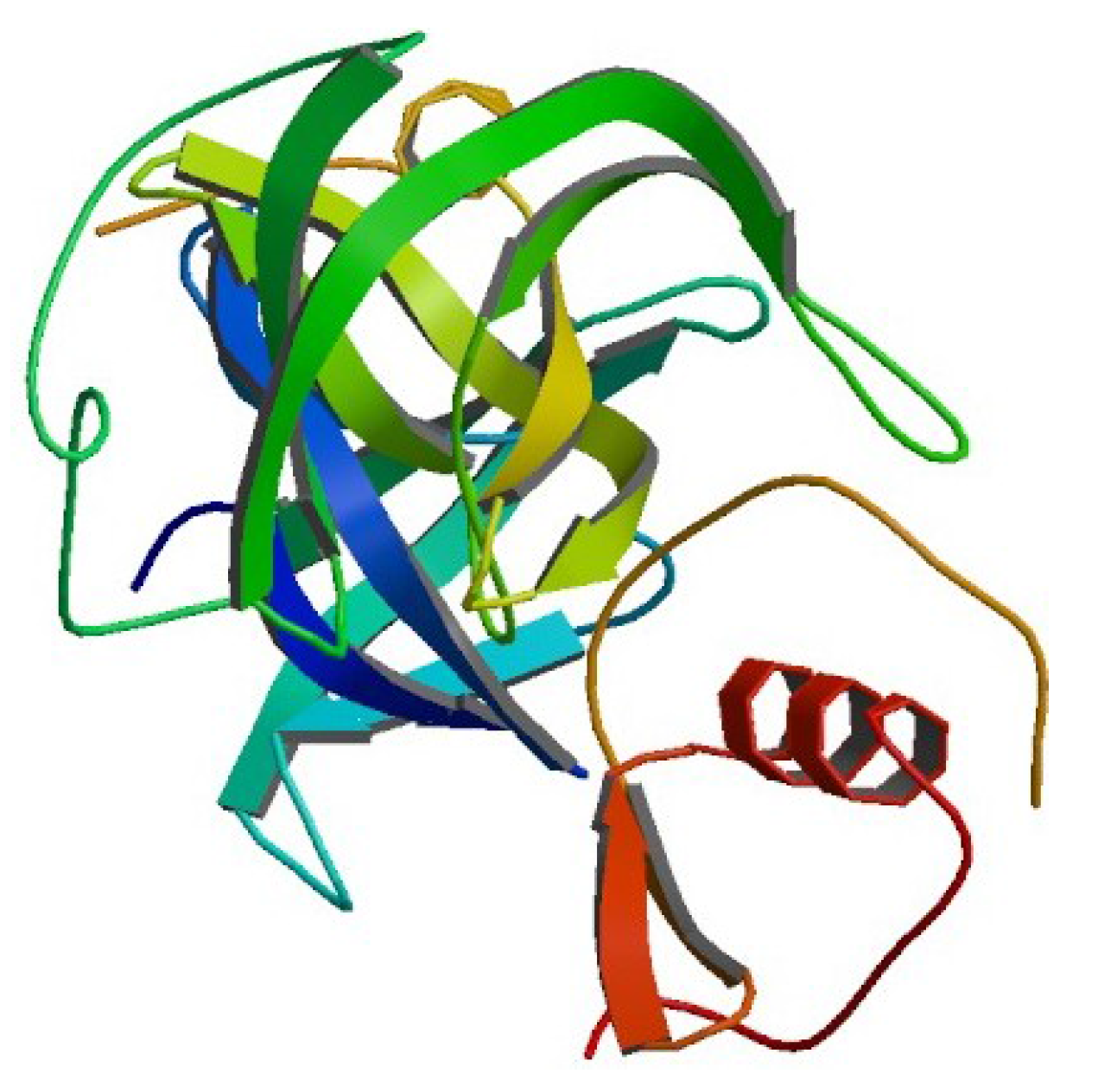
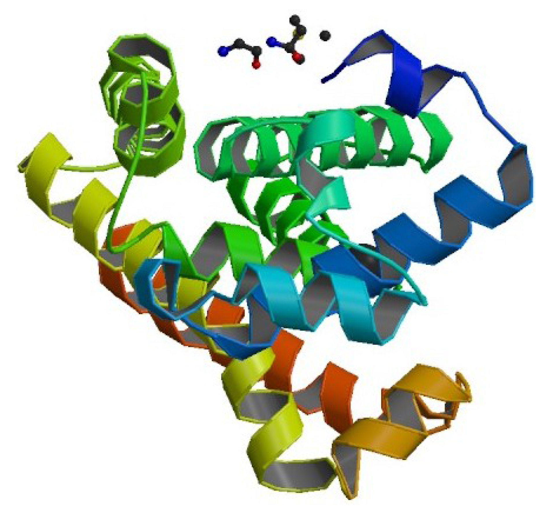
In order to contrast the proposed metrics in Section 3 with those that are purely geometric based, we perturbed a conformation given in the PDB [36] in two ways. The protein chosen is Streptomyces griseus protease B (PDB ID 3SGB) [36,38] shown in Figure 1. This protein’s loops and size make it relatively flexible and well suited to illustrate the difference between these metrics.

Figure 1. Biological assembly image of the example protein used, Streptomyces griseus protease B. Image from the RCSB PDB [39] of PDB ID 3SGB [36,38].

Figure 1. Biological assembly image of the example protein used, Streptomyces griseus protease B. Image from the RCSB PDB [39] of PDB ID 3SGB [36,38].

The perturbations are performed using a unit length vector, $\mathbf{V}\in {\mathbb{R}}^N$. Using $\mathbf{V}$ and the alpha carbon locations given in the PDB file, ${\mathbf{X}}_0^0$, a family of similar mean conformations were generated as

$${\mathbf{X}}_0^{\gamma }={\mathbf{X}}_0^0+\gamma \mathbf{V}$$

(25)

for scalar values of γ. This parameterization of mean conformations then provides a way to compare how the difference measures given in Section 3 vary over a range of RMSD values. Conformational ensembles were then generated using the conformational Boltzmann distribution described in Section 2.2 together with the hard constraints discussed in Section 2.1 and Appendix A.

The first set of comparisons that was performed was between two different perturbation vectors, $\mathbf{V}$. For the first vector we consider perturbations in the direction of low frequency normal modes. These mode shapes are associated with the dominant direction of motion for large conformational changes. We start by forming a coarse grain elastic network as described in Section 2.3 using the alpha carbons. Based on this elastic network, normal mode analysis was used to obtain the minimum nonzero eigenvalue and its associated unit-length eigenvector. This eigenvector is then used as the perturbation vector $\mathbf{V}$. The second type of perturbation applied was obtained by taking a random vector whose elements are drawn from a zero mean normal distribution with constant variance. This vector was then normalized to unit length. For these examples, all stiffness matrices were constructed using $r_0=8$ Å, $k=1$, and $\beta =1$.

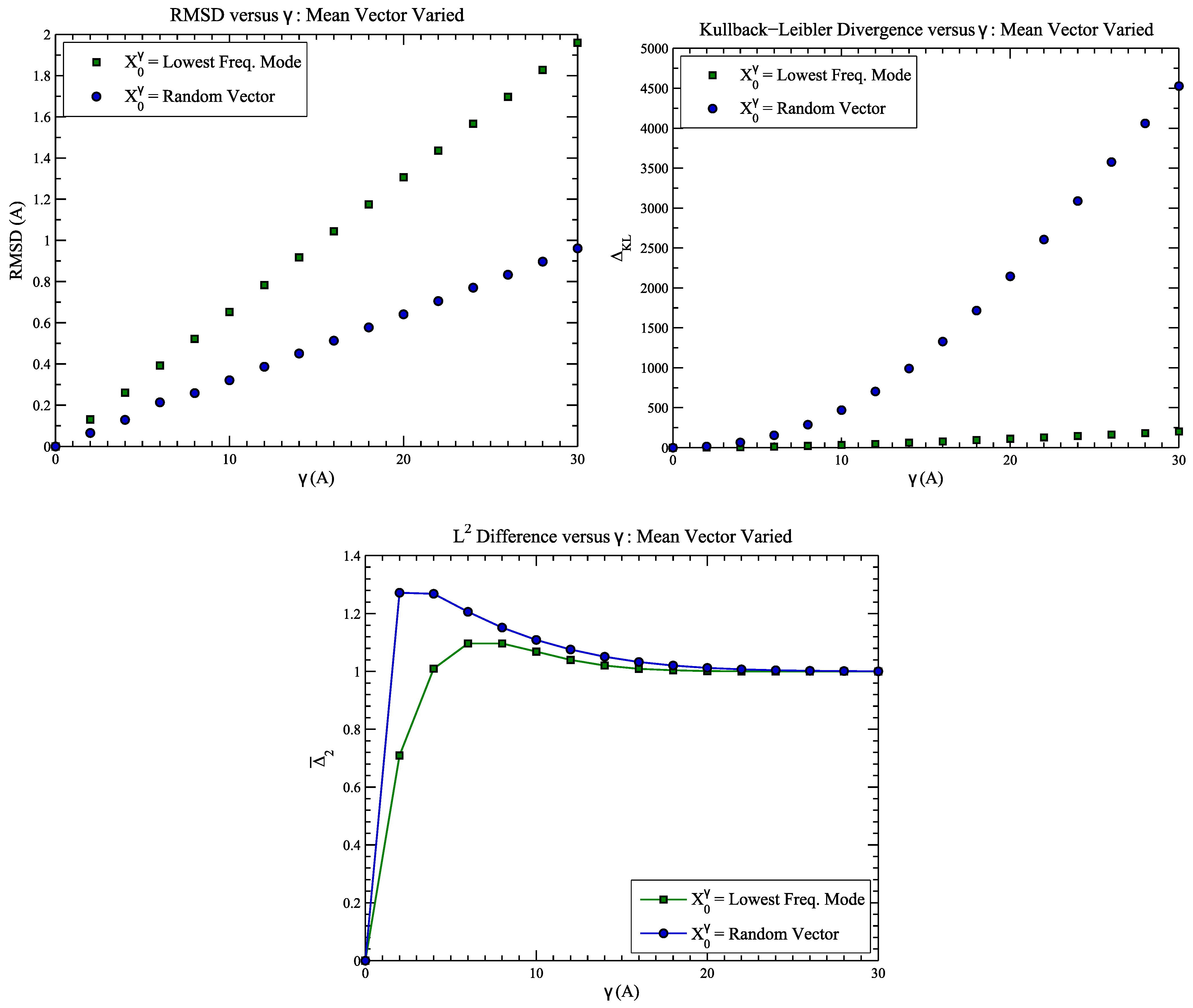
Figure 2 highlights the difference of these two perturbation methods. The conformations corresponding to the random perturbation exhibit lower RMSD values at all values of γ than perturbation in the likely direction of motion; for the random perturbations, the RMSD values are roughly half of those associated with the mode shape. This is particularly interesting when contrasted with the Kullback-Leibler divergences and $L^2$ differences. For these measures, the values associated with the normal mode perturbations are lower than those associated with the random perturbations. This can be attributed to the fact these deviations occur in a direction of high flexibility and both of these measures are functions of the conformation’s elastic structure. This effect is particularly pronounced for the Kullback-Leibler divergence. This result highlights the fact that RMSD alone does not capture how similar two conformations are when uncertainty is considered.

Figure 2. Here we demonstrate how RMSD (top left), Kullback-Leibler divergence (top right), and normalized $L^2$ difference (bottom) vary with γ (β and $r_0$ are fixed at 1 and 8 respectively). Two perturbation vectors are given, one corresponding to the lowest frequency mode and one random unit vector.

Figure 2. Here we demonstrate how RMSD (top left), Kullback-Leibler divergence (top right), and normalized $L^2$ difference (bottom) vary with γ (β and $r_0$ are fixed at 1 and 8 respectively). Two perturbation vectors are given, one corresponding to the lowest frequency mode and one random unit vector.

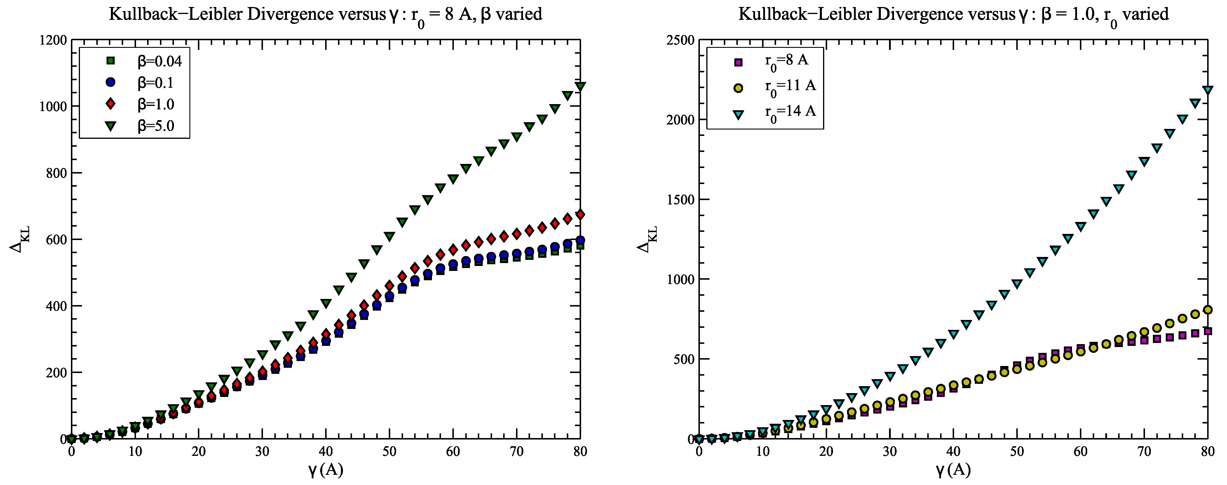
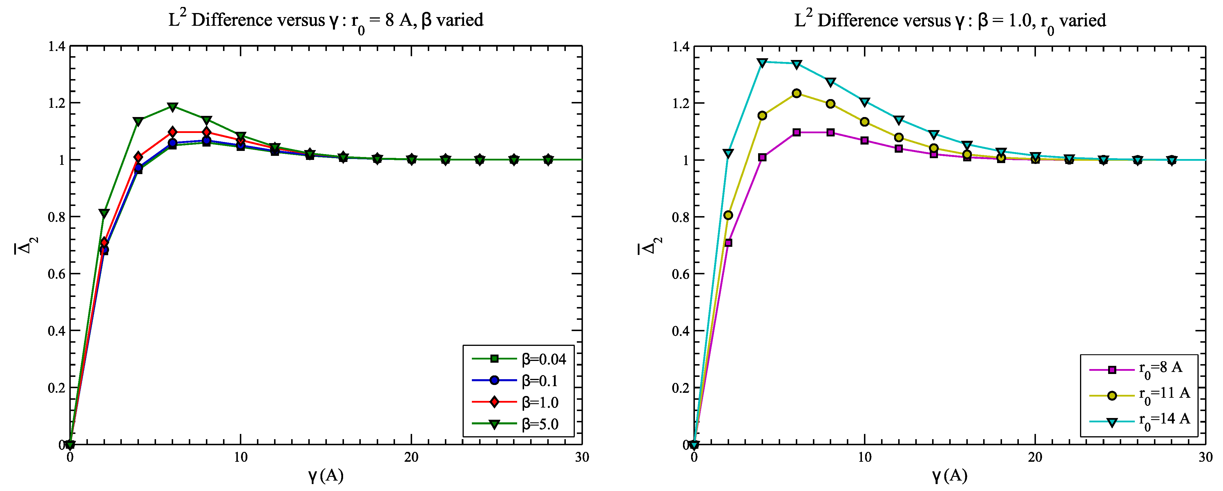
The second set of comparisons presented utilizes only the normal mode perturbation. However, a variety of values for β and $r_0$ were used as these parameters effectively alter the “stiffness” of the conformational Boltzmann distribution for a fixed value of k ($k=1$ for these examples). Figure 3 and Figure 4 demonstrate the effect of varying β and the cutoff radius, $r_0$. It should be noted that the wide range of β values being shown are only for the purpose of illustrating the relative sensitivity of our results to β. The values used may not represent a physiologically realizable range.

Figure 3. These plots illustrate how Kullback-Leibler divergence, ${\Delta }_{KL}(f_c(\tilde{\mathbf{X}},{\tilde{\mathbf{X}}}_0^0,\beta )\parallel$ $f_c(\tilde{\mathbf{X}},{\tilde{\mathbf{X}}}_0^{\gamma },\beta ))$ varies with γ for several values of β (left) and several values of $r_0$ (right).

Figure 3. These plots illustrate how Kullback-Leibler divergence, ${\Delta }_{KL}(f_c(\tilde{\mathbf{X}},{\tilde{\mathbf{X}}}_0^0,\beta )\parallel$ $f_c(\tilde{\mathbf{X}},{\tilde{\mathbf{X}}}_0^{\gamma },\beta ))$ varies with γ for several values of β (left) and several values of $r_0$ (right).

Figure 4. These plots illustrate how normalized $L^2$ difference, ${\overline{\Delta }}_2(f_c(\tilde{\mathbf{X}},{\tilde{\mathbf{X}}}_0^0,\beta )$, $f_c(\tilde{\mathbf{X}},{\tilde{\mathbf{X}}}_0^{\gamma },\beta ))$ varies with γ for several values of β (left) and several values of $r_0$ (right).

Figure 4. These plots illustrate how normalized $L^2$ difference, ${\overline{\Delta }}_2(f_c(\tilde{\mathbf{X}},{\tilde{\mathbf{X}}}_0^0,\beta )$, $f_c(\tilde{\mathbf{X}},{\tilde{\mathbf{X}}}_0^{\gamma },\beta ))$ varies with γ for several values of β (left) and several values of $r_0$ (right).

These figures illustrate several interesting things about how these metrics differ from RMSD. The first thing to note is that while RMSD is constant with respect to β and $r_0$, both the Kullback-Leibler divergence and $L^2$ difference vary with respect to these flexibility measures. It is also apparent that ${\Delta }_{KL}$ increases with γ; although, the relationship is not linear. For “stiffer” structures (i.e., higher β or higher $r_0$), the slope of ${\Delta }_{KL}$ with respect to γ is lower and begins to flatten sooner. The relationship between ${\overline{\Delta }}_2$ and γ is more complex. Close to $\gamma =0$, ${\overline{\Delta }}_2$ increases with γ until it reaches a maximum and then begins to decline until it levels out at a value of one.

4.2. Example 2: CASP Predictions

One of the motivations for looking at metrics for conformational ensembles is for comparison of protein predictions to experimentally solved proteins. Here we present a target protein structure, T0575 from CASP9 [37] (PDB ID 3NRG [40]), and several groups’ predictions. Figure 5 provides a ribbon diagram for the target protein. We examined the 44 predictions of the target that met the following conditions: (1) the prediction contains all of the residues; (2) the prediction is a group’s “first” model (i.e., it is the model with which a group is most confident); and (3) the RMSD between the alpha carbons of the prediction and target is less than 6 Å. For each of the predictions and the target, ensembles were generated using the conformational Boltzmann distribution for $\beta =1$ and $r_0=8$ Å. Using these ensembles, the Kullback-Leibler divergence ${\Delta }_{KL}$ was determined. Figure 6 presents these values of Kullback-Leibler divergence versus their associated RMSD.

Figure 5. Biological assembly image of the protein target used, a TetR family transcriptional regulator (Caur_2714) from Chloroflexus aurantiacuss. Image from the RCSB PDB [39] of PDB ID 3NRG [36,40].

Figure 5. Biological assembly image of the protein target used, a TetR family transcriptional regulator (Caur_2714) from Chloroflexus aurantiacuss. Image from the RCSB PDB [39] of PDB ID 3NRG [36,40].

It is believed that the Kullback-Leibler divergence in this context provides an indication of how similar two conformations are in terms of topology and flexibility. To demonstrate this, we used normal mode analysis to perturb the predicted models; we added a weighted sum of the first few nonzero normal modes to the predicted models to minimize the RMSD between the prediction and the target. These first few nonzero normal modes represent the primary directions of motion for elastic networks. Let the vectors associated with the normal modes be ordered such that ${\mathbf{V}}_i$ represents the $i^{th}$ nonzero normal mode. Then we can represent this minimization over m normal modes with the following perturbed model vector similar to what was done in Equation (25)

$${\mathbf{X}}_0^{\gamma }={\mathbf{X}}_0^0+\sum _{i=1}^m{\gamma }_i{\mathbf{V}}_i$$

(26)

where ${\mathbf{X}}_0^0$ is a vector of the original coordinates of the predicted model and ${\gamma }_i$’s are scalar weights. If ${\mathbf{X}}_0^{Target}$ is the coordinate vector associated with the target structure, we can then use a cyclic gradient descent to minimize RMSD,

$$\underset{{\gamma }_i}{min}{d}_2({\mathbf{X}}_0^{Target},{\mathbf{X}}_0^{\gamma })$$

(27)

The results for this analysis can found in Figure 6 and Figure 7 for the first three normal modes ($m=3$). Figure 6 shows the original Kullback-Leibler divergence versus both the original RMSD and the RMSD optimized using the first three normal modes. Figure 7 provides the percent reduction in RMSD versus the original Kullback-Leibler divergence. In this analysis, we would expect to see the amount of minimization decrease as the Kullback-Leibler divergence increases. This trend is apparent, although there are a few outliers. We note that similar results were observed for other CASP9 targets and different values of m.

Figure 6. The Kullback-Leibler divergences between predicted models and the CASP9 target are shown with respect to RMSD. RMSDs are given for the original predictions and predictions perturbed along the first three normal modes.

Figure 6. The Kullback-Leibler divergences between predicted models and the CASP9 target are shown with respect to RMSD. RMSDs are given for the original predictions and predictions perturbed along the first three normal modes.

Figure 7. The reduction in RMSD realized by minimizing along the first three normal modes is given with respect to the Kullback-Leibler divergence between the predicted model and the target (T0575).

Figure 7. The reduction in RMSD realized by minimizing along the first three normal modes is given with respect to the Kullback-Leibler divergence between the predicted model and the target (T0575).

5. Conclusions

Measures to quantify how similar two conformational ensembles are have been articulated here. In contrast to well-known measures of shape similarity between two conformations, which are purely geometric, the comparison of ensembles here requires concepts from probability and information theory. We have illustrated how using the stiffness information in conformational ensembles for two macromolecules can be used to develop difference measures that take into account the positional uncertainty of flexible regions. These new measures are based on the Kullback-Leibler divergence and $L^2$ difference.

Numerical examples of how these measures compare with the traditional RMSD were presented. The conformational ensembles for these examples were based on coarse-grained elastic networks. It has been demonstrated that for two different conformations, the RMSD of each of them with respect to a third may not provide enough information to determine which of the conformations is more similar to the third in terms of their positional uncertainty.

The measures presented provide additional information with respect to positional uncertainty. They have the potential to be extended or combined with each other, additional information theoretic measures, and/or traditional geometric measures to make them more robust to a variety of parameters. Additionally, methods for comparing the similarity of an individual structure and an ensemble can be explored.

References and Notes

1. Holm, L.; Sander, C. Protein structure comparison by alignment of distance matrices. J. Mol. Biol. 1993, 233, 123–138. [Google Scholar] [CrossRef] [PubMed]
2. Mitchell, E.M.; Artymiuk, P.J.; Rice, D.W.; Willett, P. Use of techniques derived from graph theory to compare secondary structure motifs in proteins. J. Mol. Biol. 1989, 212, 151–166. [Google Scholar] [CrossRef]
3. Zemla, A.; Venclovas, C.; Moult, J.; Fidelis, K. Processing and analysis of CASP3 protein structure predictions. Protein. Struct. Funct. Bioinform. 1999, 37, 22–29. [Google Scholar] [CrossRef]
4. Gong, H.P.; Rose, G.D. Does secondary structure determine tertiary structure in proteins? Protein. Struct. Funct. Bioinform. 2005, 61, 338–343. [Google Scholar] [CrossRef] [PubMed]
5. Irving, J.A.; Whisstock, J.C.; Lesk, A.M. Protein structural alignments and functional genomics. Proteins 2001, 42, 378–382. [Google Scholar] [CrossRef]
6. Jewett, A.I.; Huang, C.C.; Ferrin, T.E. MINRMS: An efficient algorithm for determining protein structure similarity using root-mean-squared-distance. Bioinformatics 2003, 19, 625–634. [Google Scholar] [CrossRef] [PubMed]
7. Hilser, V.J.; Garcia-Moreno, E.B.; Oas, T. G; Kapp, G.; Whitten, S.T. A statistical thermodynamic model of the protein ensemble. Chem. Rev. 2006, 106, 1545–1558. [Google Scholar] [CrossRef] [PubMed]
8. Hilser, V.J.; Dowdy, D.; Oas, T.G.; Freire, E. The structural distribution of cooperative interactions in proteins: Analysis of the native state ensemble. Proc. Nat. Acad. Sci. U. S. A. 1998, 95, 9903–9908. [Google Scholar] [CrossRef]
9. Tyka, M.D.; Keedy, D.A.; Andre, I.; Dimaio, F.; Song, Y.; Richardson, D.C.; Richardson, J.S.; Baker, D. Alternate states of proteins revealed by detailed energy landscape mapping. J. Struct. Biol. 2011, 405, 607–618. [Google Scholar] [CrossRef] [PubMed]
10. Burra, P.V.; Zhang, Y.; Godzik, A.; Stec, B. Global distribution of conformational states derived from redundant models in the PDB points to non-uniqueness of the protein structure. Proc. Nat. Acad. Sci. U. S. A. 2009, 106, 10505–10510. [Google Scholar] [CrossRef] [PubMed]
11. Chirikjian, G.S. Modeling loop entropy. Methods Enzymol. 2011, 487, 99–132. [Google Scholar] [PubMed]
12. Zhou, H.-X. Loops in proteins can be modeled as worm-like chains. J. Phys. Chem. B 2001, 105, 6763–6766. [Google Scholar] [CrossRef]
13. Zhang, J.; Lin, M.; Chen, R.; Wang, W.; Liang, J. Discrete state model and accurate estimation of loop entropy of RNA secondary structures. J. Chem. Phys. 2008, 128. [Google Scholar] [CrossRef] [PubMed]
14. Shehu, A.; Clementi, C.; Kavraki, L.E. Modeling protein conformational ensembles: From missing loops to equilibrium fluctuations. Protein. Struct. Funct. Bioinform. 2006, 65, 164–179. [Google Scholar] [CrossRef] [PubMed]
15. Shehu, A.; Kavraki, L.E.; Clementi, C. On the characterization of protein native state ensembles. Biophys. J. 2007, 92, 1503–1511. [Google Scholar] [CrossRef] [PubMed]
16. Wu, X.; Brooks, B.R. Toward canonical ensemble distribution from self-guided Langevin dynamics simulation. J. Chem. Phys. 2011, 134, 134108:1–134108:12. [Google Scholar] [CrossRef] [PubMed]
17. Grosberg, A.Y.; Khokhlov, A.R. Statistical Physics of Macromolecules; American Institute of Physics: New York, NY, USA, 1994. [Google Scholar]
18. Jacobs, D.J.; Rader, A.J.; Kuhn, L.A.; Thorpe, M.F. Protein flexibility predictions using graph theory. Protein. Struct. Funct. Bioinform. 2001, 44, 150–165. [Google Scholar] [CrossRef] [PubMed]
19. Damm, K.L.; Carlson, H.A. Gaussian-weighted RMSD superposition of proteins: A structural comparison for flexible proteins and predicted protein structures. Biophys. J. 2006, 90, 4558–4573. [Google Scholar] [CrossRef] [PubMed]
20. Moult, J.; Pederson, J.T.; Judson, R.; Fidelis, K. A large-scale experiment to assess protein structure prediction methods. Protein. Struct. Funct. Genet. 1995, 23, ii–iv. [Google Scholar] [CrossRef] [PubMed]
21. Moult, J.; Fidelis, K.; Kryshtafovych, A.; Tramontano, A. Critical assessment of methods of protein structure prediction (CASP)—Round IX. Protein. Struct. Funct. Bioinform. 2011, 79, 1–5. [Google Scholar] [CrossRef] [PubMed]
22. Wodak, S.J. From the Mediterranean coast to the shores of Lake Ontario: CAPRI’s premiere on the American continent. Protein. Struct. Funct. Bioinform. 2007, 69, 697–698. [Google Scholar] [CrossRef] [PubMed]
23. Janin, J. Welcome to CAPRI: A critical assessment of predicted interactions. Protein. Struct. Funct. Bioinform. 2002, 47. [Google Scholar] [CrossRef]
24. Here the word “similarity” is not used in the sense of basic geometry which involves rigid-body and scale transformations, but rather describes small differences in shape.
25. Chiang, C.-J.; Chirikjian, G.S. Similarity metrics with applications in modular robot motion planning. Auton. Robot. 2001, 10, 91–106. [Google Scholar] [CrossRef]
26. Pamecha, A.; Ebert-Uphoff, I.; Chirikjian, G.S. Useful metrics for modular robot motion planning. IEEE Trans. Robot. Autom. 1997, 13, 531–545. [Google Scholar] [CrossRef]
27. The interpretation of the “action” · depends on the context. We can talk about the action on a function, g·ρ′, or on a vector, g·x, or other objects.
28. Chennubhotla, C.; Rader, A.J.; Yang, L.-W.; Bahar, I. Elastic network models for understanding biomolecular machinery: From enzymes to supramolecular assemblies. Phys. Biol. 2005, 2, 173–180. [Google Scholar] [CrossRef] [PubMed]
29. Kim, M.K.; Chirikjian, G.S.; Jernigan, R.L. Elastic models of conformational transitions in macromolecules. J. Mol. Graph. Model. 2002, 21, 151–160. [Google Scholar] [CrossRef]
30. Zheng, W.; Brooks, B.R.; Hummer, G. Protein conformational transitions explored by mixed elastic network models. Protein. Struct. Funct. Bioinform. 2007, 69, 43–57. [Google Scholar] [CrossRef] [PubMed]
31. Maragakis, P.; Karplus, M. Large amplitude conformational change in proteins explored with a plastic network model: Adenylate kinase. J. Mol. Biol. 2005, 352, 807–822. [Google Scholar] [CrossRef] [PubMed]
32. Atilgan, A.R.; Durell, S.R.; Jernigan, R.L.; Demirel, M.C.; Keskin, O.; Bahar, I. Anisotropy of fluctuation dynamics of proteins with an elastic network model. Biophys. J. 2001, 80, 505–515. [Google Scholar] [CrossRef]
33. Bahar, I.; Atilgan, A.R.; Erman, B. Direct evaluation of thermal fluctuations in proteins using a single-parameter harmonic potential. Fold. Design 1997, 2, 173–181. [Google Scholar] [CrossRef]
34. Doruker, P.; Jernigan, R.L.; Bahar, I. Dynamics of large proteins through hierarchical levels of coarse-grained structures. J. Comput. Chem. 2002, 23, 119–127. [Google Scholar] [CrossRef] [PubMed]
35. Wang, Y.; Rader, A.J.; Bahar, I.; Jernigan, R.L. Global ribosome motions revealed with elastic network model. J. Struct. Biol. 2004, 147, 302–314. [Google Scholar] [CrossRef] [PubMed]
36. Berman, H.M.; Westbrook, J.; Feng, Z.; Gilliland, G.; Bhat, T.N.; Weissig, H.; Shindyalov, I.N.; Bourne, P.E. The protein data bank. Nucleic Acids Res. 2000, 28, 235–242. [Google Scholar] [CrossRef] [PubMed]
37. CASP9. Protein Structure Prediction Center, University of California, Davis. 2010. Available online: http://predictioncenter.org/casp9/ (accessed on 25 January 2012).
38. Read, R.J.; Fujinaga, M.; Sielecki, A.R.; James, M.N. Structure of the complex of Streptomyces griseus protease B and the third domain of the turkey ovomucoid inhibitor at 1.8-A resolution. Biochemistry 1983, 22, 4420–4433, PDB ID: 3GSB. [Google Scholar] [CrossRef] [PubMed]
39. RCSB Protein Data Bank. Available online: http://www.pdb.org (accessed on 20 January 2012).
40. Joint Center for Structural Genomics. Crystal structure of a TetR family transcriptional regulator (Caur_2714) from Chloroflexus aurantiacus J-10-FL at 2.56 A resolution. PDB ID: 3NRG.
Appendix
A. Restricting the Conformational Boltzmann Distribution and Applying a Rigid-Body Transformation
Recall from Section 2.1 that we can remove 6 degrees of freedom by forcing x n 0 = 0 , rotating the conformation so that the vector from x n 0 to x n 1 0 is aligned with e 1 , and confining x n 2 0 to the plane spanned by e 1 and e 2 . The resulting coordinate vector X R 3 n can then be written as
X = x 1 x 2 x n 3 x n 2 x n 1 x n = x 1 x 2 x n 3 a 1 e 1 + a 2 e 2 a 3 e 1 0 = x 1 x 2 x n 3 a 1 a 2 0 a 3 0 0 0
Let us define B as
B = I ( 3 n 7 ) 0 0 0 0 0 0 0 0 T 0 1 0 0 0 0 0
Here B R ( 3 n 6 ) × 3 n . Let us also define
X 1 , n 3 = x 1 x 2 x n 3
The generalized coordinate system X ˜ R 3 n 6 is then
X ˜ = x 1 x 2 x n 3 a 1 a 2 a 3 = X 1 , n 3 a 1 a 2 a 3 = B X
Here, and henceforth, a 1 will represent the signed distance of x n 1 from the plane spanned by the global e 2 and e 3 axes as measured along the vector from x n 0 to x n 1 0 . This ensures that the confined degrees of freedom are respected. Also, a 2 ( a 3 ) will represent the signed distance of x n 2 from the plane spanned by the fixed global e 2 and e 3 ( e 1 and e 3 ) axes as measured along the transformed e 1 ( e 2 ) axis.
If we apply an arbitrary rigid body motion g 0 to the conformation where
g 0 = R 0 t 0 0 T 1
then
y i = R 0 x i + t 0
We can then write
R ˜ 0 = R 0 R 0 R 0
and
t ˜ 0 = t 0 t 0 t 0
where R ˜ 0 R 3 n × 3 n and t ˜ 0 R 3 n . (Note: We will let R ˜ 0 n 3 R 3 ( n 3 ) × 3 ( n 3 ) represent a direct sum of n 3 copies of R 0 .) Then the new coordinate vector can be written as
Y = R ˜ 0 X + t ˜ 0
If K X 0 is the stiffness matrix associated with X , the new stiffness matrix K Y 0 can be written as
K Y 0 = R ˜ 0 K X 0 R ˜ 0 T
Also, the stiffness matrix corresponding to X ˜ can then be written as
K ˜ X 0 = B K X 0 B T
However, in the new coordinate system that has been transformed via g 0 , a similar equality does not hold in general,
K ˜ Y 0 B K Y 0 B T
Yet there is something that can be said if we consider the rotation and translation separately. First we will consider pure translation (i.e., R 0 = I 3 );
Y = X + t ˜ 0 , Y ˜ = B Y = X ˜ + B t ˜ 0 , and K Y 0 = K X 0
Also,
K ˜ Y 0 = B K Y 0 B T = B K X 0 B T
Next, consider pure rotation (i.e., t 0 = 0 );
Y = R ˜ 0 X and K Y 0 = R ˜ 0 K X 0 R ˜ 0 T
However
Y ˜ = R ˜ 0 n 3 X 1 , n 3 a 1 a 2 a 3 = Y 1 , n 3 a 1 a 2 a 3
We can recover Y using A = I I I R 0 R 0 R 3 n × 3 n via
Y = A B T Y 1 , n 3 a 1 a 2 a 3 = A B T Y ˜
Then one can write
( Y Y 0 ) T K Y 0 ( Y Y 0 ) = ( Y ˜ Y ˜ 0 ) T B A T K Y 0 A B T ( Y ˜ Y ˜ 0 )
Therefore, for pure rotation
K ˜ Y 0 = B A T K Y 0 A B T
Using these two cases, we can generate any rigid body motion of one conformation relative to another. For example, if we want the coordinate frames attached to two conformations ( X 0 and X 0 ) to be separated by g 0 = ( R 0 , t 0 ) , we could apply g R 0 = ( R 0 , 0 ) to X 0 and g t 0 = ( I , t 0 ) to X 0 .