Entropic Approach to Multiscale Clustering Analysis

1
School of Computer Science, University of Birmingham, Edgbaston B15 2TT Birmingham, UK
2
Dipartimento di Fisica e Astronomia, Universitá di Catania and INFN, Via S. Sofia 64, 95123 Catania, Italy
*
Author to whom correspondence should be addressed.
Entropy 2012, 14(5), 865-879; https://doi.org/10.3390/e14050865
Submission received: 20 February 2012
/
Revised: 3 May 2012
/
Accepted: 4 May 2012
/
Published: 9 May 2012
(This article belongs to the Special Issue Concepts of Entropy and Their Applications)
Abstract
:Recently, a novel method has been introduced to estimate the statistical significance of clustering in the direction distribution of objects. The method involves a multiscale procedure, based on the Kullback–Leibler divergence and the Gumbel statistics of extreme values, providing high discrimination power, even in presence of strong background isotropic contamination. It is shown that the method is: (i) semi-analytical, drastically reducing computation time; (ii) very sensitive to small, medium and large scale clustering; (iii) not biased against the null hypothesis. Applications to the physics of ultra-high energy cosmic rays, as a cosmological probe, are presented and discussed.
1. Introduction
Ultra-high energy cosmic rays (UHECR) are charged particles of extreme energy coming from the outer space. Unfortunately, such particles are also extremely rare, with a flux of 1 particle per km per century above an energy of eV.
The measure of clustering in the arrival direction distribution of UHECR is of fundamental importance in astroparticle physics, because it should shed light on the possibility of astronomy by means of charged particles. In fact, because of Liouville’s theorem, clustering can not occur because of inhomogeneous magnetic fields if it is not an intrinsic feature of the data. Thus, the presence of a clustering signal should be associated with an anisotropic distribution of either sources or their luminosity, responsible of event excesses in a privileged direction instead of another one. Moreover, when energy losses are taken into account during the propagation, as it should be, the distribution of (unknown) sources with respect to redshift plays a significant role: the existence of the Greisen–Zatsepin–Kuzmin [1,2] effect should drastically reduce the number of candidate sources, by restricting their allowed positions to a sphere with radius of a few hundreds Mpc (1 Mpc km). Observations suggest that the distribution of candidate sources in the nearby universe, e.g., AGN or rapidly rotating neutron stars, is strongly anisotropic. Hence, in the absence of clusters of UHECR, sources are expected to be isotropically distributed and characterized by equally intrinsic luminosity.
In the last decade, many efforts have been made to detect a clustering signal in the arrival direction distribution of UHECR (see [3,4,5] and references therein), by means of the two-point angular correlation function estimating the excess of pairs with respect to the isotropic expectation as a function of the angular scale. However, only a few number of events are publicly available for clustering analysis and even a smaller number of events has been observed with high accuracy in both direction and energy [6,7,8].
We have recently proposed a new method, based on information entropy, that is able to improve the detection of the clustering signal even in small datasets of UHECR events [9]. The concept of information entropy, introduced by Shannon some decades ago [10], has drastically changed the way of investigating the real world: a revolution similar to that carried out by Boltzmann in physics more than one century ago.
Shannon entropy quantifies the expected value of information contained in a stochastic variable, measuring the uncertainty associated with such a variable. Hence, it provides an estimation of the average amount of information loss if the value of the stochastic variable is not known.
The practical applications of such a concept in any research field are uncountable. Within the present work we focus on the detection of a clustering signal in the direction distribution of objects on a spherical surface. Clustering detection in the directions of objects plays a fundamental role in many fields, e.g., in particle physics, in astrophysics and in astroparticle physics, to cite just some of them.
In the following, we will describe a novel clustering detection method [9], an entropic approach based on the Kullback–Leibler divergence and the Gumbel statistics of extremal values. Although our method applies to any distribution of objects on a spherical surface, we will present an application to the physics of UHECR. The search for clustering is able to distinguish between different astrophysical scenarios (see, for instance, [11,12] and references therein): within this work, we will show an example of how it may act as a cosmological probe, being sensitive to the value of the Hubble parameter at present time, which plays a fundamental role in the comprehension of our Universe.
2. Model Selection with the Kullback–Leibler Divergence
The statistical modeling of real data represents one of the major challenge in data analysis. The first step generally involves evaluation of the goodness-of-fit of the statistical model: hence, the choice of a suitable indicator quantifying the distance between the model and the data is of fundamental importance. Although the literature is rich of criteria to evaluate the best model, the most classical of such indicators is the distance defined by Pearson.
Another interesting indicator of such a family is the Kullback–Leibler divergence, involving the concept of information entropy, with a wide variety of applications to hypothesis testing and model selection [13,14,15], statistical mechanics [16,17,18], quantum mechanics [19,20,21,22], medical [23] and ecological [24] studies, to cite just some of them. In particular, a replica-inference method has been recently applied to unsupervised image segmentation on multiple scales, in order to identify tightly bound clusters against a background [25]. Such a method makes use of extremal information theory and it depends on a resolution parameter which can be related to the intrinsic clustering scale.
Within this paper, we assume the framework of a measurable space Υ with algebra . We indicate with the space of all probability measures on and with ζ and ρ two probability measures on Υ. Let p and q denote their corresponding density functions with respect to a finite dominating measure x. Hence, the Kullback–Leibler (KL) divergence [26,27], quantifying the error in approximating the density by means of , is defined by
where is the support of ζ on Υ. In the case of a countable measurable space the definition reduces to
The KL divergence is non-negative, i.e., with equality holding if and only if the probability distributions P and Q corresponding to p and q densities, respectively, are equal. Moreover, the KL divergence is asymmetric, i.e., . If a finite set of candidate models with probability density () is available, model selection is simply performed by estimating the corresponding set of values and selecting the model which provides the lowest value of the divergence. The statistical interpretation of KL divergence is as follows.
Let be the empirical distribution of random outcomes () of the true distribution P, putting the probability on each outcome as
and let be the statistical model for the data, depending on the unknown parameter Θ. It follows
where is the information entropy of , not depending on Θ; and are the densities corresponding to and , respectively. Putting Equation (3) in the right-hand side of Equation (4):
where is the log-likelihood of the statistical model. It directly follows that
where the function retrieves the minimum (maximum) of the function . Hence, another way to obtain the maximum likelihood estimation is to minimize the KL divergence [28]; indeed, it can be shown that the KL divergence corresponds to the expected log-likelihood ratio [29]. Another interesting application relates the KL divergence to the standard distance , by
here reported for the sake of completeness (see [30] and references therein for further detail).
The KL divergence play a fundamental role in the method we have developed to perform clustering analysis on the directions of objects on a spherical surface, as we will see further in the text.
3. Extreme Value Statistics
Extreme value statistics, together with the KL divergence, represent the other fundamental ingredient required by our method for the detection of a clustering signal.
Extreme value theory is the research area dealing with the statistical analysis of the extremal values of a stochastic variable. Let () be i.i.d. random outcomes of a probability distribution F. If , the probability to obtain an outcome greater or equal than is:
It can be shown that the limiting distribution is degenerate and should be normalized [31]. However, if it is possible to find sequences of real constants and such that
then
The function is the generalized extreme value (GEV) distribution, also known as Fisher–Tippett function, defined by
defined for if and for if . The quantities and ξ indicate the location, scale and shape parameters, respectively. One of the Gumbel distributions, of particular interest for the present study, is related to the distribution of maxima [32,33] and it is retrieved for [31]. The corresponding probability density is easily obtained from the Fisher–Tippet distribution as
It is worth noticing that the two parameters μ and σ can be related to the mean and to the standard deviation of the distribution, by means of the following relations:
where is the Euler constant.
4. The Multiscale Autocorrelation Function
Within this section, we describe our method for the detection of a clustering signal, based on both model selection by means of the KL divergence and hypothesis testing by means of extreme value statistics [9]. The method is rather general and applies to any distribution of angular coordinates on the sphere: in the following, we consider the simplest case of testing against the hypothesis of an underlying isotropic distribution, of interest for several applications, although the application to any other null model(s) follows the same procedure.
Let be a region of a spherical surface and let () be a set of points locating n directions on . We name such a region a sky, because of the astrophysical application presented further in the text, but it is worth remarking that our choice is only motivated by the considered application rather than an intrinsic feature of the method. The sky is partitioned within a grid of N equal-area (and almost-equal shape) disjoint boxes () as described in [34]. Let Ω be the solid angle covered by , whereas each box covers the solid angle
where is the apex angle of a cone covering the same solid angle: and Ω are deeply related quantities that define a scale.
Let be the fraction of points in the data set falling into the box and let be the statistical model adopted to describe the data. In our specific case, represents the expected fraction of points isotropically distributed on falling into the box . The deviation of data from the model at the scale Θ is estimated by means of the KL divergence
because of the countable number of boxes. It is straightforward to show that is minimum for an isotropic distribution of points, or, in general, when , i.e., if the statistical model is correct.
If and refer, respectively, to the data and to an isotropic realization with the same number of events, the multiscale autocorrelation function (MAF) is defined by
where and are the sample mean and the sample standard deviation, respectively, estimated from several isotropic realizations of the data. If denotes the null hypothesis of an underlying isotropic distribution for the data, the chance probability at the angular scale Θ, properly penalized because of the scan on Θ, is the probability
obtained from the fraction of null models giving a multiscale autocorrelation, at any angular scale in the parameter space , greater than or equal to that of data at the scale Θ. The null hypothesis is eventually rejected, in favor of the alternative , with probability at the angular scale Θ.
It has been shown that independently on the value of the angular scale Θ and on the number of events on , the estimator follows a half-Gaussian distribution if the null hypothesis is true [9].
The simplest definition of the counting algorithm, as shortly described above, involves the fixed grid introduced in [34], where each box only embodies the relative number of events falling in it. Unfortunately, such a static counting approach could not reveal efficiently an existing cluster. Indeed, the fixed grid may cut a cluster of points within one or more edges, causing a further loss of information at the angular scale under investigation. To overcome this possible loss of information, a type of smoothing of the grid is applied to the direction of all objects: such an approach, called dynamical counting, has been introduced in [9], where the particular application to the physics of UHECRs has been treated with some detail.
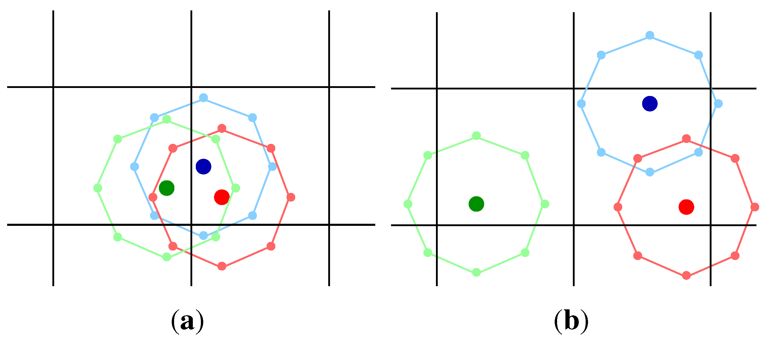
Given an angular scale Θ, we consider a set of 8 new points lying on a virtual box centered on each direction : the angular distance between each of the 8 points and the original one is constrained to be . A sketch of such a procedure is shown in Figure 1, in the case of a clustered (Figure 1a) and an unclustered (Figure 1b) set of three objects. Therefore, to each new extended point is assigned a weight, according to the characteristic of the spherical region: if all directions are equally likely, a weight equal to is assigned to the 8 extended points and the original one. (It is worth noticing that for some applications, as the case of UHECR physics, the ground-based experiments observe the sky with a non-uniform exposure, and the weight assigned to each extended point depends on its direction.)
Figure 1.
(a) Three clustered points: the extended points are mainly concentrated in two adjacent boxes; (b) Three unclustered points: the extended points are mainly distributed on the neighbor cells. (Adapted from [9], reprinted with permission from IOP Publishing, Figure 1).

Finally, we follow the procedure previously described, by using the weighted distribution of points instead of the original one. Numerical studies show that such a dynamical counting approach recovers the correct information on the amount of clustering in the data [9]. In fact, the main difference between the static and the dynamical counting lies in the value of the estimator when the procedure is applied to random realizations of the sky following the null hypothesis. For instance, the static counting is not able to recover the differences between the two configurations shown in Figure 1. Conversely, if the dynamical counting is applied, the extended points in Figure 1a are concentrated in two adjacent boxes, while in Figure 1b they are distributed on the neighbor cells. This fundamental difference is reflected in the density function, leading to two different . Monte Carlo skies producing the same clustered configuration shown in Figure 1a, and of consequence the same weight distribution, are not frequently expected: in this case, the value of should be greater than that one estimated from the static method. The direct consequence of a greater value of the estimator is a lower chance probability and the main advantage of using the dynamical counting, instead of the static one, should be the lowest penalization of only if a clustering signal is really present. In the following, we make use of the dynamical counting for any application.
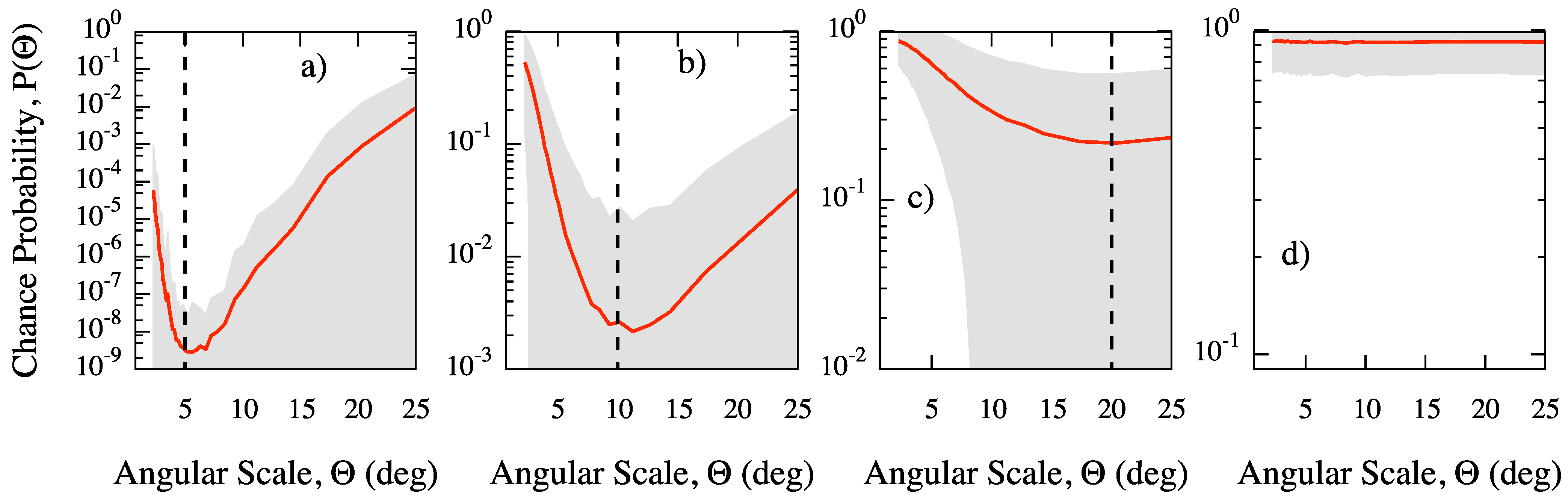
In order to illustrate the ability of our method to detect a clustering signal and the main clustering angular scale, we have generated 5000 isotropic and anisotropic skies of 100 events each on the whole sphere. In each anisotropic sky, 60% of events are normally clustered, with angular dispersion ρ, around 10 random directions, while the remaining 40% of events are isotropically distributed. For each angular scale Θ, we have estimated the chance probability for clustering. For three values of the dispersion, namely (a), (b), (c) and for the isotropic maps (d), we show in Figure 2 the average chance probability, with 68% region around the mean value, versus the angular scale. In the case of the isotropic map, the chance probability is close to one, because of the absence of clustering, and nearly flat, because all clustering scales are equally likely, as expected. Conversely, for all anisotropic maps, the average chance probability gets a minimum around the corresponding value of ρ. Thus, our estimator is able to recover the most significant clustering scale. It should be remarked that when the dispersion is used, the angular scale of the minimum is less obvious because of the large fluctuations due to the isotropic contamination and the small statistics adopted. It is worth noticing that we have observed that the curve around the value of ρ gets narrower by increasing the number of events.
Figure 2.
MAF: average chance probability (solid line), with 68% region around the mean value, estimated from isotropic and anisotropic skies generated as explained in the text. The dashed line indicates the value of the dispersion adopted to generate the corresponding mock map: (a) 5, (b) 10 and (c) 20 degrees; (d) isotropic map. (Adapted from [9], reprinted by permission from IOP Publishing, Figure 4).

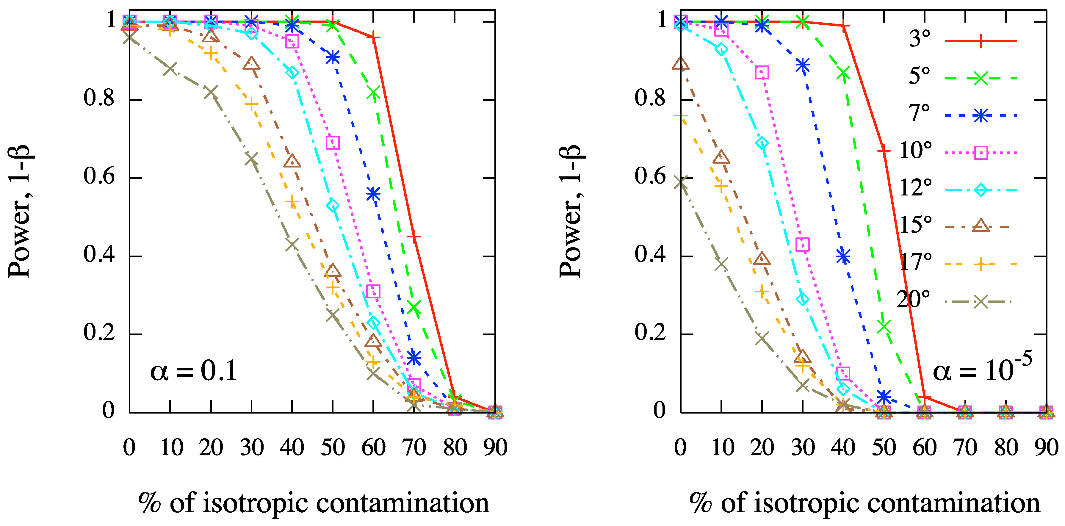
In order to further illustrate the ability of our method for clustering detection, we have considered 100 events distributed on the whole sphere, and 10 sources randomly distributed. A fixed fraction f of events are randomly clustered around the sources, while the remaining fraction of events are isotropically distributed: it follows that, on average, only events are expected around each source, further diluting the clustering signal. Hence, we have generated 1000 skies for each different value of , ranging from 0.1 to 1, and of ρ, ranging from to . Successively, we have estimated the power of the test, where β is the standard type II error rate, as a function of the isotropic fraction f, at the angular scale Θ fixed to the value chosen for ρ. In Figure 3 we show the results corresponding to fixed values of ρ, namely (left panel) and (right panel), for different values of the test significance, ranging from to . In Figure 4 we show the results corresponding to fixed values of α, namely (left panel) and (right panel), for different values of the clustering scale in simulations, ranging from to .
Figure 3.
MAF: test power as a function of the percentage of isotropic contamination in a sky of 100 events and 10 randomly distributed sources. We fix the angular scale of clustering in simulations, namely (left panel) and (right panel), and we show the test power corresponding to different values of the test significance, ranging from to , at the corresponding angular scales.

Figure 4.
As in Figure 3, but varying the angular scale of clustering in simulations from to , and fixing the test significance, namely (left panel) and (right panel).
Figure 4.
As in Figure 3, but varying the angular scale of clustering in simulations from to , and fixing the test significance, namely (left panel) and (right panel).

Even in such scenarios, where the clustering signal is strongly diluted by background contamination and distributed over different sources, the test power reveals that our method is highly efficient in clustering detection at any angular scale. In fact, for a typical value of the test significance as , the MAF is able to detect the clustering in more than 80% of cases even if the background contamination is as large as 40%–50%. Moreover, the test power decreases for increasing angular scale, as expected, although it keeps larger than 60% in scenarios with large-scale clustering (e.g., ) of 70 events out 100, in a test with significance . We remark that such a result is not trivial because of the small size of the dataset and the strong background contamination.
Relationship with extreme value statistics. Because of the definition in Equation (13) and of the central limit theorem, a Gaussian distribution is expected for the function if the null hypothesis is true, and, of consequence, the half-normal distribution
for , is expected for the estimator (normalized to zero mean and unitary variance) defined by Equation (14). Numerical studies confirm such an expectation: more intriguingly, the result does not depend either on the number of objects on the sphere or the angular scale considered [9]. It follows that the (unpenalized) probability to obtain by chance a value of the MAF, greater than or equal to a given value , is just , being erf the standard error function, independently of the angular scale Θ. Such a result allows to avoid the use of a large number of random realizations to estimate the unpenalized chance probability.
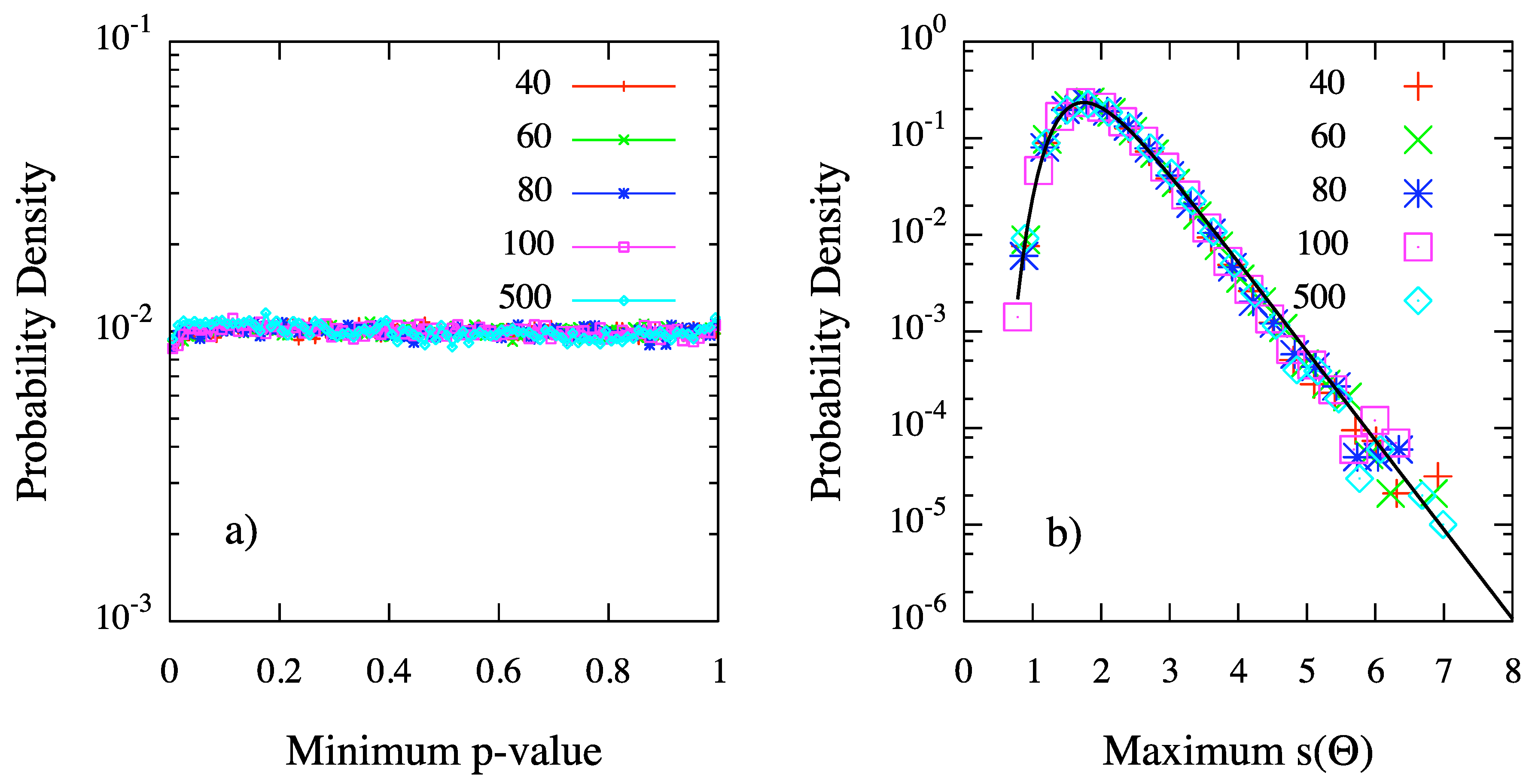
We have also verified that our method is not biased against the null hypothesis . In fact, we have generated isotropic maps of skies, by varying the number of events from 20 to 500. For each sky in each map, we have estimated the MAF for several values of the angular scale Θ. Hence, we have chosen the value of where the chance probability is minimum, as the most significant clustering scale:
properly penalized because of the scan on the parameter Θ, according to the definition in Equation (15). With no regards for the number of events in the synthetic map, we have found an excellent flat distribution of probabilities , shown in Figure 5a for skies of different size, as expected if is true. In other words, MAF is not biased against the null hypothesis, as required by suitable statistical estimators.
Despite this important feature of the MAF estimator, generally the distribution of under the null hypothesis is of interest for applications, because of the required penalization due to the scan over the parameter Θ. Intriguingly, our numerical studies show that such a distribution corresponds to the expected Gumbel function introduced in the previous section. The probability densities of for and 500 events are shown in Figure 5b: independently on n, each density is in excellent agreement with the Gumbel distribution of extreme values, with parameters and . Such values correspond to the mean and to the standard deviation of the distribution, and , respectively. It follow that the probability to obtain a maximum value of , at any angular scale Θ, greater than or equal to a given value is
providing an analytical expression for the penalized probability defined by Equation (15). Such a result is non-trivial and of great interest for practical applications: in fact, it allows to avoid the simulation of the large number of random realizations generally required to estimate the penalized probability.

5. Application to the Physics of UHECRs
The individuation of a clustering signal in the direction distribution of objects on a spherical region may be of interest for several reasons, depending on the particular problem under investigation. For instance, in [9] it has been shown the great potential of the multiscale function for clustering detection in skies of a few events and/or strongly contaminated by an isotropic background, an application of particular interest for the physics of UHECRs, generally working with small data sets. Other studies show the important role of clustering in estimating the bounds to the density of UHECR sources [11] and in probing the cosmological parameters [12].
Within the present work we show an application of clustering analysis of interest in astrophysics and cosmology. However, the treatment of the propagation of UHE protons in the Universe, propaedeutic to understand how simulations of the skies are performed, is beyond the scope of the present study, and we refer to [12] for a comprehensive description of such a topic and for further details. Here, we limit to mention that for an UHE proton generated by an astrophysical source at a certain distance z, the probability to reach the Earth with energy above a given threshold depends on its initial energy and on the redshift z. Under some assumptions regarding the injection spectrum at the source and the distribution of sources, such a probability can be estimated by means either of simulations or of an approximate analytic treatment and it is found to decrease for increasing values of z and . Moreover, is sensitive to the value of the Hubble parameter at the present time, a number of great interest in cosmology which measures the ratio of the speed of recession of a galaxy, due to the expansion of the Universe, to its distance from the observer. Hence, we explore the possibility that the estimation of the clustering signal is itself sensitive to the value of .
The simulation setup is described in detail in [12]. We consider as sources the Active Galactic Nuclei in the nearby Universe (up to ≈200 Mpc), reported in the SWIFT-BAT 58-months catalog [35]: the probability to get an event from a source is proportional to , being its intrinsic luminosity and z its distance from the Earth. The effects of intervening extragalactic magnetic fields is considered, smearing the direction around the source by sampling a Fisher–von Mises distribution, i.e., the Gaussian counterpart on the sphere. The spreading angle depends on z, on the energy of the proton and on the magnetic field considered: in our case, we consider a r.m.s. strength nG and a correlation length Mpc, according to the most recent upper bounds [36]. Protons are then propagated in a Λ-Cold Dark Matter Universe until they reach the Earth. We consider only UHECRs with energy above 100 EeV and with arrival direction lying in the field of view of the Pierre Auger Observatory, the largest observatory of UHECRs, whose non-uniform exposure is taken into account, as well as its angular uncertainty of [37]. Additionally, according to the result reported by Pierre Auger Collaboration in the case of the SWIFT-BAT 58-months catalog, the 56% of events in the simulated sky are isotropically distributed [8].
Figure 6.
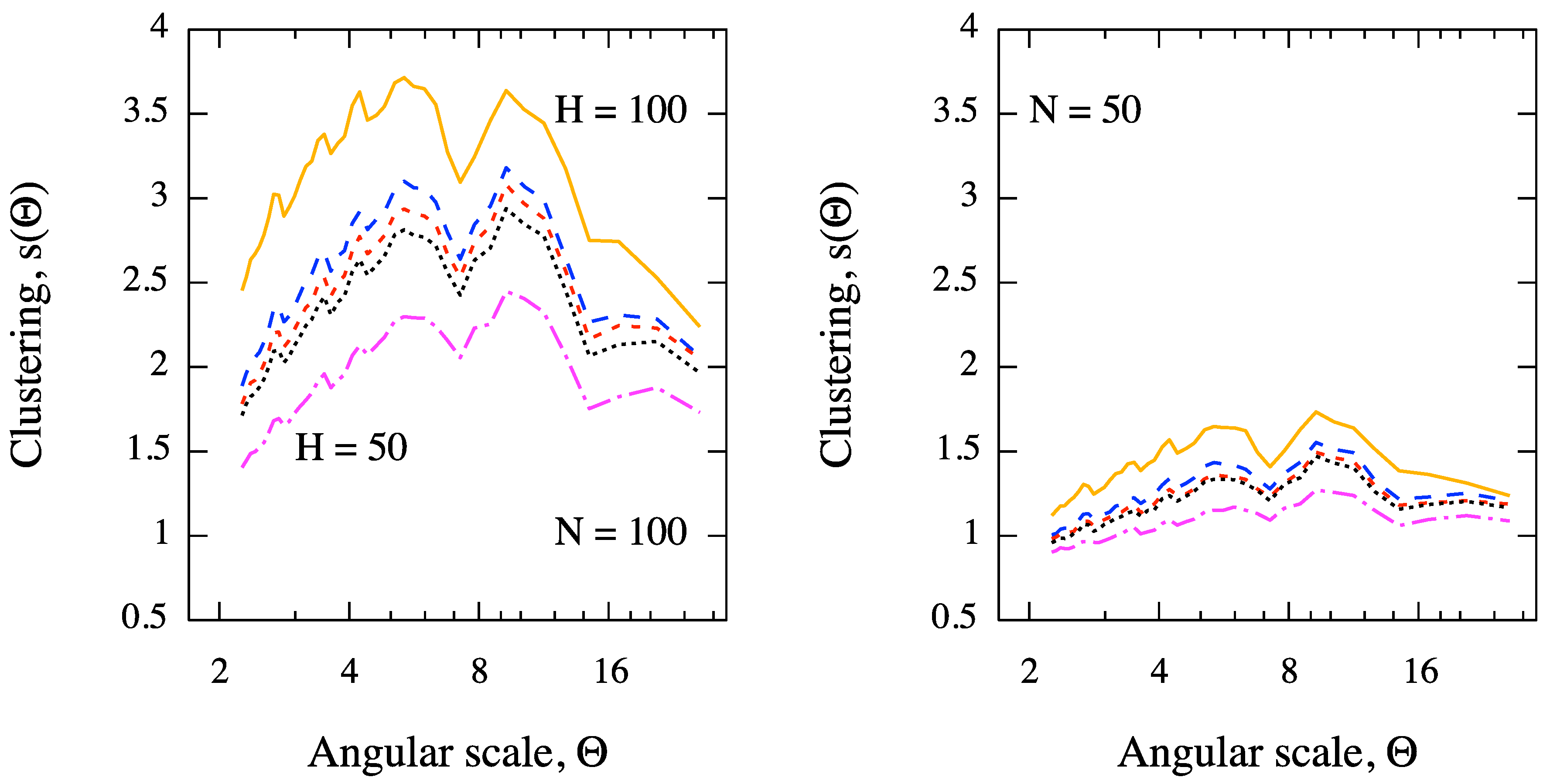
Expected clustering signal, as a function of the angular scale, from a sky of protons with EeV (in the field of view of Pierre Auger Observatory) and for values of the Hubble parameter ranging from 50 to 100 km/s/Mpc. Sources of 44% of events are AGN within 200 Mpc in the SWIFT-BAT 58-months catalog, whereas the remaining 56% of events are isotropically distributed. The intrinsic luminosity of AGN is taken into account. The clustering for (left panel) and (right panel) is considered. The signal at each angular scale is obtained by averaging over Monte Carlo realizations.
Figure 6.
Expected clustering signal, as a function of the angular scale, from a sky of protons with EeV (in the field of view of Pierre Auger Observatory) and for values of the Hubble parameter ranging from 50 to 100 km/s/Mpc. Sources of 44% of events are AGN within 200 Mpc in the SWIFT-BAT 58-months catalog, whereas the remaining 56% of events are isotropically distributed. The intrinsic luminosity of AGN is taken into account. The clustering for (left panel) and (right panel) is considered. The signal at each angular scale is obtained by averaging over Monte Carlo realizations.

We investigate the clustering signal, averaged over Monte Carlo realizations (for each astrophysical scenario corresponding to a different value of the Hubble parameter), versus the angular scale. Moreover, we vary the number of events in the sky. The results are shown in Figure 6, for different astrophysical scenarios and angular scales. It is evident that, for a fixed number of events, the clustering signal increases for increasing values of , whereas it decreases for decreasing number of events, as expected [9,12].
The astrophysical interpretation of such a result is beyond the scope of the present study. However, it is worth remarking the ability of our multiscale method to distinguish between different astrophysical scenarios even in the case of a small data set of events and a strong background contamination (56% of events are isotropically distributed). A direct comparison, as a function of the angular scale, between the clustering signal obtained from the data and that one obtained from simulations, for different values of , represents a suitable tool for probing the Hubble parameter from clustering measurements. Such a result puts in evidence the power of our entropic approach in clustering detection.
Figure 7.
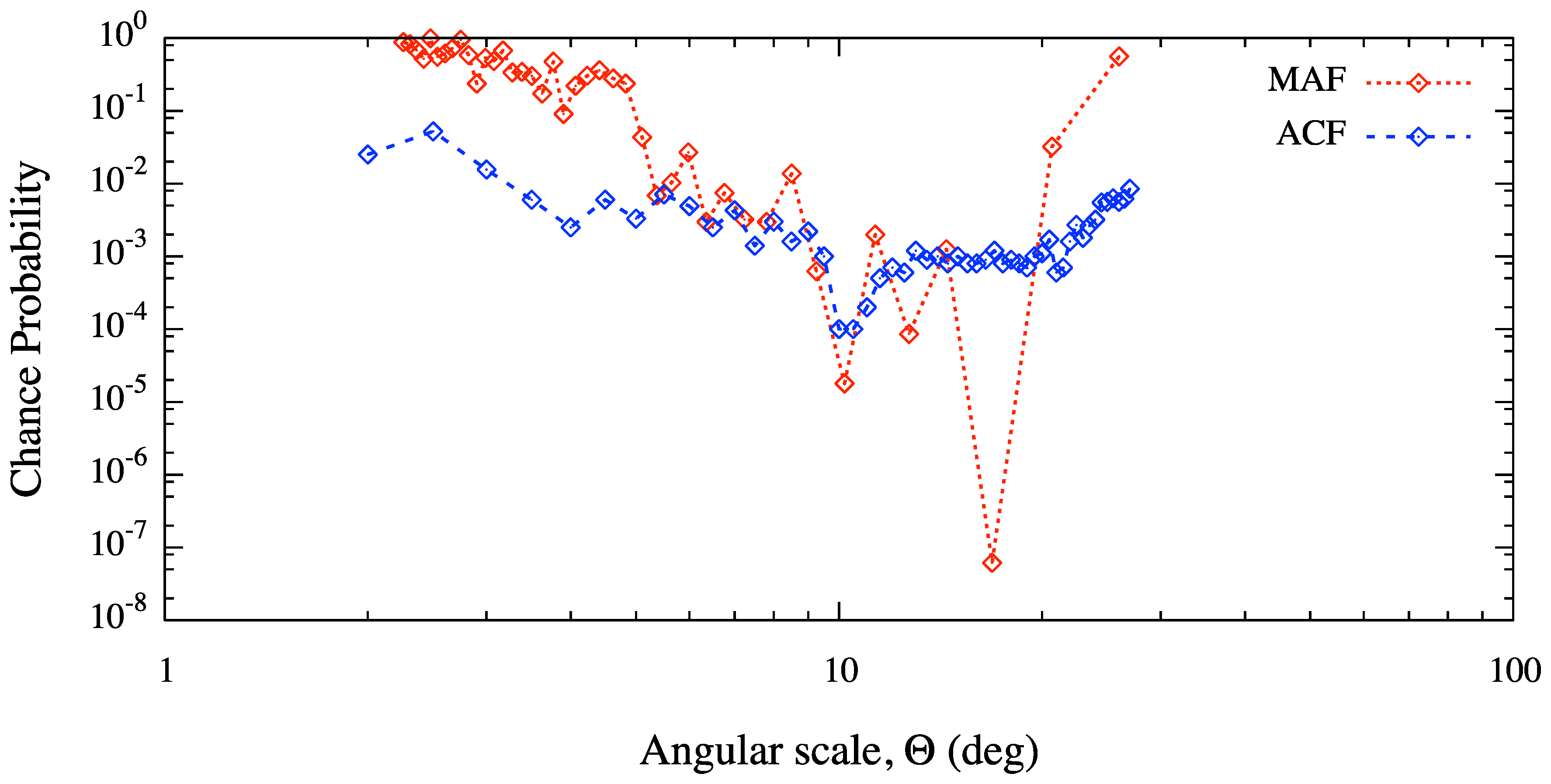
Chance probability (not penalized for the scan over Θ) for clustering as a function of the angular scale, estimated from the set of 27 UHECR events detected with the Pierre Auger Observatory. Results obtained from multiscale autocorrelation function (MAF) and two-points angular correlation function (ACF) are compared.
Figure 7.
Chance probability (not penalized for the scan over Θ) for clustering as a function of the angular scale, estimated from the set of 27 UHECR events detected with the Pierre Auger Observatory. Results obtained from multiscale autocorrelation function (MAF) and two-points angular correlation function (ACF) are compared.

Finally, we present an application on real data and we compare our result against that one obtained from the two-point angular correlation function (ACF), a standard tool adopted in clustering analysis of the arrival direction distribution of UHECR [3,4,5,6,7,8,11]. The ACF measures the cumulative number of pairs within the angular distance Θ: it is defined by
where n is the number of UHECR being considered, H is the step function and is the angular distance between events i and j. We have chosen to estimate the clustering in the arrival direction distribution of 27 UHECR events with energy above eV detected with the Pierre Auger Observatory [6,7]. The unpenalized chance probability to obtain a number of pairs greater than or equal to the data is shown in Figure 7 as a function of the angular scale Θ. For comparison, we show the result obtained with MAF from the same dataset of events. The most significant clustering scale obtained with ACF corresponds to ≈, with an unpenalized probability of ≈. The result obtained with our method is in perfect agreement with ACF, but it also suggests the existence of an even more significant clustering scale at ≈, with an unpenalized probability of ≈ and a value, properly penalized because of the scan over Θ, of ≈. Such a result is rather intriguing because of its possible astrophysical interpretations, and it puts in evidence the ability of our method in detecting the significant clustering scales in small dataset of events with respect to ACF, the most used estimator adopted for the clustering analysis of UHECR.
6. Conclusions
Within the present work, we have described a new fast and simple method for clustering detection in the direction distribution of objects on a spherical surface. The method makes use of a multiscale approach, based on the concept of information entropy and extreme value statistics, and it depends on one parameter only, namely the angular scale of the intrinsic clustering. The main advantage of our estimator is the possibility to treat the results semi-analytically: in any blind search, computation time required to statistically penalize the results is drastically reduced, allowing the possibility of applications to very large data sets of objects.
As a practical application, we have used the amount of clustering in the arrival direction distribution of ultra-high energy cosmic rays to probe the Hubble parameter at the present time. Results show that our method is suitable to detect such a clustering signal in a small dataset of events, even in presence of a strong contaminating background component. Hence, the whole procedure can be adopted as a cosmological probe.
Finally, by using a small dataset of real events, we have shown that our method provides more information about clustering than the two-point angular correlation function, the most used estimator for clustering detection in the physics of ultra-high energy cosmic rays.
References
- Greisen, K. End to the cosmic-ray spectrum? Phys. Rev. Lett. 1966, 16, 748–750. [Google Scholar] [CrossRef]
- Zatsepin, G.; Kuz’Min, V. Upper limit of the spectrum of cosmic rays. JETP Lett. 1966, 4, 78–80. [Google Scholar]
- Kachelrieß, M.; Semikoz, D. Clustering of ultra-high energy cosmic ray arrival directions on medium scales. Astropart. Phys. 2006, 26, 10–15. [Google Scholar] [CrossRef]
- Cuoco, A.; Hannestad, S.; Haugbølle, T.; Kachelrieß, M.; Serpico, P. Clustering properties of ultra-high-energy cosmic rays. Astrophys. J. 2008, 676, 807–815. [Google Scholar] [CrossRef]
- Cuoco, A.; Hannestad, S.; Haugbølle, T.; Kachelrieß, M.; Serpico, P. A global autocorrelation study after the first Auger data. Astrophys. J. 2009, 702, 825–832. [Google Scholar] [CrossRef]
- The Pierre Auger Collaboration. Correlation of the highest-energy cosmic rays with nearby extragalactic objects. Science 2007, 318, 938–943. [Google Scholar]
- The Pierre Auger Collaboration. Correlation of the highest-energy cosmic rays with the positions of nearby active galactic nuclei. Astropart. Phys. 2008, 29, 188–204. [Google Scholar]
- The Pierre Auger Collaboration. Update on the correlation of the highest energy cosmic rays with nearby extragalactic matter. Astropart. Phys. 2010, 34, 314–326. [Google Scholar] [Green Version]
- De Domenico, M.; Insolia, A.; Lyberis, H.; Scuderi, M. Multiscale autocorrelation function: A new approach to anisotropy studies. J. Cosmol. Astropart. Phys. 2011, 03. [Google Scholar] [CrossRef] [PubMed]
- Shannon, C. A mathematical theory of communication. Bell Syst. Tech. J. 1948, 27, 379–423, 623–656. [Google Scholar] [CrossRef]
- De Domenico, M.; for The Pierre Auger Collaboration. Bounds on the Density of Sources of Ultra High Energy Cosmic Rays from Pierre Auger Observatory Data. In Proceedings of the 32nd ICRC, Beijing, China, 11 August 2011.
- De Domenico, M.; Insolia, A. Influence of cosmological models on the GZK horizon of ultrahigh energy protons. arXiv 2012. [Google Scholar] [CrossRef]
- Akaike, H. Information Theory and an Extension of the Maximum Likelihood Principle. In Proceedings of the 2nd International Symposium on Information Theory, Tsahkadsor, Armenia, U.S.S.R., September 2–8, 1971; pp. 267–281.
- Akaike, H. A new look at the statistical model identification. IEEE Trans. Autom. Control 1974, 19, 716–723. [Google Scholar] [CrossRef]
- Anderson, D.; Burnham, K.; Thompson, W. Null hypothesis testing: Problems, prevalence, and an alternative. J. Wildl. Manag. 2000, 64, 912–923. [Google Scholar] [CrossRef]
- Plastino, A.; Plastino, A.; Miller, H. On the relationship between the Fisher-Frieden-Soffer arrow of time, and the behaviour of the Boltzmann and Kullback entropies. Phys. Lett. A 1997, 235, 129–134. [Google Scholar] [CrossRef]
- Plastino, A.; Miller, H.; Plastino, A. Minimum Kullback entropy approach to the Fokker-Planck equation. Phys. Rev. E 1997, 56, 3927–3934. [Google Scholar] [CrossRef]
- Portesi, M.; Pennini, F.; Plastino, A. Geometrical aspects of a generalized statistical mechanics. Physica A 2007, 373, 273–282. [Google Scholar] [CrossRef]
- Fuchs, C. Distinguishability and accessible information in quantum theory. arXiv 1995. [Google Scholar]
- Reginatto, M. Derivation of the equations of nonrelativistic quantum mechanics using the principle of minimum Fisher information. Phys. Rev. A 1998, 58, 1775–1778. [Google Scholar] [CrossRef]
- Abe, S.; Rajagopal, A. Quantum entanglement inferred by the principle of maximum nonadditive entropy. Phys. Rev. A 1999, 60, 3461–3466. [Google Scholar] [CrossRef]
- Abe, S. Nonadditive generalization of the quantum Kullback-Leibler divergence for measuring the degree of purification. Phys. Rev. A 2003, 68, 32302. [Google Scholar] [CrossRef]
- Gersch, W.; Martinelli, F.; Yonemoto, J.; Low, M.; Mc Ewan, J. Automatic classification of electroencephalograms: Kullback-Leibler nearest neighbor rules. Science 1979, 205, 193–195. [Google Scholar] [CrossRef] [PubMed]
- Burnham, K.; Anderson, D. Kullback-Leibler information as a basis for strong inference in ecological studies. Wildl. Res. 2001, 28, 111–120. [Google Scholar] [CrossRef]
- Hu, D.; Ronhovde, P.; Nussinov, Z. Replica inference approach to unsupervised multiscale image segmentation. Phys. Rev. E 2012, 85, 016101. [Google Scholar] [CrossRef]
- Kullback, S.; Leibler, R. On information and sufficiency. Ann. Math. Stat. 1951, 22, 79–86. [Google Scholar] [CrossRef]
- Kullback, S. The Kullback-Leibler distance. Am. Stat. 1987, 41, 340–341. [Google Scholar]
- Cover, T.; Thomas, J. Elements of Information Theory; Wiley Series in Telecommunications: Weinheim, Germany, 1991. [Google Scholar]
- Eguchi, S.; Copas, J. Interpreting kullback-leibler divergence with the neyman-pearson lemma. J. Multivar. Anal. 2006, 97, 2034–2040. [Google Scholar] [CrossRef]
- Sayyareh, A. A new upper bound for Kullback-Leibler divergence. Appl. Math. Sci. 2011, 5, 3303–3317. [Google Scholar]
- de Haan, L.; Ferreira, A. Extreme Value Theory: An Introduction; Springer Verlag: Berlin, Heidelberg, Germany, 2006. [Google Scholar]
- Gumbel, E. Statistical Theory of Extreme Values and Some Practical Applications: A Series of Lectures; National Bureau of Standards: Washington, DC, USA, 1954. [Google Scholar]
- Gumbel, E. Statistics of Extremes; Dover Pub.: New York, USA, 2004. [Google Scholar]
- Stokes, B.; Jui, C.; Matthews, J. Using fractal dimensionality in the search for source models of ultra-high energy cosmic rays. Astropart. Phys. 2004, 21, 95–109. [Google Scholar] [CrossRef]
- Baumgartner, W.H.; Tueller, J.; Markwardt, C.; Skinner, G. The Swift-BAT 58 Month Survey; Bulletin of the American Astronomical Society; American Astronomical Society: Washington, DC, USA, 2010; Volume 42, p. 675. [Google Scholar]
- Trivedi, P.; Subramanian, K.; Seshadri, T. Primordial magnetic field limits from cosmic microwave background bispectrum of magnetic passive scalar modes. Phys. Rev. D 2010, 82, 123006. [Google Scholar] [CrossRef]
- Bonifazi, C.; for The Pierre Auger Collaboration. The angular resolution of the Pierre Auger observatory. Nucl. Phys. B 2009, 190, 20–25. [Google Scholar] [CrossRef]
© 2012 by the authors; licensee MDPI, Basel, Switzerland. This article is an open access article distributed under the terms and conditions of the Creative Commons Attribution license (http://creativecommons.org/licenses/by/3.0/.)
Share and Cite
MDPI and ACS Style
De Domenico, M.; Insolia, A. Entropic Approach to Multiscale Clustering Analysis. Entropy 2012, 14, 865-879. https://doi.org/10.3390/e14050865
AMA Style
De Domenico M, Insolia A. Entropic Approach to Multiscale Clustering Analysis. Entropy. 2012; 14(5):865-879. https://doi.org/10.3390/e14050865
Chicago/Turabian StyleDe Domenico, Manlio, and Antonio Insolia. 2012. "Entropic Approach to Multiscale Clustering Analysis" Entropy 14, no. 5: 865-879. https://doi.org/10.3390/e14050865