Article

Cellular Automata on Graphs: Topological Properties of ER Graphs Evolved towards Low-Entropy Dynamics

by
Carsten Marr
1 and
Marc-Thorsten Hütt
2,*
1
Institute for Bioinformatics and Systems Biology, Helmholtz Zentrum München, German Research Center for Environmental Health, D-85764 Neuherberg, Germany
2
Computational Systems Biology, School of Engineering and Science, Jacobs University Bremen, D-28759 Bremen, Germany
*
Author to whom correspondence should be addressed.
Entropy 2012, 14(6), 993-1010; https://doi.org/10.3390/e14060993
Submission received: 30 April 2012 / Revised: 31 May 2012 / Accepted: 31 May 2012 / Published: 5 June 2012
(This article belongs to the Special Issue Emergence of Information in Evolutionary Processes)

Abstract

:
Cellular automata (CA) are a remarkably efficient tool for exploring general properties of complex systems and spatiotemporal patterns arising from local rules. Totalistic cellular automata, where the update rules depend only on the density of neighboring states, are at the same time a versatile tool for exploring dynamical processes on graphs. Here we briefly review our previous results on cellular automata on graphs, emphasizing some systematic relationships between network architecture and dynamics identified in this way. We then extend the investigation towards graphs obtained in a simulated-evolution procedure, starting from Erdős–Rényi (ER) graphs and selecting for low entropies of the CA dynamics. Our key result is a strong association of low Shannon entropies with a broadening of the graph’s degree distribution.

1. Introduction

Understanding the shaping of biological networks by function is a major challenge in current research on complex systems. Many deviations from randomness detected in network-like situations in Biology can be interpreted as an imprint of evolution and a prerequisite for successful system function.
Network research employs the formal view of graph theory to understand the design principles of complex systems. Particularly for biological networks, this large-scale, system-wide perspective of the network architecture (the “topology” of such graphs) has yielded some unexpected universal features (e.g., the ubiquity of heavy-tail degree distributions [1,2], the presence and possible functions of modules [3,4] and a similarity in motif content of functionally similar networks [5,6]).
On this basis, network analysis provides a unifying framework to investigate the dynamics of numerous complex systems, ranging from social and technical systems to regulatory functions of living organisms (see, e.g., [7]). In his famous review article from 2001, S. Strogatz concisely summarized the understanding of dynamical processes on graphs at that time: ”If we now couple many such systems together, what can be said about their collective behavior? The answer is not much—the details matter.” [8]. Even after years of research we are still far away from finding the universal laws and ordering principles that govern this intricate relationship. Any progress in this field can be expected to have immediate impact on many natural and technical processes. In particular, the understanding of biological networks on the intracellular level would benefit from such general theoretical results. The intuition that some properties of dynamics on graphs are indeed determined (or at least systematically shaped) by graph topology stems from a range of case studies, particularly of random walk (or diffusion processes) on graphs [9] and of synchronization of oscillatory nodes in a graph (see, e.g., [10]).
Modularity is a fascinating and important example of a network property known to have dynamical relevance. At the same time, it is found in many complex networks. It can be at the same time formally defined on the level of the graph [11] and due to functional criteria (see, e.g., [12,13]). The fact that maps of random walks reveal the community structure of complex networks [9,14] is one of the few very clear observations about the interplay between network topology and dynamics.
The results presented here show that the degree distribution can also be related to the dynamic properties of the network: In the following we will show that a dynamic requirement selected for via simulated evolution can have a direct impact on the degree distribution. The framework we employ is that of cellular automata (CA) on graphs [15,16], together with the notion of simulated evolution for enhancing a specific dynamic function.
Among the first simulated-evolution studies of dynamics on graphs was an attempt to relate a graph’s modularity with the time structure of the objective function [17] (see also [18]), where the effect of temporally varying goals on the architecture of evolved networks has been discussed. In subsequent work [19] it is shown that modularity can also emerge from heterogeneous environments, i.e., from modularly varying goals in space, rather than in time.
The results from [20,21,22] on the subgraph composition of flow networks evolved towards robustness against, e.g., link or node removal suggest a specific imprint of robustness in the network topology. The authors show that a simulated evolution scheme selecting for robustness of the input/output relation with respect to link or node removal, when applied to flow networks, leads to an enhancement of specific topological properties (in this case, a pattern of enhanced and suppressed three-node subgraphs). In subsequent works from the same group, the shaping of network architectures via simulated evolution using an ODE system with switch-like dynamics representing gene regulation has been explored [23]. For this system, however, no direct enhancement of a specific subgraph composition is observed during the simulated evolution.
The other cornerstone of our study are cellular automata. Proposed by von Neumann [24] as a model system for biological self-reproduction, a surge of research activity from the 1970s and 1980s onwards (e.g., [25,26,27,28]) established them as a standard tool of complex systems theory and spatio-temporal pattern formation (see, e.g., [29,30,31]). The principal goal of discussing CA on graphs [15] is to explore the relationship between network architecture and dynamics from the perspective of pattern formation (and, more specifically, the Wolfram classes [27,28], as a way of characterizing observed dynamic behaviors). In a series of numerical studies we have employed this framework and related systems to analyze discrete dynamical processes on graphs [16,32,33,34]. Furthermore, the concept of probing real networks with binary dynamics has been formulated for assessing the regularizing capacity of networks and, conversely, its ability to display complex dynamics [16]. With such “dynamic probes” we found that complex (high-entropy) dynamics are systematically reduced on metabolic networks compared to randomized networks with identical degree sequences. Already small topological modifications substantially enhance the capacity of a network to host complex dynamic behavior and thus reduce its regularizing potential [16,35].
Motivated by these previous results on metabolic networks, we believe that the requirement of low-entropy dynamics is non-trivial to incorporate in the network’s topology. Selecting for low-entropy dynamics thus seems a plausible strategy for better understanding how this dynamical requirement has a specific impact on network architecture. There is no guarantee that a simulated-evolution study will converge towards reliable structure-dynamics relationships. In many cases, the results will depend on the details (e.g., parameter settings) of the dynamics and the technicalities of the simulated evolution. We employ the simple cellular-automata-on-graphs setting particularly to avoid any additional parameter dependence in the simulated evolution.
In Section 2 we summarize our methods (the network model, the CA model and the simulated evolution scheme), as well as our previous results. Section 3 is devoted to the new results on evolved low-entropy networks. In Section 4 we discuss these findings and put them into perspective.

2. Methods and Previous Results

2.1. Cellular Automata on Graphs

As “dynamic probes” of the evolving networks we use a simple model of dynamics with a binary state space, termed cellular automata (CA) on graphs [15]. CA have been used in a vast number of investigations to explore the emergence of complex patterns from simple dynamic rules. Originally defined on regular lattices [27], they have also been studied on more complex topologies [15,16,36] and in noisy environments [32,37]. It should be noted that due to the diverse neighborhood sizes (compared to a regular 1D or 2D lattice) and the lack of ordering of neighbors, only a very small set of rules (from classical CA) can be plausibly transferred to general graphs. This is why we focus on totalistic CA, where only the density of states in the neighborhood enters the update rule. Selecting the new state of a node via a threshold seems to be the most generic rule set. Plausible extensions we did not discuss are (1) larger state spaces, and (2) multiple thresholds. A detailed motivation for exploring totalistic single-threshold CA on graphs is given in [16].
Here, we consider a cellular automaton, where the time evolution x i ( t ) of an element i only depends on the density of neighboring states, ρ i ( t ) = 1 k i in j A i j x j ( t ) . The underlying graph is represented by the adjacency matrix A : If a link connects node j to node i, A i j = 1 , and we call j an input node of i. The number of all input nodes is called the in-degree of node i, k i in = j A i j . The out-degree k j out is the number of nodes influenced by node j, k j out = i A i j . In the following, we implement threshold dynamics given by a CA rule: If the state density ρ i in the neighborhood of node i exceeds a threshold κ, the state of node i flips—otherwise, it remains in its previous state:
x i ( t + 1 ) = x i ( t ) , ρ i κ 1 x i ( t ) , ρ i > κ
In all simulations that follow, we choose κ = 0.3 , since this threshold has been shown to generate topologically sensitive dynamics [16]. We discuss the sensitivity to topology and the selection of the update rule in more detail in Section 2.5.
Throughout the paper, we use synchronous update (like in all our previous publications on this topic). The updating scheme (synchronous, random, asynchronous sequential) is a very important topic in cellular automata (and has been very prominently discussed in the framework of Random Boolean Networks). Some attractors that are stable in a synchronous updating scheme disappear under asynchronous or random update. Here we do not want to explore the impact of the updating scheme on the simulated evolution, as our focus is rather on enhanced network properties than on dynamical attractors.

2.2. Entropy Measures

We apply two entropy-like measures to classify the dynamic capabilities of the evolving networks. Both measures have been successfully used for the quantification of pattern complexity in CA-on-graph dynamics (see Section 2.1) [15,16,32,35]. The Shannon entropy E S serves as a measure for the asymmetry between zeros and ones in the time series of each node and, when averaged over all nodes, of the “spatio”-temporal patterns. To obtain this Shannon entropy of the pattern, we calculate the Shannon entropy of a time series for each node and then average over all N nodes:
E S = 1 N i = 1 N ( p i 0 log 2 p i 0 + p i 1 log 2 p i 1 )
The probabilities p i 0 and p i 1 are estimated from the ratios of 0’s and 1’s in the time series of node i.
The word entropy E W quantifies the irregularity of a time series on a larger (time) scale by counting the number of constant words (i.e., blocks of constant states confined by the respective other binary state):
E W = 1 N i = 1 N l = 1 t p i l log 2 p i l
The probability p i l is the number of constant words of length l divided by the number of all words found in the time series of node i. The maximal possible word length is given by the length T of the time series analyzed. In the original work on cellular automata from [28], the measure entropy was used as a means for classifying CA dynamics. Qualitatively speaking, in the measure entropy, all words are taken into account (i.e., all lengths and compositions), while we here approximate this deliberately by looking only at constant words. In [15] we introduced this classification of the CA-on-graphs dynamics in a plane consisting of the Shannon entropy E S and the pattern asymmetry index from Equation (3) that we called the word entropy E W due to its similarity to Wolfram’s measure entropy. We would like to emphasize, however, that E W cannot be normalized, as it is based on a subset of all possible words (namely all constant words of length l) and thus is not an entropy in the usual information-theoretical or thermodynamical sense.
In our previous investigations we have shown that the Wolfram classes can be separated in the entropy plane introduced above. Wolfram classes I and II are found at lower entropies, while Wolfram classes III and IV are located at higher entropies with a high word entropy and an intermediate Shannon entropy being the characteristic of Wolfram class IV dynamics (see Section 2.3 below for details). This is the main basis for associating low entropies with more regular behavior. A more detailed discussion of the association of low entropies with higher dynamical order is given in [35].

2.3. Previous Results

Here we briefly summarize our previous results with the framework described above. In order to first assess the features of the dynamics encoded in the one-parameter CA rule from Equation (1), we simulate classical spatiotemporal patterns on a 300-node ring graph. Figure 1a shows time courses for three different values of κ. At low and high values of κ, the elements essentially show an oscillatory and a steady-state behavior, respectively. At intermediate κ we observe complex (Wolfram class IV) dynamics.
The two quantifiers of the dynamics, the Shannon entropy E S and the word entropy E W are capable of qualitatively separating the four Wolfram classes [15]. Figure 1b shows the corresponding clouds of points in the entropy plane obtained from randomly generated CA. Colors have been assigned to the points by visually sorting them into the four Wolfram classes. Examples of time courses are provided for seven cases.
The dynamics calibrated in this form can then be used to study the relationship between network architecture and dynamics, as well as the “pattern formation capabilities” (e.g., the percentage of Wolfram class IV dynamics; see [16]) of real and synthetic networks. One of the first topological properties investigated with this formalism is the number of shortcuts inserted in a ring graph. Shortcuts in a regular architecture affect the information transport through the system due to the severe decrease in average path length [38]. Another role of shortcuts, affecting the pattern formation on these graphs, is the destabilizing effect of topological perturbations by propagating distant uncorrelated information, similarly to stochastic noise. We systematically analyzed the functional similarity of rewiring and noisy communication on patterns of binary cellular automata and found that the effect of shortcuts can resemble noise: In graphs with clustered neighborhood structures, links between distant regions of the network can have the same effect as stochastic perturbations of the dynamic signals themselves, if the signal conferred by these shortcuts displays an appropriate degree of chaoticity [32]. The general similarity between shortcuts and noise has also been pointed out in [39].
Figure 1. Summary of the formalism for cellular automata on graphs. The one-parameter CA rule, when applied to a ring, displays very different Wolfram classes for different values of the parameter κ (a). The entropy plane introduced in Section 2.2 allows a qualitative separation of the four Wolfram classes (b) (adapted from [15]). For (a), 500 time steps on a 300-node ring graph have been simulated starting from random initial conditions. Parameter values have been κ = 0.1 , 0.3 , 0.9 , respectively. For (b) time courses have been generated on random 1-dimensional CA with neighborhood sizes up to 10. Patterns of stationary, oscillatory, periodic and chaotic automata, (a)–(f), comprise 500 time steps, the two class IV patterns (f) and (g) comprise 2000 time steps. Zeros are indicated in black, ones in white. See [15] for further details.
Entropy 14 00993 g001
Our next investigation with these methods focused on metabolic networks. As often discussed in the broader framework of “network biology” [2], abstracting cellular processes into networks can help to identify deviations from randomness and contribute to an understanding of how such systems function. On the intracellular scale, the two most prominent examples of such network representations are biochemical reaction networks in metabolism (e.g., [1]) with pools and flows of metabolites, and gene regulatory networks (e.g., [40]).
Early studies on metabolic network topologies mostly focused on the broad degree distribution and the associated scale-free property [1,3]. More recent work attempts to link topological properties with biological function [41,42], particularly with enzyme essentiality and flux organization [43,44,45]. However, the design principles of metabolic networks and, particularly, dynamic processes as essential elements in shaping the topology of metabolic networks, are far from being understood (see, e.g., [46]). Metabolic networks are at the same time scale-free, modular, layered and bipartite. Assessing, e.g., the motif structure of metabolic networks is an outstandingly difficult task due to the lack of suitable null models. The recent work by Basler et al. [47] has summarized this point in a clear and concise fashion. Despite their topological complexity, many functional properties of metabolic networks can be derived from steady-state dynamics. Indeed, many theoretical investigations, like flux-balance analysis, rely on extracting function from steady state flux distributions [48,49,50]. This leads to the interesting question of how metabolic networks avoid complex dynamics and maintain a steady-state behavior. In [35] we exposed metabolic network topologies to CA dynamics and found that the networks’ response is highly specific: In the ( E S , E W ) entropy plane, the metabolic networks occupy a low-entropy region, compared to randomized networks with the same degree sequences (see Figure 2). Similar differences to randomized networks are observed, when randomization towards hierarchized or anti-hierarchized networks is performed or the randomization maintains the network’s diameter or module structure, in addition to its degree sequence [35].
Figure 2. Average entropy signature of the metabolic networks of 22 species and randomized counterparts. The region in the entropy plane, where the metabolic network topologies (black boxes) reside, is clearly separated from the entropy signatures of the randomized networks (red boxes) of the same size, connectivity and degree sequence. The species abbreviations refer to the identifiers used in the Ma–Zeng database of metabolic networks [51]. The “randomization path” indicates the change of entropies upon gradual randomization of one of the networks (sce).
Entropy 14 00993 g002
The update rule from Equation (1) represents a single-parameter switching device, where switching is triggered by the density of 1s in the neighborhood of an element. In addition to this specific update rule, it is instructive to explore a larger set of rules. In [16] we studied the dynamics generated by all rules of the form
x i ( t + 1 ) = α ρ i < κ β ρ i = κ γ ρ i > κ
where ( α , β , γ ) 0 , 1 , + , with + = x i ( t ) and = 1 x i ( t ) . One of the findings is that the number of complex dynamics changes systematically with connectivity in ring graphs.
The systematic entropy reduction capacity of metabolic networks observed for the CA rule from Equation (1) has been further confirmed by simulations with the larger class of CA from Equation (4). We find that while the entropy signatures of most rules do not discriminate between real and randomized topologies, a few rules are topologically sensitive. For all these rules, the entropy signature of real metabolic networks is significantly smaller compared to the null model topologies (i.e., random graphs with the same degree sequence) [16].
In the light of the entropy reduction observed for metabolic network architectures [35], one key question has not yet been answered: What are the topological characteristics associated with low entropies of CA dynamics?
Here we use a simulated evolution approach with entropy minimization as a target function to explore which network properties are enhanced at low-entropy CA dynamics. As the number of links is kept constant throughout the evolution, the effect results from a re-distribution of existing links and not from a trivial regularization of the dynamics due to an increase in link density.

2.4. Networks

The famous random graph model of P. Erdős and A. Rényi [52], where each link between two nodes has a probability p to be present, generates a network with a binomial degree distribution. Here we use a directed version of these Erdős–Rényi (ER) graphs, where bi-directional links occur at random as the co-existence of two opposite uni-directional links. A graph represented by the number of nodes N and the link probability p on average contains M= p N ( N 1 ) directed links. The number of bi-directional links is (for small p) proportional to p 2 .

2.5. Rule Sensitivity

Similar to our previous approach to ring graphs and scale-free networks [16], we here explore the sensitivity of all totalistic rules to degree-degree changes on directed ER graphs. To that end, we determine the entropy signature of random directed ER graphs with 100 nodes and 200 links and compare it to the signature of the same graph in which in-degree correlations have been established via degree-conserving hierarchization [53].
Figure 3 shows the entropy difference for each rule, where for simplicity we set α = β . The threshold value κ is color-coded. We find the rules ( 1 , 0 ) , ( 0 , ) , ( , + ) and ( + , ) (the notation is ( α , γ ) ; cf. Equation (4)) to be sensitive to changes in in-degree correlations for a range of threshold values κ. To make this study comparable with our previous work, we will in the following focus on the rule ( + , ) with κ = 0.3.
Figure 3. Mean and standard deviation of the entropy signature difference for 10 directed ER graphs with 100 nodes and 200 links. We find the rules ( 1 , 0 ) , ( 0 , ) , ( , + ) and ( + , ) to be sensitive to changes in in-degree correlations for a range of threshold values κ.
Entropy 14 00993 g003

2.6. Simulated Annealing

We use the decrease of the average Shannon entropy or of the average word entropy under the CA update rule from Equation (1) as our selection criterion for a simulated annealing [54] evolution of random ER graphs. Specifically, we apply the following protocol:
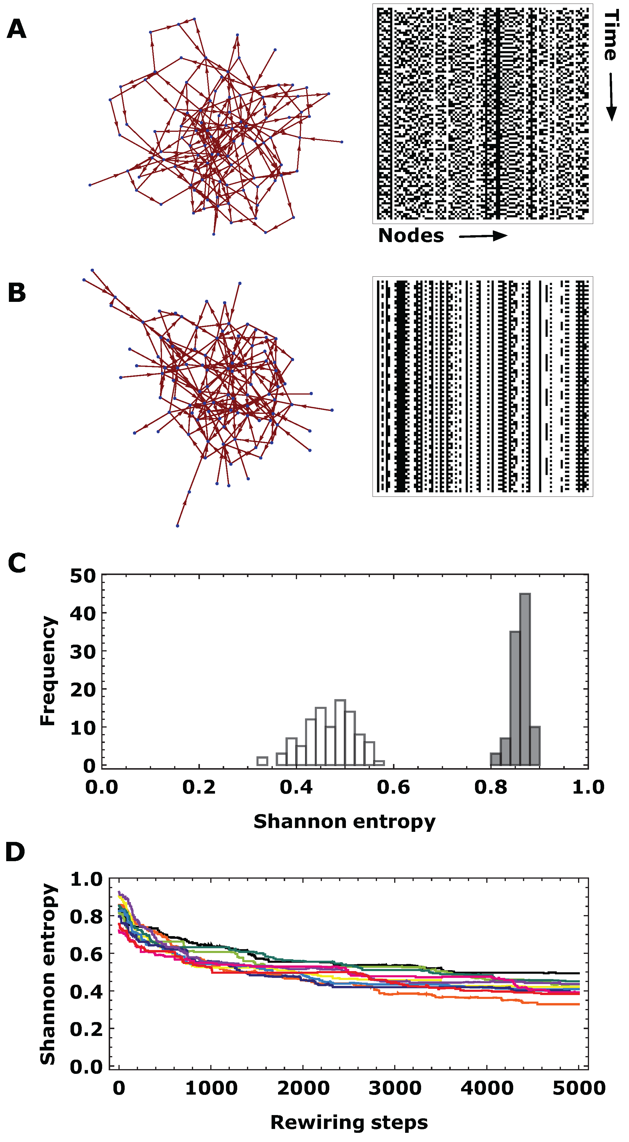
  • Generate a directed ER graph with 100 nodes and about 200 links ( p 0.02).
  • Implement the cellular automaton defined in Equation (1) with κ = 0.3 , 200 timesteps and 100 different initial conditions.
  • Evaluate the (node-)averaged Shannon and word entropies as defined in Equations (2) and (3).
  • Apply a single rewiring step by randomly choosing a directed link and connect either the start or the end of the link to a randomly chosen node. Ensure that the new link does not yet exist and that the resulting graph is weakly connected (i.e., the undirected version of the graph is connected). Repeat steps 2–3 for the new graph.
  • Accept the new graph (labeled i) and discard graph i 1 , if the entropy differences Δ E S ( i ) = E S ( i 1 ) E S ( i ) 0 . If Δ E S ( i ) < 0 , accept the new graph with probability P i = e x p ( Δ E S ( i ) / T ( i ) ) . Here, we choose a linear cooling scheme T ( i ) = T ( 0 ) ( 1 i / s ) where s denotes the number of evolution steps (5000) and T ( 0 ) denotes the initial temperature, which we choose as 0.01. If graph i is accepted, continue with step 2, otherwise choose a new graph i with step 4.
Summarizing, we employ simulated evolution to modify graph topology in such a way that some desired dynamical features (here: low entropies) are enhanced. Such a simulated evolution should not be confused with biological evolution in any sense. Even though both may be interpreted as a search in high-dimensional space, simulated evolution depends on a specific objective function rather than “biological fitness”. Also, diverse physical, chemical and biological constraints enter biological evolution biasing the “search” in a multitude of ways.
It is not clear whether the final result (i.e., the set of evolved networks) is rather shaped directly by the objective function or rather by the details of the search method. In other words, we cannot be certain to discover the same properties of successful networks, if (hypothetically) all possible successful networks were enumerated, rather than searching them via a simulated-evolution strategy.

3. Results

3.1. Evolved Networks

We explore a simulated evolution of graphs towards binary dynamics with low average entropy. The entropy of the time series observed at a node in the graph here serves as a measure for the local complexity of the dynamics, as well as a way of assessing, whether local perturbations are predominantly amplified or dampened at this site in the graph [35].
We follow the protocol outlined in Section 2.5 and generate in each run 10 ER graphs with N = 100 nodes, a directed link probability of p = 2 N 1 0.02 and thus, about 200 links. Each of the graphs is probed with 100 initial conditions. The CA from Equation (1), when implemented on this graph, gives rise to complex spatiotemporal patterns. One graph and one 2D projection of the pattern from the ensemble of graphs and patterns is shown in Figure 4A. After 5000 evolution steps, both the graph topology and the patterns have changed considerably (see Figure 4B). The mean Shannon entropy of the initial graphs are peaked well above 0.8 (see Figure 4C, filled bars), while the reduced complexity of the time series results in a distribution of entropies around 0.5 (Figure 4, white bars). The decreasing Shannon entropy for 10 different initial graphs is shown in Figure 4D.

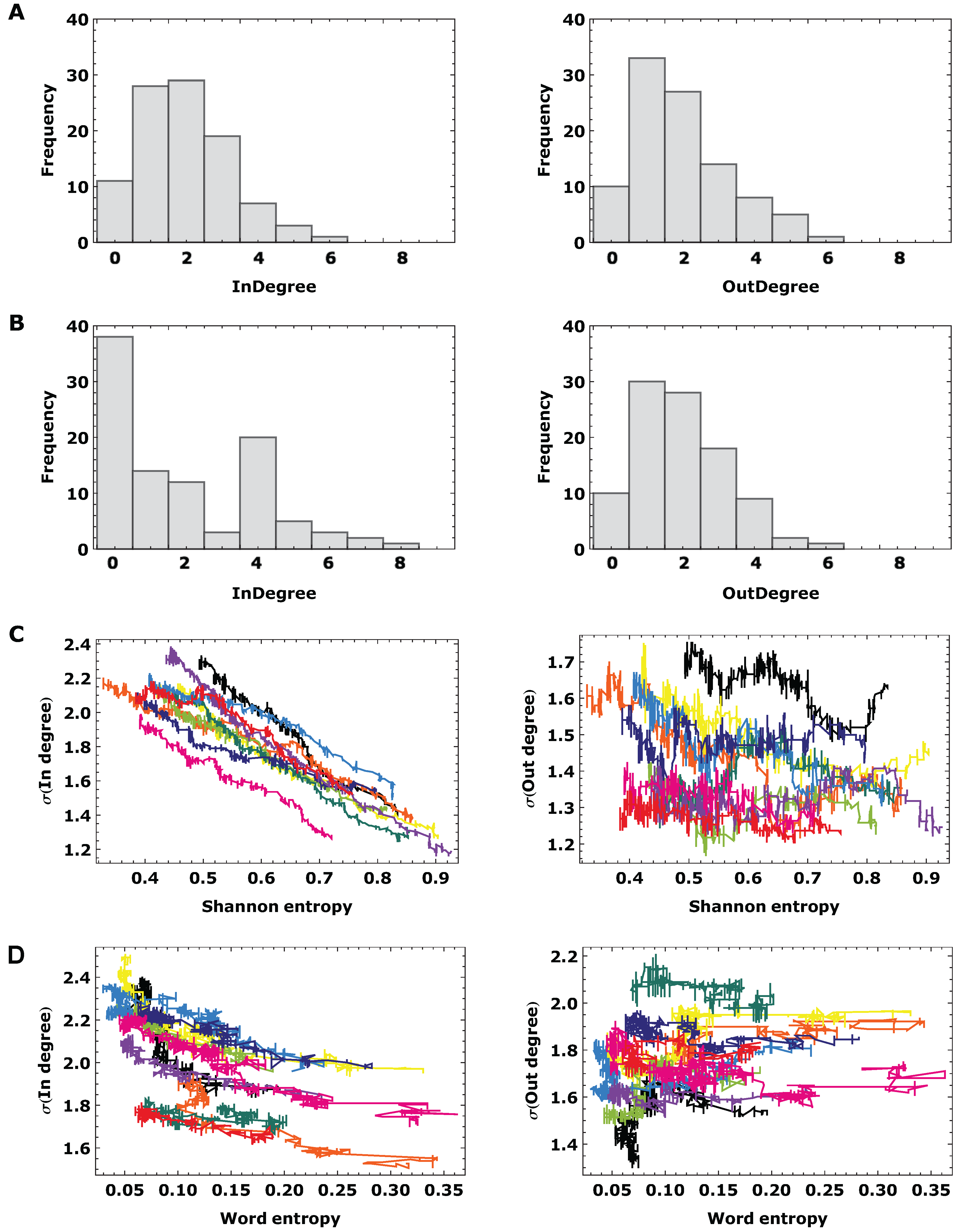
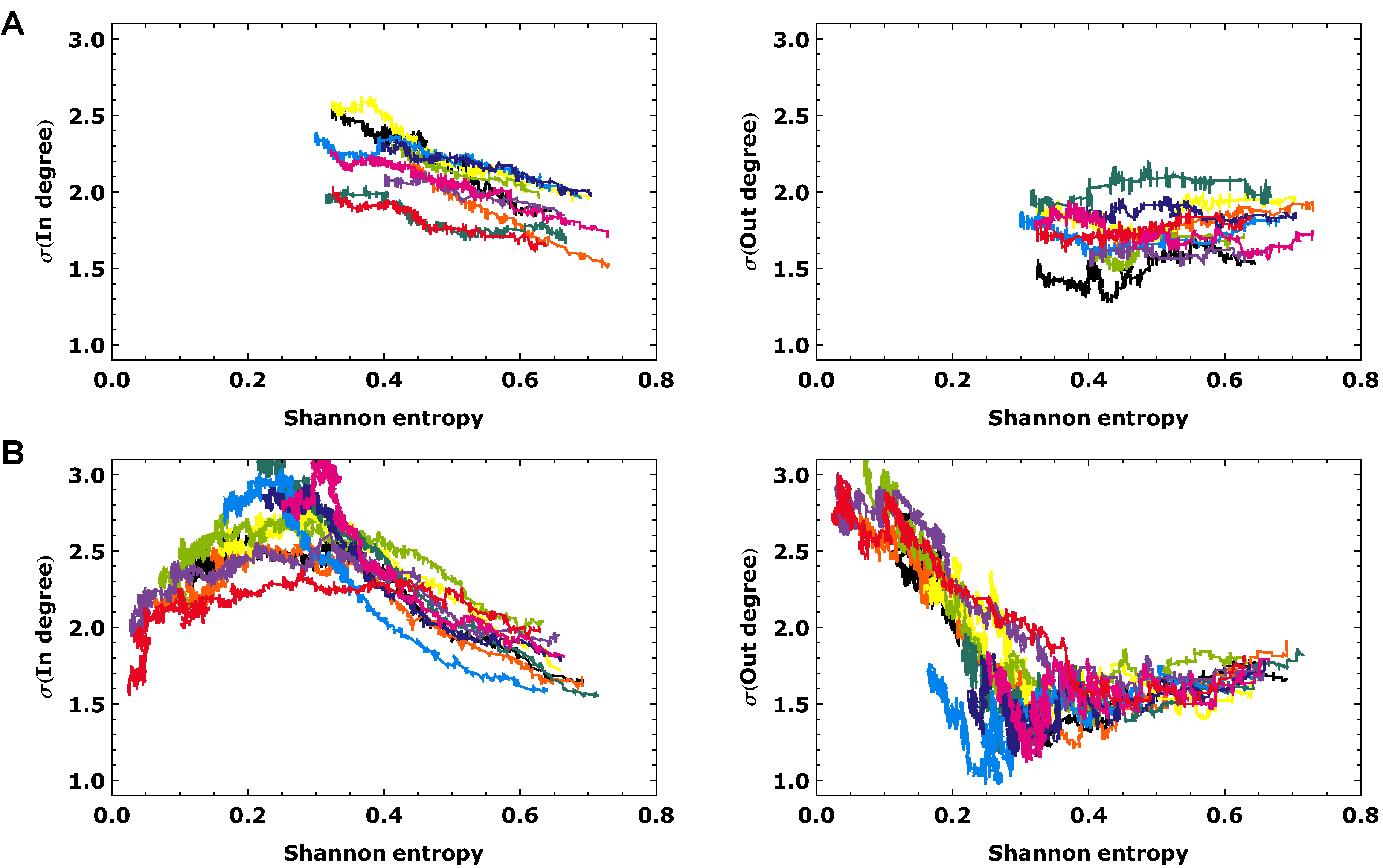
3.2. Topological Analysis

What is the topological imprint (i.e., the systematically altered topological properties) of the changed dynamic potential of the evolved graphs? We compare the in-degree and out-degree distributions of initial and evolved graphs and find remarkable differences. The out-degree distribution of the evolved graph (Figure 5B, right) follows a binomial distribution with a peak at two, just like for the distributions of the initial graph (Figure 5A). The in-degree distribution of the evolved graph however has a peak shifted to 1 and longer tail towards higher degrees. The emergence of nodes with low degree at the periphery of the graph and hubs in the center is already discernable in the graph plot in Figure 4B. To correlate the changes in the in-degree distribution with the dynamic potential of the graph, as measured by the Shannon entropy, we show ten trajectories with 5000 evolution steps in Figure 5C. Interestingly, the standard deviation of the in-degree distribution increases in a linear fashion with decreasing Shannon entropy. At the same time no clear effect on the out-degree is observable (Figure 5C right). Finally, we study the changes of the word entropy and its correlation with the graph degrees in Figure 5D: While the word entropy decreases along with the selection on low Shannon entropies, the correlation between dynamic readout and topological measure is less clear in this case.
Figure 4. Simulated evolution. (A) We implement the dynamic probe (1) on a directed Erdős-Rényi (ER) graph with 100 nodes and 200 links (left), resulting in a spatio-temporal pattern (right). We quantify the dynamic potential of the graph with the average Shannon entropy from Equation (2) of 100 runs with random initial conditions. We evolve the network by a single rewiring step, where either the start point or the end point of a randomly chosen link is attached to a new, randomly chosen node. If the Shannon entropy (again we take the mean over 100 runs with random initial conditions) of the new network is smaller, we accept it. If it is higher, we accept it with a certain temperature-dependent probability (see Section 2.6 for details) to avoid local minima. (B) An evolved network and spatiotemporal pattern after 5000 evolution steps. (C) Shannon entropies for the ER graph (black) and the evolved network (white). (D) Decreasing Shannon entropy for 10 initial ER graphs. Colors denote different runs.
Entropy 14 00993 g004
Figure 5. Topological changes. (A) In-degree and out-degree distribution for an initial ER graph and (B) an evolved networks. The in-degree distribution significantly broadens (p-value < 0.008, Kolmogorov–Smirnov test) during the evolution. (C) The standard deviation of the in-degree distribution increases linearly with decreasing Shannon entropy (we show the same 10 runs as in Figure 4), while the out-degree distribution shows no clear change. (D) The word entropy decreases accordingly, with a less clear correlation between degree and E W signature. Colors denote different runs.
Entropy 14 00993 g005
It should be noted that the details of the simulated-evolution procedure affect properties of the evolved networks. In particular, the distribution of initial conditions and the exact model for the starting networks have a considerable impact. Figure 6 provides some intuition on the amount of variability we can expect. Different schemes of averaging over initial conditions during the simulated evolution have been studied: Scheme 1 (standard setup): entropies are averaged over 100 random initial conditions; at each generation, new initial conditions are selected. This is evaluated in Figure 4, Figure 5, and Figure 6A. Scheme 2: entropies are averaged over 100 random initial conditions; these initial conditions remain the same across the whole simulated evolution. This is the configuration behind Figure 6B.
Figure 6. 10 simulated evolution runs with 10000 steps, selecting for low Shannon entropy E S with different schemes of averaging over initial conditions during the evolution. (A) In each generation, a new set of 100 initial conditions is selected. This leads to a linear increase of the standard deviation of the k in with decreasing Shannon entropy. (B) In contrast, if we keep the set of 100 initial conditions during the whole evolution, a maximum of σ ( k in ) is reached at E S 0.3 . Further evolution of the networks leas to a sharpening of the in-degree distribution and, at the same time, a broadening of the out-degree distribution.
Entropy 14 00993 g006
In both cases, the broadening of the in-degree distribution (increase of the standard deviations σ ( k in ) with decreasing Shannon entropy E S ) is clearly seen in Figure 6A,B (left). However, in the case of 100 constant initial conditions (Scheme 2), the in-degree distribution is maximally broad at E S 0.3 (Figure 6B). If we evolve the networks further, the in-degree distribution again becomes slightly narrower, while at the same time, the out-degree distribution broadens, in contrast to Scheme 1, where the out-degrees seem to be unaffected by the simulated evolution. These trajectories suggest a two-step process: First, the in-degree distribution is broadened to optimize the networks towards low entropy. In a second step, the out-degree distribution broadens as the networks adapt to the specific set of 100 initial conditions. It would be interesting to see how the trajectories of the two schemes converge for all 2 N initial conditions—that is, the limit where Scheme 1 and 2 become identical.
In contrast to the results described so far, selection on the word entropy E W does not lead to a broadening of the degree distribution (data not shown; see, e.g., Figure 5D for an indication of the much lesser impact of E W on the spread of the degree).
Ever since the formulation of scale-free graphs [55], broad degree distributions have been associated with robustness against random node failure. Here we find that, additionally, the broadening of the degree distribution is associated with a more regular (low-entropy) dynamics as well.
In addition to the degree distribution, we looked at a large number of other topological properties of the evolved networks. In particular, the low-entropy networks do not deviate systematically from their unevolved counterparts in their modularity or their degree correlations. They also do not display a non-random triad significance profile (see [5]) indicative of small network motifs [6].
It should be noted that, as with many simulated-evolution studies, our investigation contains several technical parameters that can in principle have a strong impact on the topological features of the evolved networks. We checked that the broadening of the degree distribution is not affected by variations of initial networks, mutation depth (i.e., the number of rewiring steps before evaluating the entropies again) and temperature.

4. Conclusions

Cellular automata on graphs are a parameter-efficient framework for exploring the relationship between network architecture and dynamics from the perspective of pattern formation. Theories of spatiotemporal pattern formation have contributed fundamentally to a deep understanding of natural processes, particularly in biology. One striking example is Turing’s concept of reaction-diffusion processes [56], which has a vast range of applications—from biology to social systems. At the same time, these theories (or classes of models) are well embedded in the broader framework of self-organization. Very much in the light of [57] and [34] our principal goal is to understand what the network equivalents of classical spatiotemporal patterns are, and how, e.g., the presence of loops and feedbacks in networks relate the processes behind spatiotemporal patterns to the theory of complex systems.
Here we have shown some relations between network architecture and dynamics (reviewed from previous work and obtained with the simulated-evolution scheme presented in Section 3), which is interesting in its own right as cornerstones on the road towards a theory of dynamical processes on graphs. At the same time, this set of relations facilitates an evolutionary interpretation of real biological networks in the light of dynamical function.
An analysis of topologically sensitive rules (see [16]) with analytical tools as developed in [58,59] or the basin entropy [60] may reveal state space changes associated with topological modifications. Such analyses can elucidate dynamic properties also relevant for regulatory dynamics of biological networks, which have been successfully modeled with CA approaches (see, e.g., [61,62]). From this perspective, our framework provides a means to comprehensively study the sensitivity of a system to topological perturbations and associated rule space modifications.
How can the entropies derived from our dynamic-probe studies be interpreted from a functional perspective? In the cellular automaton from [35], the density of 1s in the neighborhood determines whether the state of a node flips. It is clear that these dynamics do not correspond directly to any specific biological process. However, it is possible to arrive at a biological interpretation of the dynamics in two different ways:
  • Indirectly, these binary dynamics measure whether fluctuations in the neighborhood of a node will propagate to the node under consideration, or whether they will rather be dampened out. In fact, when one discusses a simple system of linear ODEs on the graph and monitors transient lengths, one sees a clear correlation with our two entropies.
  • When formally re-writing the CA update rules as coupled ODEs (with, e.g., a switching of a state corresponding to a large term in the corresponding ODE) one could in some cases allow for a biological interpretation of the update rules, as the right-hand sides of such ODE systems can be viewed as a “list” of biological processes to the dynamics of the system at hand.
We believe that the application of dynamic probes is a particularly helpful tool for studying dynamical constraints imposed by network topology.
It is clear that many facets of this topic cannot be solved within the framework of this work, i.e., the control of technical parameters in the simulated evolution, the full characterization of the evolved networks, and a (more) complete understanding of low-entropy signatures. We take some of these facets as an inspiration for continuing this line of work. Quite clearly we hope that eventually the evolved, low-entropy networks can be characterized more clearly, also giving mechanistic insight into the way topological properties of a graph regulate the complexity of the dynamics.
Broad degree distributions, like the ones encountered in scale-free graphs [55] and many real biological and technical networks, are often associated either with specific graph construction processes (like preferential attachment) or with robustness against random failures [2]. Even though the degree distributions of the evolved graphs obtained here are far from comparable with the power-law distributions of scale-free graphs (also due to the small size of the graphs investigated here), it is striking that in our study the broadening of the degree distribution is related to the functional requirement of low entropies.

Acknowledgements

This work was supported by the Helmholtz Alliance on Systems Biology (project ‘CoReNe’). MH gratefully acknowledges support from Deutsche Forschungsgemeinschaft (grant HU-937/6) and from Volkswagen Foundation (program ‘Complex networks as a phenomenon across disciplines’).

References

  1. Jeong, H.; Tombor, B.; Albert, R.; Oltvai, Z.N.; Barabási, A.L. The large-scale organization of metabolic networks. Nature 2000, 407, 651–654. [Google Scholar]
  2. Barabási, A.L.; Oltvai, Z.N. Network biology: Understanding the cell’s functional organization. Nat. Rev. Genet. 2004, 5, 101–113. [Google Scholar] [CrossRef] [PubMed]
  3. Ravasz, E.; Somera, A.L.; Mongru, D.A.; Oltvai, Z.N.; Barabási, A.L. Hierarchical organization of modularity in metabolic networks. Science 2002, 297, 1551–1555. [Google Scholar] [CrossRef] [PubMed]
  4. Guimera, R.; Amaral, L. Functional cartography of complex metabolic networks. Nature 2005, 433, 895–900. [Google Scholar] [CrossRef] [PubMed]
  5. Milo, R.; Itzkovitz, S.; Kashtan, N.; Levitt, R.; Shen-Orr, S.; Ayzenshtat, I.; Sheffer, M.; Alon, U. Superfamilies of evolved and designed networks. Science 2004, 303, 1538–1542. [Google Scholar] [CrossRef] [PubMed]
  6. Alon, U. Network motifs: Theory and experimental approaches. Nat. Rev. Genet. 2007, 8, 450–461. [Google Scholar] [CrossRef] [PubMed]
  7. Lesne, A. Complex networks: From graph theory to biology. Lett. Math. Phys. 2006, 78, 235–262. [Google Scholar] [CrossRef]
  8. Strogatz, S. Exploring complex networks. Nature 2001, 410, 268–276. [Google Scholar] [CrossRef] [PubMed]
  9. Rosvall, M.; Bergstrom, C. Maps of random walks on complex networks reveal community structure. Proc. Natl. Acad. Sci. USA 2008, 105, 1118–1123. [Google Scholar] [CrossRef] [PubMed]
  10. Arenas, A.; Díaz-Guilera, A.; Pérez-Vicente, C.J. Synchronization reveals topological scales in complex networks. Phys. Rev. Lett. 2006, 96, 114102. [Google Scholar] [CrossRef] [PubMed]
  11. Newman, M.E. Modularity and community structure in networks. Proc. Natl. Acad. Sci. USA 2006, 103, 8577–8582. [Google Scholar] [CrossRef] [PubMed]
  12. Alexander, R.P.; Kim, P.M.; Emonet, T.; Gerstein, M.B. Understanding modularity in molecular networks requires dynamics. Sci. Signal. 2009, 2, pe44. [Google Scholar] [CrossRef] [PubMed]
  13. Wagner, A. Circuit topology and the evolution of robustness in two-gene circadian oscillators. Proc. Natl. Acad. Sci. USA 2005, 102, 11775. [Google Scholar] [CrossRef] [PubMed]
  14. Schulman, L.; Gaveau, B. Dynamical distance: Coarse grains, pattern recognition, and network analysis. Bull. Sci. Math. 2005, 129, 631–642. [Google Scholar]
  15. Marr, C.; Hütt, M. Topology regulates pattern formation capacity of binary cellular automata on graphs. Physica A 2005, 354, 641–662. [Google Scholar] [CrossRef]
  16. Marr, C.; Hütt, M.T. Outer-totalistic cellular automata on graphs. Phys. Lett. A 2009, 373, 546–549. [Google Scholar] [CrossRef]
  17. Kashtan, N.; Alon, U. Spontaneous evolution of modularity and network motifs. Proc. Natl. Acad. Sci. USA 2005, 102, 13773–13778. [Google Scholar] [CrossRef] [PubMed]
  18. Kashtan, N.; Noor, E.; Alon, U. Varying environments can speed up evolution. Proc. Natl. Acad. Sci. USA 2007, 104, 13711. [Google Scholar] [CrossRef] [PubMed]
  19. Kashtan, N.; Parter, M.; Dekel, E.; Mayo, A.E.; Alon, U. Extinctions in heterogeneous environments and the evolution of modularity. Evolution 2009, 63, 1964–1975. [Google Scholar] [CrossRef] [PubMed]
  20. Kaluza, P.; Mikhailov, A.S. Evolutionary design of functional networks robust against noise. Europhys. Lett. 2007, 79, 48001. [Google Scholar] [CrossRef]
  21. Kaluza, P.; Ipsen, M.; Vingron, M.; Mikhailov, A. Design and statistical properties of robust functional networks: A model study of biological signal transduction. Phys. Rev. E 2007, 75, 15101. [Google Scholar] [CrossRef]
  22. Kaluza, P.; Vingron, M.; Mikhailov, A. Self-correcting networks: Function, robustness, and motif distributions in biological signal processing. Chaos 2008, 18, 026113. [Google Scholar] [CrossRef] [PubMed]
  23. Kobayashi, Y.; Shibata, T.; Kuramoto, Y.; Mikhailov, A.S. Evolutionary design of oscillatory genetic networks. Eur. Phys. J. B 2010, 76, 167–178. [Google Scholar] [CrossRef]
  24. von Neumann, J. The general and logical theory of automata. In Design of Computers, Theory of Automata and Numerical Analysis; J. von Neumann, Collected Works; Taub, A.H., Ed.; Pergamon Press: London, UK, 1963; Volume 5, pp. 288–326. [Google Scholar]
  25. Gardner, M. Mathematical games: The fantastic combinations of John Conway’s new solitaire game “Life”. Sci. Am. 1970, 10, 120. [Google Scholar] [CrossRef]
  26. Dresden, M.; Wong, D. Life games and statistical models. Proc. Natl. Acad. Sci. USA 1975, 72, 956–960. [Google Scholar] [CrossRef] [PubMed]
  27. Wolfram, S. Statistical mechanics of cellular automata. Rev. Mod. Phys. 1983, 55, 601. [Google Scholar] [CrossRef]
  28. Wolfram, S. Universality and complexity in cellular automata. Physica D 1984, 10, 1. [Google Scholar] [CrossRef]
  29. Deutsch, A.; Dormann, S. Cellular Automaton Modeling and Biological Pattern Formation; Birkhäuser: Boston, MA, USA, 2005. [Google Scholar]
  30. Schulman, L.; Seiden, P. Percolation and galaxies. Science 1986, 233, 425–431. [Google Scholar] [CrossRef] [PubMed]
  31. Seiden, P.; Celado, F. A model for simulating cognate recognition and response in the immune system. J. Theor. Biol. 1992, 158, 329–357. [Google Scholar] [CrossRef]
  32. Marr, C.; Hütt, M. Similar impact of topological and dynamic noise on complex patterns. Phys. Lett. A 2006, 349, 302–305. [Google Scholar] [CrossRef]
  33. Müller-Linow, M.; Marr, C.; Hütt, M.T. Topology regulates the distribution pattern of excitations in excitable dynamics on graphs. Phys. Rev. E 2006, 74, 1–7. [Google Scholar] [CrossRef]
  34. Müller-Linow, M.; Hilgetag, C.C.; Hütt, M.T. Organization of excitable dynamics in hierarchical biological networks. PLoS Comput. Biol. 2008, 4, e1000190. [Google Scholar] [CrossRef] [PubMed]
  35. Marr, C.; Müller-Linow, M.; Hütt, M.T. Regularizing capacity of metabolic networks. Phys. Rev. E 2007, 75, 1–6. [Google Scholar] [CrossRef]
  36. Amaral, L.; Goldberger, A. Emergence of complex dynamics in a simple model of signaling networks. Proc. Natl. Acad. Sci. USA 2004, 101, 15551–15555. [Google Scholar] [CrossRef] [PubMed]
  37. Moreira, A.A.; Mathur, A.; Diermeier, D.; Amaral, L.A.N. Efficient system-wide coordination in noisy environments. Proc. Natl. Acad. Sci. USA 2004, 101, 12085. [Google Scholar] [CrossRef] [PubMed]
  38. Watts, D.J.; Strogatz, S.H. Collective dynamics of ‘small-world’ networks. Nature 1998, 393, 440. [Google Scholar] [CrossRef] [PubMed]
  39. Graham, I.; Matthai, C.C. Investigation of the forest-fire model on a small-world network. Phys. Rev. E 2003, 68, 036109. [Google Scholar] [CrossRef]
  40. Shen-Orr, S.; Milo, R.; Mangan, S.; Alon, U. Network motifs in the transcriptional regulation network of Escherichia coli. Nat. Genet. 2002, 31, 64–68. [Google Scholar] [CrossRef] [PubMed]
  41. Riehl, W.J.; Krapivsky, P.L.; Redner, S.; Segrè, D. Signatures of arithmetic simplicity in metabolic network architecture. PLoS Comput. Biol. 2010, 6, e1000725. [Google Scholar] [CrossRef] [PubMed]
  42. Maslov, S.; Krishna, S.; Pang, T.; Sneppen, K. Toolbox model of evolution of prokaryotic metabolic networks and their regulation. Proc. Natl. Acad. Sci. USA 2009, 106, 9743. [Google Scholar] [PubMed]
  43. Samal, A.; Singh, S.; Giri, V.; Krishna, S.; Raghuram, N.; Jain, S. Low degree metabolites explain essential reactions and enhance modularity in biological networks. BMC Bioinformatics 2006, 7, 118–118. [Google Scholar] [CrossRef] [PubMed]
  44. Almaas, E. Optimal flux patterns in cellular metabolic networks. Chaos 2007, 17, 026107. [Google Scholar] [CrossRef] [PubMed]
  45. Almaas, E.; Kovács, B.; Vicsek, T.; Oltvai, Z.N.; Barabási, A.L. Global organization of metabolic fluxes in the bacterium Escherichia coli. Nature 2004, 427, 839–843. [Google Scholar] [PubMed]
  46. Basler, G.; Grimbs, S.; Ebenhöh, O.; Selbig, J.; Nikoloski, Z. Evolutionary significance of metabolic network properties. J. R. Soc. Interface 2011. [Google Scholar] [CrossRef] [PubMed]
  47. Basler, G.; Ebenhöh, O.; Selbig, J.; Nikoloski, Z. Mass-balanced randomization of metabolic networks. Bioinformatics 2011, 27, 1397–1403. [Google Scholar] [CrossRef] [PubMed]
  48. Price, N.D.; Reed, J.L.; Palsson, B.O. Genome-scale models of microbial cells: Evaluating the consequences of constraints. Nat. Rev. Microbiol. 2004, 2, 886–897. [Google Scholar] [CrossRef] [PubMed]
  49. Kauffman, K.J.; Prakash, P.; Edwards, J.S. Advances in flux balance analysis. Curr. Opin. Biotechnol. 2003, 14, 491–496. [Google Scholar] [CrossRef] [PubMed]
  50. Feist, A.M.; Palsson, B.O. The growing scope of applications of genome-scale metabolic reconstructions using Escherichia coli. Nat. Biotechnol. 2008, 26, 659–667. [Google Scholar] [CrossRef] [PubMed]
  51. Ma, H.; Zeng, A.P. Reconstruction of metabolic networks from genome data and analysis of their global structure for various organisms. Bioinformatics 2003, 19, 270–277. [Google Scholar] [CrossRef] [PubMed]
  52. Erdős, P.; Rényi, A. On random graphs. Publ. Math. 1959, 6, 290. [Google Scholar]
  53. Trusina, A.; Maslov, S.; Minnhagen, P.; Sneppen, K. Hierarchy measures in complex networks. Phys. Rev. Lett. 2004, 92, 178702. [Google Scholar] [CrossRef] [PubMed]
  54. Kirkpatrick, S.; Gelatt, C.D., Jr.; Vecchi, M.P. Optimization by simulated annealing. Science 1983, 220, 671–680. [Google Scholar] [CrossRef] [PubMed]
  55. Barabasi, A.; Albert, R. Emergence of scaling in random networks. Science 1999, 286, 509. [Google Scholar] [PubMed]
  56. Turing, A. The chemical basis of morphogenesis. Phil. Trans. Roy. Soc. Lond. B Biol. Sci. 1952, 237, 37–72. [Google Scholar] [CrossRef]
  57. Nakao, H.; Mikhailov, A.S. Turing patterns in network-organized activator-inhibitor systems. Nature 2010, 6, 544–550. [Google Scholar] [CrossRef]
  58. Drossel, B. Random Boolean networks. In Reviews of Nonlinear Dynamics and Complexity; Schuster, H.G., Ed.; Wiley: Weinheim, Germany, 2008. [Google Scholar]
  59. Peixoto, T.; Drossel, B. Boolean networks with reliable dynamics. Phys. Rev. E 2009, 80, 056102. [Google Scholar] [CrossRef]
  60. Krawitz, P.; Shmulevich, I. Basin entropy in Boolean network ensembles. Phys. Rev. Lett. 2007, 98, 158701. [Google Scholar] [CrossRef] [PubMed]
  61. Davidich, M.; Bornholdt, S. Boolean network model predicts cell cycle sequence of fission yeast. PLoS One 2008, 3, e1672. [Google Scholar] [CrossRef] [PubMed]
  62. Braunewell, S.; Bornholdt, S. Superstability of the yeast cell-cycle dynamics: Ensuring causality in the presence of biochemical stochasticity. J. Theor. Biol. 2007, 245, 638–643. [Google Scholar] [CrossRef] [PubMed]

