Statistical Information Based Single Neuron Adaptive Control for Non-Gaussian Stochastic Systems

Abstract

Based on information theory, the single neuron adaptive control problem for stochastic systems with non-Gaussian noises is investigated in this paper. Here, the statistic information of the output within a receding window rather than the output value is used for the tracking problem. Firstly, the single neuron controller structure, which has the ability of self-learning and self-adaptation, is established. Then, an improved performance criterion is given to train the weights of the single neuron. Furthermore, the mean-square convergent condition of the proposed control algorithm is formulated. Finally, comparative simulation results are presented to show that the proposed algorithm is superior to the PID controller. The contributions of this work are twofold: (1) the optimal control algorithm is formulated in the data-driven framework, which needn’t the precise system model that is usually difficult to obtain; (2) the control problem of non-Gaussian systems can be effectively dealt with by the simple single neuron controller under improved minimum entropy criterion.

1. Introduction

As a simple and effective controller, the proportional-integral-derivative controller (PID controller), which has advantages in terms of strong robustness, high reliability, good dynamic response and so on, has been widely used in most industrial control systems. Although it attracts many engineers’ attention, even today, the parameters of the traditional PID controller cannot be adjusted adaptively. Satisfactory control quality often cannot be obtained due to the inevitable nonlinearity and disturbances in real processes. Motivated by the structure and function of the cerebral neural networks, artificial neural networks (ANN) were originally developed by McCulloch and Pitts in 1943. For its specific stability of nonlinear adaptive information processing, ANN has been researched extensively by many scholars and engineers to deal with modern complex nonlinear systems [1,2,3]. It is well known that most multi-layer neural networks adopt S-type functions, which increase the amount of calculation. In order to meet the requirements of fast neural control processes, the single neuron adaptive control strategy was proposed in [4]. Besides the ability of self-learning and self-adaptation, the single neuron adaptive control strategy has real time ability due to its rapid numerical calculation. The model-free adaptive control system formed by single neuron, because of its simple structure, has been studied and some results of learning algorithm and applications can be found (see e.g., [5,6]).

Stochastic systems can be regarded as reasonable ones due to the inevitable randomness in practical industrial processes. Under the assumption that the noises obey a Gaussian distribution, some mature control strategies have been established, such as minimum variance control and linear quadratic Gaussian (LQG) control. However, the disturbances in practical systems are not necessarily non-Gaussian; moreover, nonlinearity in stochastic control systems could lead to non-Gaussian randomness even if the disturbances obey a Gaussian distribution. For this case, the stochastic distribution control (SDC) method was proposed by Wang [7], where the shape of the output probability density function (PDF) rather than the output itself was considered. Recently, a linear-matrix-inequalities (LMI)-based convex optimization algorithm was used for the control of output PDF, filtering and fault detection for non-Gaussian systems by Guo and Wang in [8], where a B-spline was utilized to approximate the output PDF. As such, the PDF was characterized by the weights and selected B-splines. Accordingly the evolution of the PDF can be represented by the state equation of the weights [9,10,11]. However, not all the PDFs of the outputs are measurable. Several new methods were introduced to overcome these problems by investigating the closed-loop performance characterized by the entropy of the output tracking error [12,13,14,15]. Since the exact models are difficult to obtain in practical industrial processes, it is a promising approach to use the only statistic information of systems input and output data. [16,17,18] presented the estimation of the α-order Renyi’s entropy directly from the on-line output data. In [19], by using the above data-driven method, a novel run-to-run control methodology was proposed for semiconductor processes with uncertain metrology delay.

Motivated by the above results, in this paper a single neuron adaptive controller, which is a model-free controller, is developed for stochastic systems with non-Gaussian disturbances. The proposed control strategy is based on an improved minimum entropy criterion of closed loop stochastic systems. Our contributions are twofold. First, we present a simple control algorithm with the absence of the exact system model. Second, an improved non-Gaussian performance index is formulated to train the weights of the single neuron. Based on the optimal weights, the control algorithm could drive the tracking error approximating to zero with small deviation.

The remainder of the paper is organized as follows: the structure of the single neuron controller is illustrated in Section 2. An improved performance index including the information potential of the closed loop tracking error, the mean value of squared tracking error and constraints on control input energy is introduced. Using the non-parametric estimation of the PDF of tracking errors, the performance index is then obtained in Section 3. By minimizing the proposed performance index using the decreasing gradient method, weights of the single neuron are updated in Section 4. In addition, mean-square convergent condition of the proposed control algorithm is formulated. Comparative simulation results are given to illustrate the efficiency and validity of the proposed method in Section 5.

2. Structure of Single Neuron Adaptive Controller

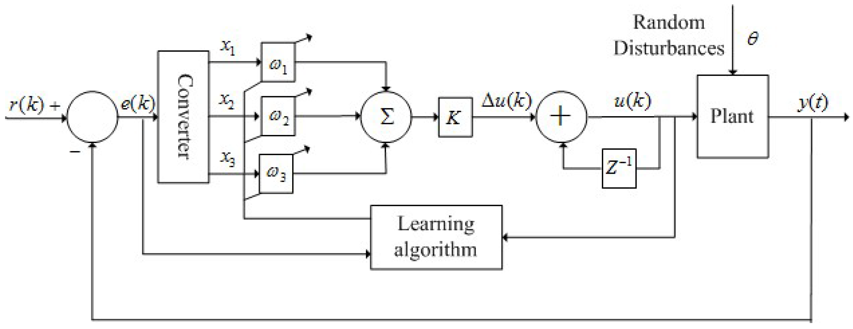
The general scheme of the single neuron adaptive control system is illustrated as Figure 1.

Figure 1. The schematic diagram of a single neuron adaptive control system.

Figure 1. The schematic diagram of a single neuron adaptive control system.

In Figure 1, $\theta$ is the non-Gaussian random disturbance involved in the system. $r(k)$ and $y(k)$ are set-point and controlled variable respectively, $e(k)=r(k)-y(k)$ is the tracking error in the closed loop control system. The control input $u(k)$ can be expressed as:

$$u(k)=u(k-1)+K{\displaystyle \sum _{l=1}^3{\omega }_l(k)x_l(k)}/\Vert \mathrm{\Sigma }\Vert$$

(1)

where $\mathrm{\Sigma }={\displaystyle \sum _{l=1}^3{\omega }_l}$, $K>0$ is proportional coefficient of neuron. ${\omega }_l(k)$ $(l=1,2,3)$ stands for the weight corresponding to each input. $x_l(k)(l=1,2,3)$ is the input of the neuron coming from the tracking error $e(k)$ and can be defined as follows:

$$\{\begin{array}{l}{x}_1=e(k)\\ x_2=e(k)-e(k-1)\\ x_3=e(k)-2e(k-1)+e(k-2)\end{array}$$

(2)

Due to the non-Gaussian disturbances $\theta$ involved in the systems, it is necessary to utilize an appropriate performance index to characterize the randomness of the tracking error. Accordingly the main task is to train the weights by minimizing the given performance function so as to drive the tracking error approximation to zero with small randomness.

3. Improved Minimum Entropy Criterion

Since the disturbances in most control systems are not necessarily Gaussian, the variance of the output tracking error would not be sufficient to characterize the performance of the tracking error dynamic systems. Therefore, an alternative measure of uncertainty, entropy, is given to construct the performance index for measuring the dispersion of the stochastic systems. Ideally, small entropy of the tracking error means the error has narrow and sharp PDF. Owing to the computational efficiency of its non-parametric estimator, Renyi’s quadratic entropy ($H_{\alpha }$, $\alpha =2$) is selected here. It can be expressed by the following definition:

$$H_k=-\log {\displaystyle {\int }_{-\infty }^{+\infty }{\gamma }_{e_k}^2(z)dz=-\log V_k}$$

(3)

where $V_k={\displaystyle {\int }_{-\infty }^{+\infty }{\gamma }_{e_k}^2(z)dz}$ is defined as the information potential [17]. It is clear from Equation (3) that Renyi’s quadratic entropy is a monotonic function of the information potential. Hence, in order to simplify computational complexity, the inverse of quadratic information potential is used instead of Renyi’s entropy.

In order to make the tracking error approach zero, the mean value should be considered. Furthermore, since the tracking error may be positive or negative, thus the mean value of the square error should also be included in the performance index:

$$E(e_k^2)={\displaystyle {\int }_{-\infty }^{+\infty }{z}^2{\gamma }_{e_k}(z)dz}$$

(4)

Since control inputs in practical control systems are always constrained by physical limitations of actuators, the magnitude of the control input should be minimized too. Above all, the whole performance function can be formulated as the weighted sum of inverse of the information potential of tracking error, the square of tracking error and the constrains on control input:

$$J_k=R_1\frac{1}{V_k}+R_{2}E(e_k^2)+\frac{1}{2}{R}_3{u}_k^2$$

(5)

In order to calculate the performance index, it is necessary to estimate the PDF of closed-loop tracking error ${\gamma }_{e_k}$ from error sequences $\{e_1,e_2,\cdots ,e_N\}$ within a receding window whose width is $N$. The PDF of the tracking error can be estimated by Parzen windowing technique:

$${\widehat{\gamma }}_{e_k}(x)=\frac{1}{N}{\displaystyle \sum _{i=1}^N\kappa (x-e_i,{\sigma }^2)}$$

(6)

where $\kappa (x,{\sigma }^2)=\frac{1}{\sqrt{2\pi }\sigma }\exp (-\frac{x^2}{2{\sigma }^2})$ is the Gaussian kernel function, ${\sigma }^2$ and $N$ represent typical symmetric variance and the total data number, respectively. Thus the quadratic Renyi’s entropy can be obtained as follows:

$$H(e(k))=-\log \frac{1}{N^2}{\displaystyle \sum _{i=1}^N({\displaystyle \sum _{j=1}^N\kappa (e_i-e_j,2{\sigma }^2)})}$$

(7)

Subsequently, the quadratic information potential and the mathematical expectation of the tracking error can be formulated from samples within the receding window:

$$V(e(k))=\frac{1}{N^2}{\displaystyle \sum _{i=1}^N({\displaystyle \sum _{j=1}^N\kappa (e_i-e_j,2{\sigma }^2)})}$$

(8)

$$E(e^2(k))=\frac{1}{N}{\displaystyle \sum _{i=1}^N{e}_i^2}$$

(9)

Finally, the performance index can be calculated in the following way:

$$\begin{array}{cc}\hfill J(k)& =R_1\frac{1}{V(e(k))}+R_{2}E(e^2(k))+\frac{1}{2}{R}_3{u}^2(k)\hfill \\ & R_1\frac{1}{\frac{1}{N^2}{\displaystyle \sum _{i=1}^N\left({\displaystyle \sum _{j=1}^N\mathsf{{\rm K}}(e_i-e_j,2{\sigma }^2)}\right)}}+R_2\frac{1}{N}{\displaystyle \sum _{i=1}^N{e}_i^2}+\frac{1}{2}{R}_3{u}^2(k)\hfill \end{array}$$

(10)

4. Optimal Control Algorithm and Stability Analysis

4.1. Computation of Control Input

The purpose of the single neuron adaptive stochastic distribution controller design is to find out a set of optimal weighting coefficient $w_l(k)(l=1,2,3)$ to minimize the performance index Equation (10). As far as this controller concerned in this paper, it is a nonlinear optimization problem that can be solved using the gradient algorithm:

$$\mathsf{\Delta }{\omega }_l(k)={\omega }_l(k+1)-{\omega }_l(k)=-{\eta }_l\frac{\partial J(k)}{\partial {\omega }_l(k)}$$

(11)

$$\begin{array}{cc}\hfill \frac{\partial J(k)}{\partial {\omega }_l}=& -\frac{R_1}{2V^2(e(k))N^2{\sigma }^2}{\displaystyle \sum _{i=1}^N{\displaystyle \sum _{j=1}^N(e_i-e_j)\kappa (e_i-e_j,2{\sigma }^2)\cdot (\frac{\partial e_i}{\partial {\omega }_l}-\frac{\partial e_j}{\partial {\omega }_l})}}\hfill \\ & +2R_2{\displaystyle \sum _{i=1}^N{e}_i\frac{\partial e_i}{\partial {\omega }_l}}+R_{3}u(k)\frac{\partial u_k}{\partial {\omega }_l}\hfill \end{array}$$

(12)

$$\frac{\partial e(k)}{\partial {\omega }_l}=-\frac{\partial y(k)}{\partial {\omega }_l}=-\frac{\partial y(k)}{\partial u(k)}\cdot \frac{\partial u(k)}{\partial {\omega }_l}=-\frac{\partial y(k)}{\partial u(k)}\cdot \frac{\partial \mathsf{\Delta }u(k)}{\partial {\omega }_l}$$

(13)

where ${\eta }_l(l=1,2,3)$ is the learning factor. The Jacobian information $\frac{\partial y(k)}{\partial u(k)}$ can be replaced by sgn$\frac{\partial y(k)}{\partial u(k)}$ or calculated by model prediction algorithm of the plant. The influence made by this approximation method can be compensated by adjusting the learning rate. Since $\Vert \mathrm{\Sigma }\Vert$ changes gently, the derivation can be regarded as a constant. Therefore, we have:

$$\frac{\partial \mathsf{\Delta }u(k)}{\partial {\omega }_l}=\{\begin{array}{cc}e(k),\hfill & \hfill l=1\\ e(k)-e(k-1),\hfill & \hfill l=2\\ e(k)-2e(k-1)+e(k-2),\hfill & \hfill l=3\end{array}$$

(14)

the weights ${\omega }_l(l=1,2,3)$ can be updated by Equations (11–14). Then the optimal control algorithm can be obtained from Equation (1).

Remark Denote $W={\left[\begin{array}{ccc}{\omega }_1& {\omega }_2& {\omega }_3\end{array}\right]}^T$, $\eta =diag\{{\eta }_1,{\eta }_2,{\eta }_3\}$, then the weight can be updated by:

$$W(k+1)=W(k)-\eta \frac{\partial J(k)}{\partial W(k)}=W(k)-\eta \nabla J(k)$$

(15)

2.1. Mean-Square Convergence Analysis

In order to analyze the convergence of improved minimum error entropy control algorithm, we consider a quadratic approximation for the performance index $J(k)$ by employing a Taylor series expansion truncated at the linear term for the gradient around the optimal weight vector:

$$J(k)=J_{W^{\ast }}(k)+\frac{1}{2}{\tilde{W}}^T(k)R\tilde{W}(k)$$

(16)

where the optimal solution is defined as $W^{\ast }=\arg \underset{W}{\min }J(k)$, $\tilde{W}(k)=W^{\ast }-W(k)$ and $R:={\nabla }^{2}J(k)$.

Theorem 1

Assume that $J(k)$ is a quadratic surface with a Taylor series approximation given by Equation (16). To ensure mean-square convergence of the control algorithm, a necessary condition is:

$$0<{\eta }_l<\frac{2}{{\lambda }_l}(l=1,2,3)$$

(17)

where ${\lambda }_l(l=1,2,3)$ is the eigenvalue of $R$.

Proof: 

Let $R=Q\mathrm{\Lambda }{Q}^T$, where $Q$ and $\mathrm{\Lambda }$ denote the orthonormal eigenvector and diagonal eigenvalue matrices, respectively. Subtracting both sides of Equation (16) from $W^{\ast }$ and substituting $\nabla J(k)=-R\tilde{W}(k)$ and $R=Q\mathrm{\Lambda }{Q}^T$, it leads to:

$$\begin{array}{cc}\hfill \tilde{W}(k+1)& =\tilde{W}(k)-\eta R\tilde{W}(k)\hfill \\ & =Q[I-\eta \mathrm{\Lambda }]Q^{\text{T}}\tilde{W}(k)\hfill \end{array}$$

(18)

The weight error along the natural modes ($v(k)=Q^T\tilde{W}(k)$) is thus given by:

$$v(k+1)=[I-\eta \mathrm{\Lambda }]v(k)$$

(19)

The expression for the $l^{th}$ mode then becomes:

$$v_l(k+1)=[1-{\eta }_l{\lambda }_l]v_l(k)$$

(20)

hence:

$$v_l^2(k+1)={[1-{\eta }_l{\lambda }_l]}^2{v}_l^2(k)$$

(21)

and:

$${\Vert v_l(k+1)\Vert }^2={[1-{\eta }_l{\lambda }_l]}^2{\Vert v_l(k)\Vert }^2$$

(22)

In order to study the mean-square behavior of the algorithm, we take expectations of both sides of Equation (22) as follows:

$$E{\left[\Vert v_l(k+1)\Vert \right]}^2={[1-{\eta }_l{\lambda }_l]}^{2}E{\left[\Vert v_l(k)\Vert \right]}^2$$

(23)

It is easy to observe from Equation (23) that:

$$\frac{E\left[{\Vert v_l(k+1)\Vert }^2\right]}{E\left[{\Vert v_l(k)\Vert }^2\right]}<1\iff \left|1-{\eta }_l{\lambda }_l\right|\le 1$$

(24)

Since the eigenvalues of the Hessian matrix $R$ are positive, the following condition of mean-square convergence of the control algorithm can be obtained from Equation (24):

$$0<{\eta }_l<\frac{2}{{\lambda }_l}$$

(25)

5. A numerical Example

In order to illustrate the feasibility and efficiency of the presented optimal control algorithm, let us consider the following nonlinear non-Gaussian stochastic system described by:

$$y_k=\frac{1.8y_{k-1}+0.2u_k+0.7u_{k-1}+\sqrt{{\theta }_k}}{{(1+y_{k-1})}^2}$$

(26)

The PDF of random variable ${\theta }_k(k=1,2,\cdots )$ is defined by:

$${\gamma }_{\theta }(z)=\{\begin{array}{l}{[4^{\alpha +\mu +1}\beta (\alpha +1,\mu +1)]}^{-1}{(z+2)}^{\alpha }\\ {(2-z)}^{\mu },z\in (-2,2)\\ 0,otherwise\end{array}$$

(27)

where α = 1 and $\mu =8$. The set-point of system Equation (26) is set to $r(k)=1$. The sampling period is $T=1$ and learning factor ${\eta }_i=0.001(i=1,2,3)$. The weights in Equation (10) are $R_1=0.98$, $R_2=0.01$ and $R_3=0.01$ respectively.

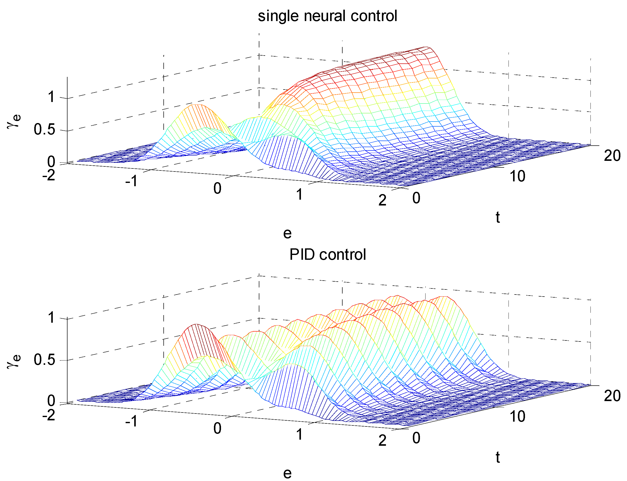
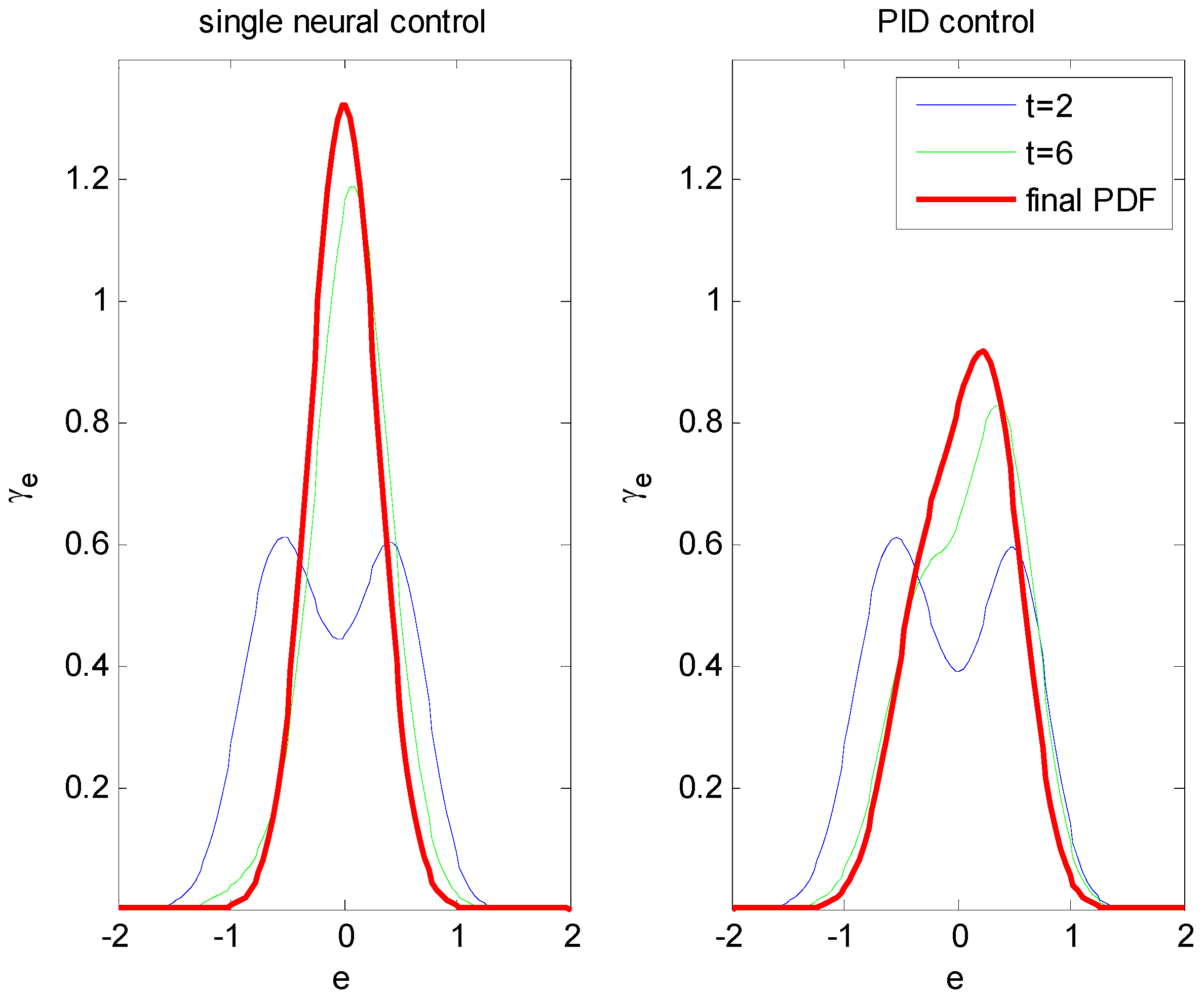
The advantage of the proposed method is shown by comparing with a PID controller whose transfer function is $G_{PID}(s)=k_p+\raisebox{1ex}{$k_i$}\!\left/ \!\raisebox{-1ex}{$s$}\right.+k_{d}s$. The optimal PID parameters are tuned using the Matlab NCD toolbox: $k_p=2.2$, $k_i=0.3$ and $k_d=0.32$. The comparative results are shown in Figure 2, Figure 3, Figure 4, Figure 5 and Figure 6.

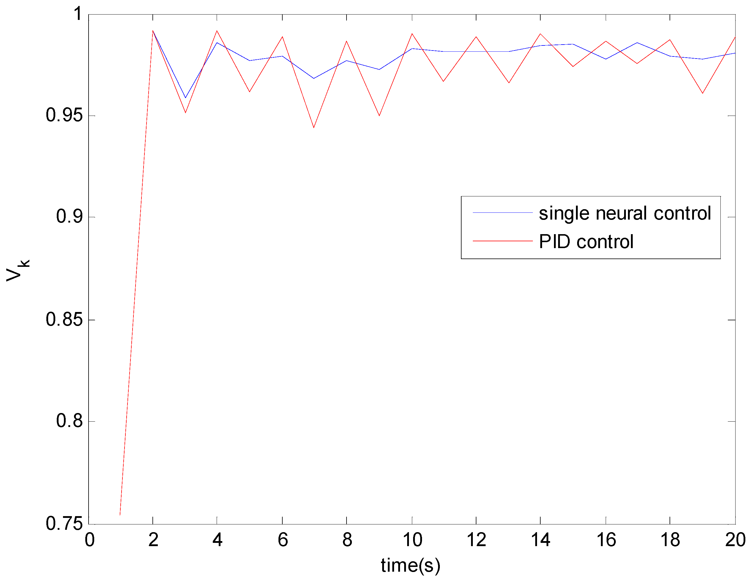
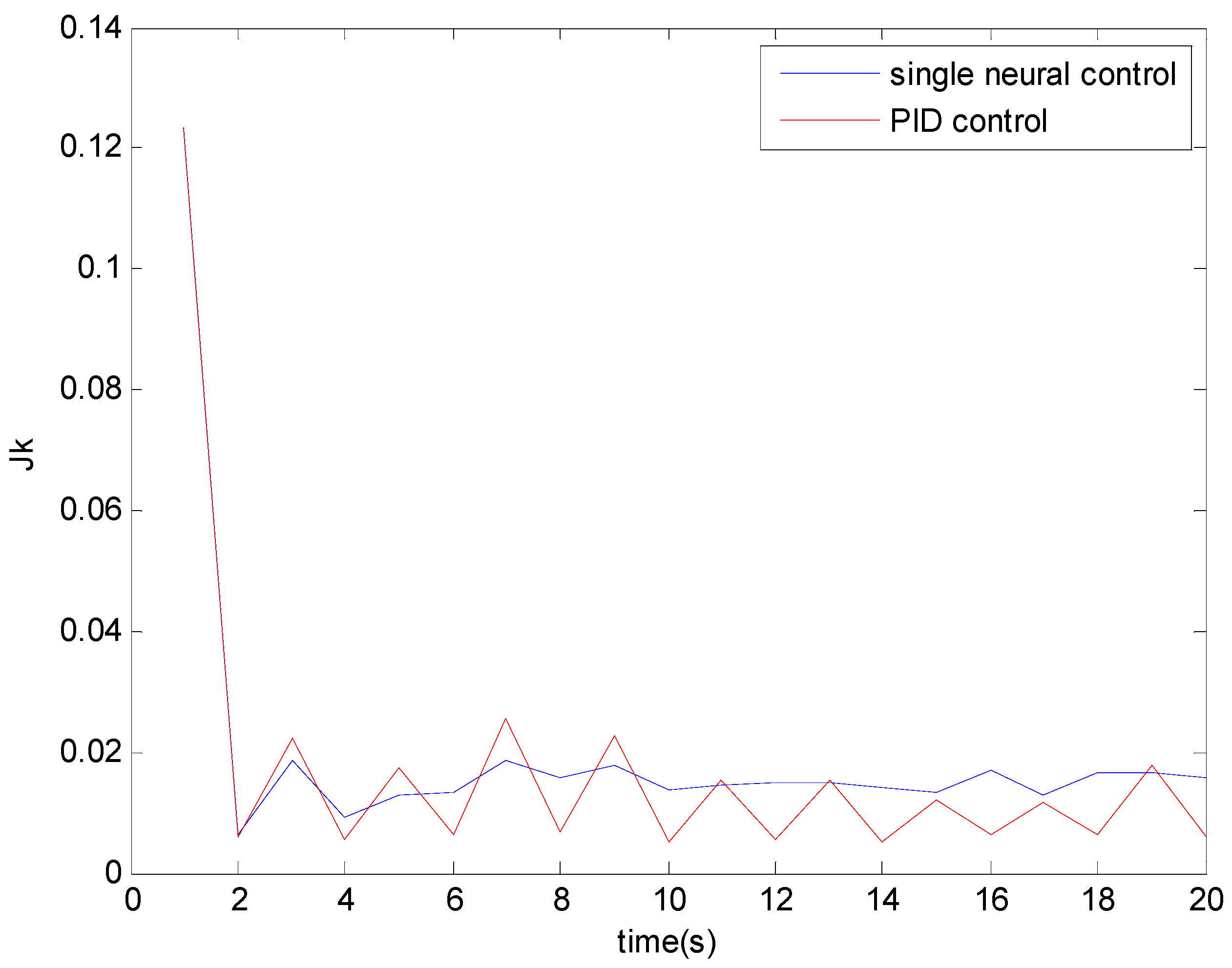
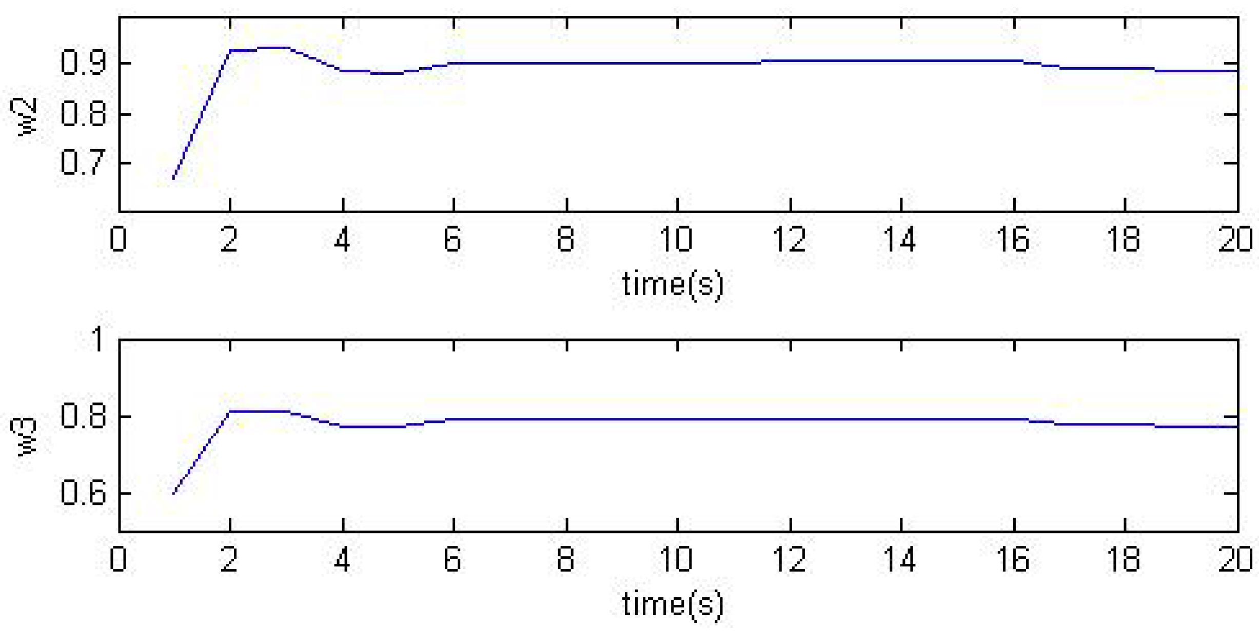
It can be seen from Figure 2 and Figure 3 that the information potentials under PID control and proposed single-neuron adaptive control both increase with time, while the performance indices $J_k$ decrease with time. The variances of the single neuron weights tuned by the proposed performance index are presented in Figure 4. In Figure 5, both the range of tracking errors and PDFs of tracking errors are given. It can be seen that the shapes of PDFs of the tracking errors become narrower along with the increasing of the time. In order to clarify the improvements, the PDFs at several typical instants are shown in Figure 6. It can be shown from Figure 5 and Figure 6 that the proposed single neural adaptive controller can drive the tracking errors toward a smaller randomness. Conversely, the PID control strategy cannot minimize the randomness effectively. From these comparative results, it is obvious that the proposed strategy has better randomness rejection ability than PID control law. Therefore, the proposed control strategy is more suitable for nonlinear stochastic systems with non-Gaussian noises.

Figure 2. Information potentials.

Figure 2. Information potentials.

Figure 3. Performance indices.

Figure 3. Performance indices.

Figure 4. Weights of the single neuron.

Figure 4. Weights of the single neuron.

Figure 5. PDFs of tracking error.

Figure 5. PDFs of tracking error.

Figure 6. PDFs at typical instants.

Figure 6. PDFs at typical instants.

6. Conclusions

This paper has introduced a new statistic information-based single neuron adaptive control algorithm for general control systems with non-Gaussian noises. The performance index of the closed-loop system consists of the information potential of the tracking error, mathematic expectation of squared tracking error and constraints on control input. The optimal control algorithm is obtained by training the neuron weights based on the proposed performance index. Moreover, the implementation of the adaptive single neuron control approach is developed by employing a Parzen windowing technique for estimating PDF of the tracking error. In this work, the given control strategy and the PID control method are both applied to a nonlinear and non-Gaussian stochastic system. Comparative simulation results demonstrate the superiority of the presented control algorithm.