1. Introduction
The concept of entropy has achieved a large consensus as an indicator of complexity of nonlinear signals [
1]. A number of variants of this notion have been proposed in the literature which show different degrees of flexibility, relevance to different problems, efficiency in their computation, as well as theoretical foundations [
2]. The information processing in the brain manifests itself through its global electrical activity, measured by the electroencephalogram (EEG): from an information processing viewpoint this is a multidimensional, non-stationary, nonlinear time series. This assumption is at the basis of the study of EEG through entropy which aims to extract information useful to distinguish among different brain states. In particular, there are variation of EEG related to normal aging and some other aging pathologies that can be detected by means of a complexity analysis. This supports the complexity loss theory for system under stress, for instance, through aging and related diseases [
3,
4]. In this work, the potential of complexity analysis of multidimensional EEG as indicator of AD onset through multi-scale entropic modeling is investigated. This problem has been already faced by several researchers worldwide [
5,
6]. However, the relevance of the complexity of EEG fluctuations with regard to the dynamical changes of the Alzheimer’s Disease (AD) patients has not yet been definitely clarified as possible precursor of the onset of AD, although different studies tend to prefigure this as a practical possibility. This would be extremely important since EEG is a cheap, reproducible way to program a screening and a follow-up of population at risk with clear advantages for the sanitary systems. Thus, further studies are certainly needed and should be encouraged.
Being the EEG a multidimensional signal extracted from a number of correlated channels, it is of high potential interest to be able to exploit its multidimensional nature through techniques that can make inter-channel relations emerge [
7,
8].
The reminder of the paper is organized as follows. In
Section 2, the concept of Permutation Entropy (PE) and the effects of frequency and noise on PE calculation are discussed. In
Section 3, the concept of Multi-Scale analysis is applied to PE; in
Section 4, a multivariate version of PE is introduced. In
Section 5, an original multivariate extension of multi-scale PE is developed.
Section 6 reports some simulation results. Concluding remarks are finally provided in
Section 7.
2. Permutation Entropy (PE)
PE has been introduced as a fast and robust method for extracting information from a time series, with special regard to its complexity [
1]. With this algorithm, the one-dimensional dynamical recording corresponding to the time series is analyzed from a pure ordinal viewpoint [
9]. PE is based on the counting of ordinal patterns (hereafter called “motifs”) that describe the up-and-down in the dynamical signal. The concept of PE is based on the measure of the relative frequencies of the different motifs. Since just ordinal patterns are considered, the amplitude of the signal is actually not relevant, thus yielding a structural robustness to noise. As an interesting by-product, in the study of biological signals (e.g., EEG), this also implies the independence on the choice of the reference electrode [
10]. Accordingly, there is no need of the usual normalization pre-processing step. As an invariant measure, PE is expected to quantify the complexity of the system generating the time series, by discerning the relative change of complexity from limited amount of data. On the other hand, PE reflects just one aspect of the ordinal structure of the signal, thus, some additional investigations are advisable to fully understand both its advantages and limitations [
11].
PE combines the concept of Shannon Entropy to the ordinal pattern analysis through the estimation of the relative frequencies of the ordinal patterns extracted from time series. PE represents an alternative way of measuring similarity among patterns with respect to other types of complexity measurements, like Approximate Entropy and Sample Entropy. In a regular time series, there are lots of similar ordinal patterns; on the contrary, the presence of different patterns occurring with similar relative frequency is indicative of high complexity [
12]. PE is dependent on two-parameters: an embedding dimension,
d, and a time-lag,
τ. Given a scalar time series, y = {y
1, …y
i, …y
N}, an embedding procedure forms data segments where
d is the number of samples belonging to the segment, and
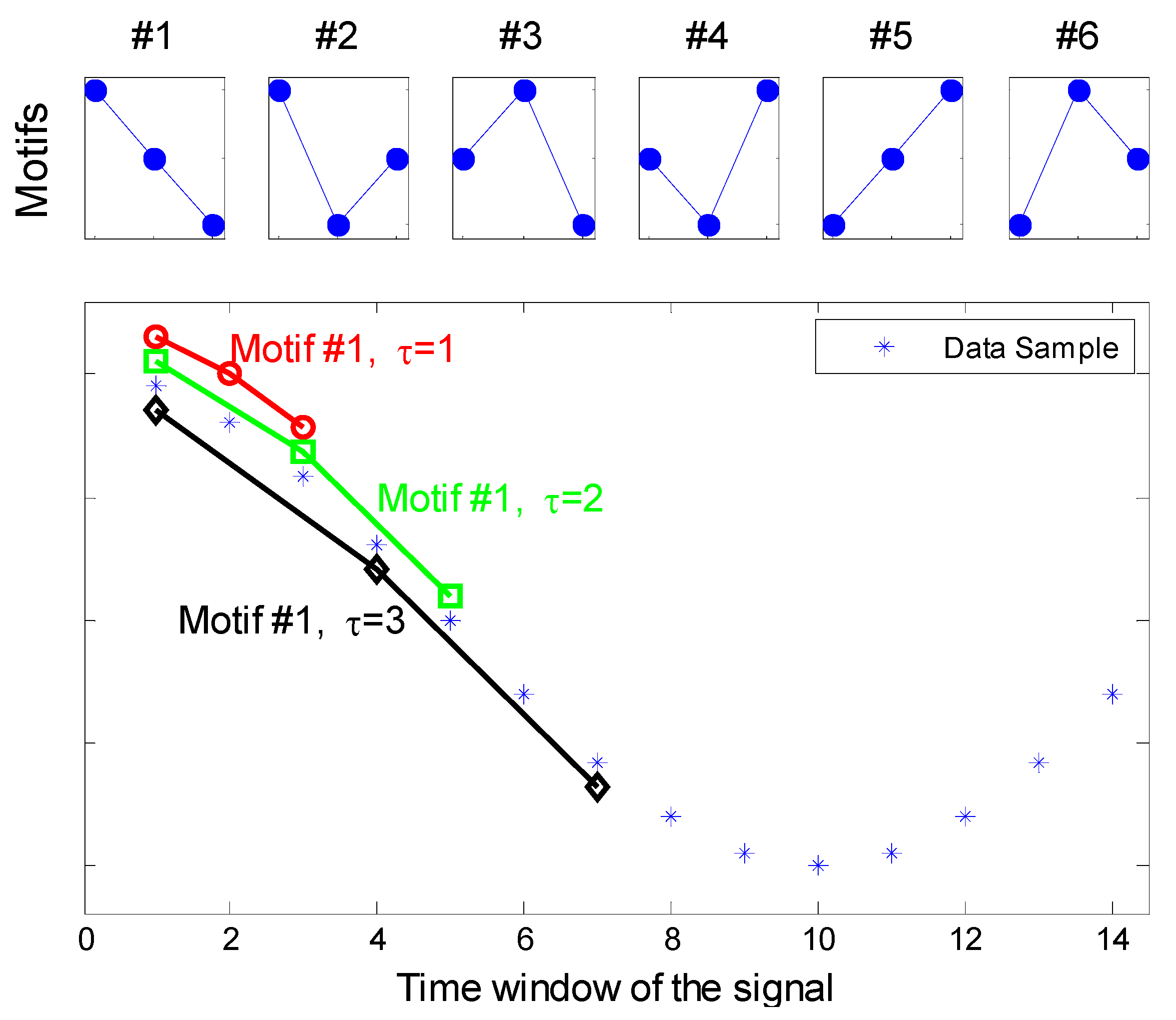
τ represents the distance between the sample points spanned by each section of the motif as depicted in
Figure 1. To compute the PE of the time series, y, first the series of vectors of length d, v
d(n) = [y
n, y
n+1, …, y
(n+d−1)] is derived from the signal samples y
j. Then, v
d(n) is arranged in increasing order of magnitudes: [y
n+j1−1, y
n+j2−1, …, y
n+jn−1]. For
d different samples, there will be
d! possible ordinal patterns, π, which are also called “motifs”. For each single motif π
j, let f(π
j) denote its frequency of occurrence in the time series. The relative frequency is thus:
For fixed embedding dimension d > 2, and fixed time-lag
τ =
, PE is defined as:
where the sum runs over all
d! motifs π. The maximum value of H(d) is log
2(d!), which implies that all motifs have equal probability. The smallest value of H(d) is zero, which implies the time-series is very regular,
i.e., it is a mere repetition of the same basic motif.
Figure 1.
Extraction of ordinal patterns from the signal by varying the time-lag τ (d = 3).
Figure 1.
Extraction of ordinal patterns from the signal by varying the time-lag τ (d = 3).
For convenience, we normalize H(d,
) by its maximum value log
2(d!):
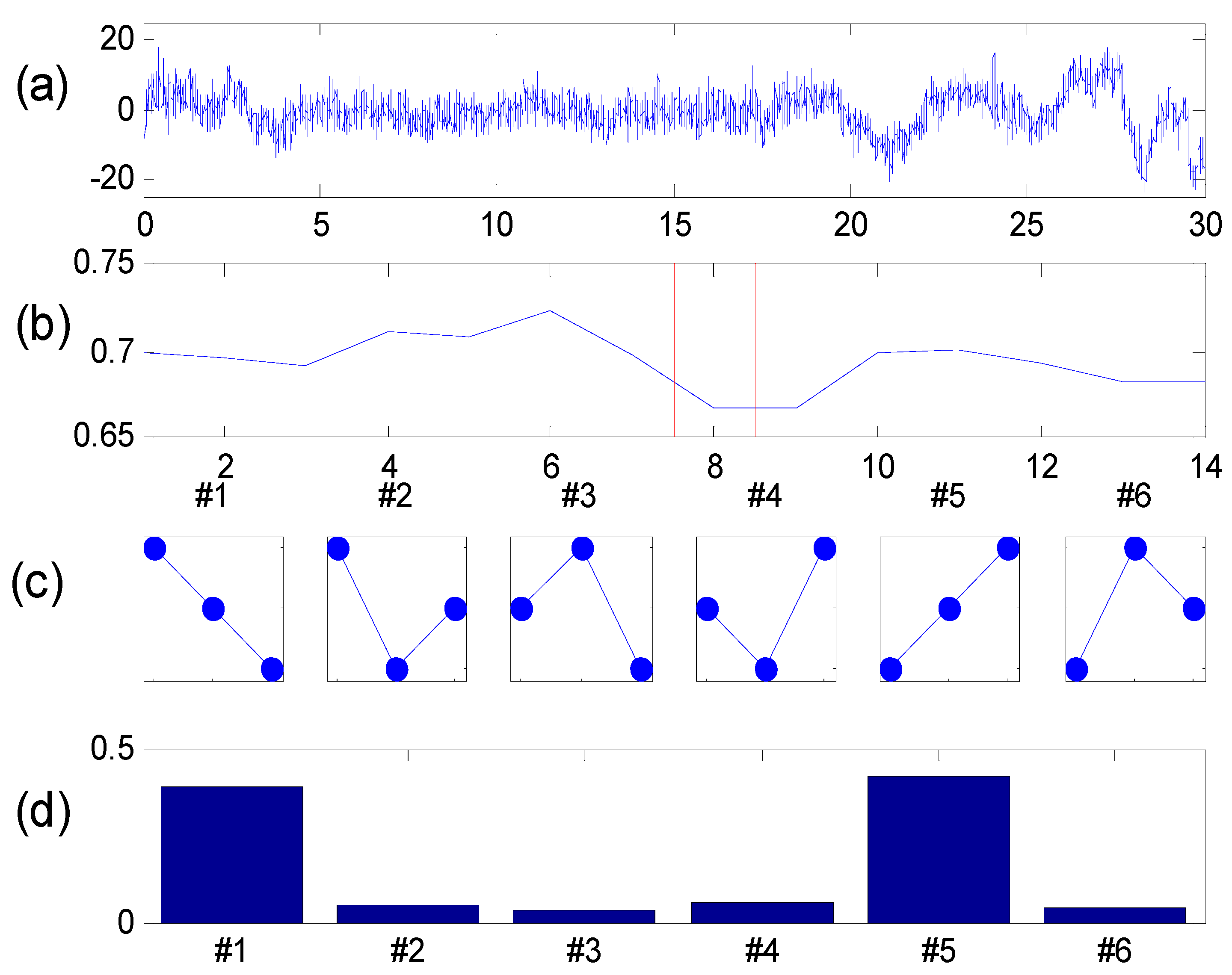
A pictorial description of the PE computation is given in
Figure 2. A 30 s segment extracted from the original EEG time recording for one channel is reported in
Figure 2(a). The time evolution of PE is reported in
Figure 2(b); the six motifs corresponding to d = 3 are depicted in
Figure 2(c) while the relative distribution of p(π) for a selected window is drawn if
Figure 2(d). A similar representation has been proposed in [
13].
Figure 2.
(a) A sample EEG recording extracted from the database; (b) PE time evolution; (c) The six possible motifs for d = 3; (d) Motifs frequency distribution.
Figure 2.
(a) A sample EEG recording extracted from the database; (b) PE time evolution; (c) The six possible motifs for d = 3; (d) Motifs frequency distribution.
2.1. Frequency Dependence of PE
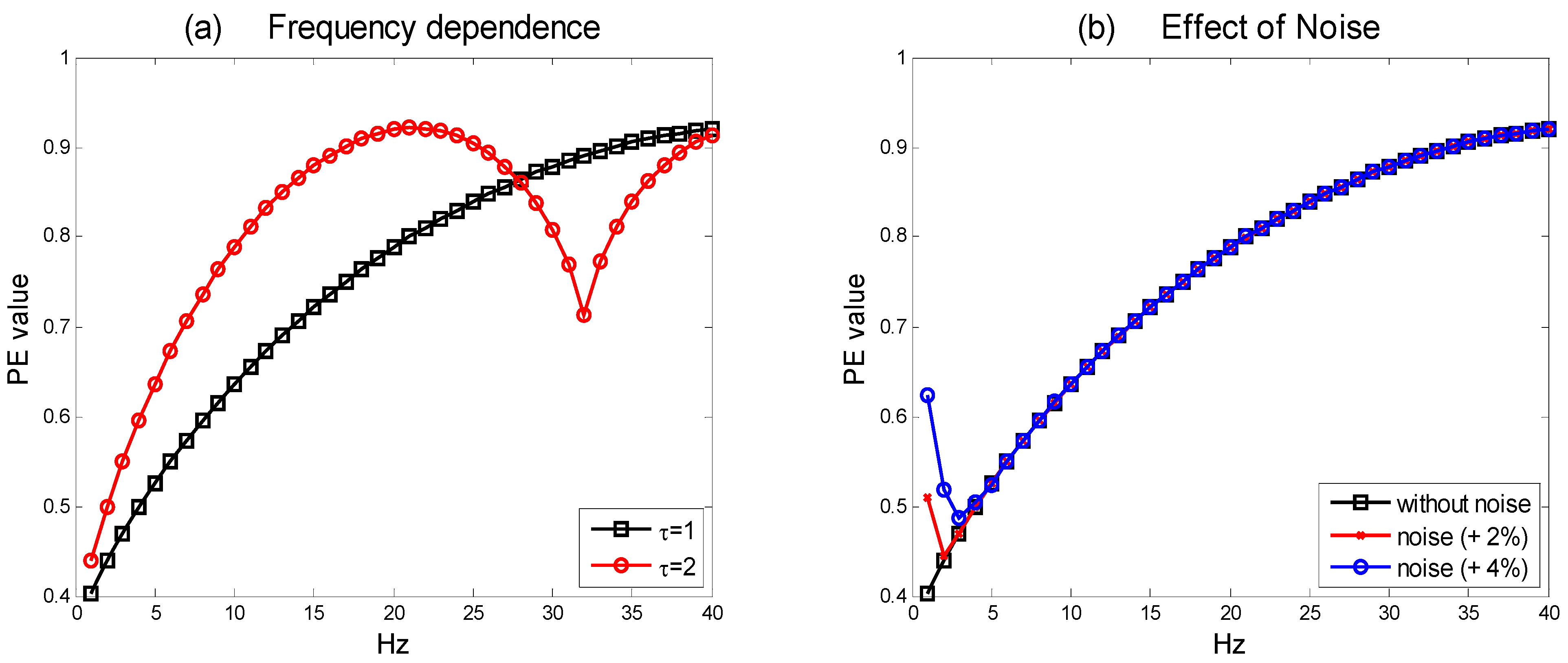
For different choices of the time-lag, τ, PE shows a varying dependence on frequency. To illustrate this effect, we simulate a sequence of pure sine waves time series and then we calculate PE for each of them. The results are reported in
Figure 3(a). As it can be observed, with τ = 1, the PE is monotonically decreasing with decreasing frequency. This yields, in principle, a real advantage for using PE to analyse AD EEG data. In particular, this kind of dependence may reflect the observed “slowing” effect in AD. Early stages of AD (even preclinical) are indeed typically associated with slowing down of resting alpha rhythms, namely, a decrease of the individual alpha frequency peak in power density. This peak is defined as the frequency associated with the strongest EEG power at the alpha range.
Figure 3.
(a) Frequency dependence of PE. The two distributions for τ = 1 and τ = 2 (d = 3, fs = 128 Hz) are reported. The minimum value of PE for τ = 2 is at 32 Hz; (b) The effect of adding white noise on PE calculation (d = 3, τ = 1 and fs = 128 Hz). It is evident the effect on very low frequencies. However, the frequency range of the lowest band considered in EEG signal processing (δ band) is within 2–4 Hz.
PE can explicitly incorporate this kind of behavior. The frequency dependence of PE with τ = 2 is markedly different and more difficult to interpret. In
Figure 3(a), it is also possible to observe that the PE function has a minimum for a frequency that is a fraction of the sampling frequency, f
s. More generally, the time evolution behaviour of the PE for τ = 1, and 2, can be different based on the presence of special signal components. For example, in an EEG signal rich in spindle-like activities, the curves of PE for τ = 1, 2 are very different. Since we are selecting PE as an invariant measure that may capture the “slowing” effect on EEG of AD, in this paper, we limit our simulations to the case of τ = 1. Some authors decided to define a suitably averaged composite PE index that is able to incorporate both the cases, this way exploiting the above described effect [
13].
2.2. Effect of Noise on PE Calculation
The effects of noise on PE have been originally discussed in [
1]. As a consequence of the invariant transformation property of PE, there is a discontinuity near the constant time series. In this case, PE zeroes, since just one motif is represented. If this series is perturbed by noise, the PE value strongly increases. Thus, for some added white noise of sufficient power, the value of PE tends to its maximum at very low frequencies.
Figure 3(b) shows the effect of adding white noise to the simulated sine-wave time series. It is worth noting that, as correctly claimed in [
1], the added noise leaves undisturbed the PE curve after a frequency threshold. This threshold level depends on the power of the noise. The Multi-Scale analysis proposed in this paper can reduce the limitations posed by the described effect, since the coarse-graining procedure has a smoothing effect on the time series. This is relevant in order to leave unaffected the frequency portions of the signals where the “slowing” effect is measured.
3. Multi-Scale Permutation Entropy (MSPE)
The technique of measuring the complexity of a time series through the concept of entropy implies that random sequences attain maximal complexity. In contrast, the complexity analysis can be faced from a “structural” viewpoint: the complexity should not be maximum neither for completely regular nor for completely random sequences. In biological and physiological time series, there are often evident or underlying structural correlations over multiple spatial-temporal levels (scales). Among many other measures, Multi-Scale Entropy (MSE), proposed in 2002 by Costa
et al. [
14] has been shown to be one of the most effective methods that explicitly accounts for such structural effects at multiple time scales present in complex real data. MSE yields a systematic procedure to associate to both fully predictable and uncorrelated random signals a small value of complexity. In contrast, correlated processes show high complexity over different scales. MSE is a method of measuring the complexity of finite length time series that can be appropriately used with different types of entropic measures [
15,
16]. In [
14], the Sample Entropy formulation has been used. Here, we propose to use MSE for evaluating at multiple scales the previously introduced PE. We will limit our analysis from single scale to scale four because of the limited size of the available recordings. As a matter of fact, for PE, a possible way to explore correlations among different scales could be the proper variation of the time lag parameter,
τ. However, it is our opinion that the MSE procedure is easier to interpret with respect to the direct variation of
τ, that implies a fictitious frequency dependence on the sampling frequency. Thus, the usual coarse-graining procedure is implemented, as follows:
- (1)
From the original time series, we derive multiple successive coarse-grained versions by averaging the time data points within non-overlapping time slice of increasing length,
ε, referred to as the scale factor. Each element of the coarse-grained time series, y
j(ε), is calculated as:
The length of each coarse-grained time series is ε times shorter than the original one. For ε = 1, we get the original series;
- (2)
For each scaled series, the PE is calculated. The averaged PE can be plotted as a function of the scale factor, ε.
The selection of different time-lags also implies working on different scales of the time series; we decided to work on a fixed time-lag (τ = 1) in order to avoid unknown cross-effects between the two approaches. In the literature, two papers report on a different way of taking into account time scale variations with reference to PE: a composite index is there derived from two or three different levels. In [
13] the index takes into account two values of the time-lag,
τ, used as a scale factor; in [
11], the authors calculate a multiple scale parameter by considering three successive scales.
4. Multivariate Permutation Entropy (MPE)
The previously discussed MSPE is suitable for single channel time series. Thus, for multiple channel signals, each time series should be considered separately. This kind of procedure may be acceptable just for set of signals that are at least uncorrelated. It is, thus, not the case of scalp EEG, where the volume conduction introduces an integration (correlating) effect at least at a region (lobe) level. Furthermore, the analysis of single channels inevitably implies an information loss related to relevant cross-channel variability.
In this work, a multivariate extension of MSPE is proposed. It implies a suitable definition of PE for multivariate signals, like EEG, and, then, its evaluation over different time scales. A similar concept has been recently introduced by Mandic [
7,
8] for Sample Entropy (MMSE). The method here proposed is quite new and somewhat refers to the original seminal paper of Keller and Laufer [
17]; however, they didn’t take into account variation over multiple scales.
Consider a time window of size T (seconds) of an EEG channel whose sampling frequency is fs = 1/T; each window will thus include (fsT) samples, i.e., data points. For each channel i ∈ [1, m] and for each j ∈ [1, n = d!] (i.e., for each “motif”), count all times s ∈ [1, fsT − d] for which the channel-time pair (i,s) provides the motif j. The relative frequencies pi,j, obtained after dividing the counts by mT, are the entries of a matrix Pt (m,n) =
reflecting the distribution of the motifs in the time slice of length T. It holds
. According to this procedure, the original multivariate time series is transformed into a time dependent matrix from which the relevant statistics and entropies can be easily extracted. In particular, it is easy to compute the marginal relative frequencies describing the distribution of the motifs, as:
for j = 1, …, d!
The cross-channels complexity, representing the Multivariate PE (MPE), can be calculated as the permutation entropy (PE) of p
j:
Through the same matrix, it is also possible to compute the single channel PE, as:
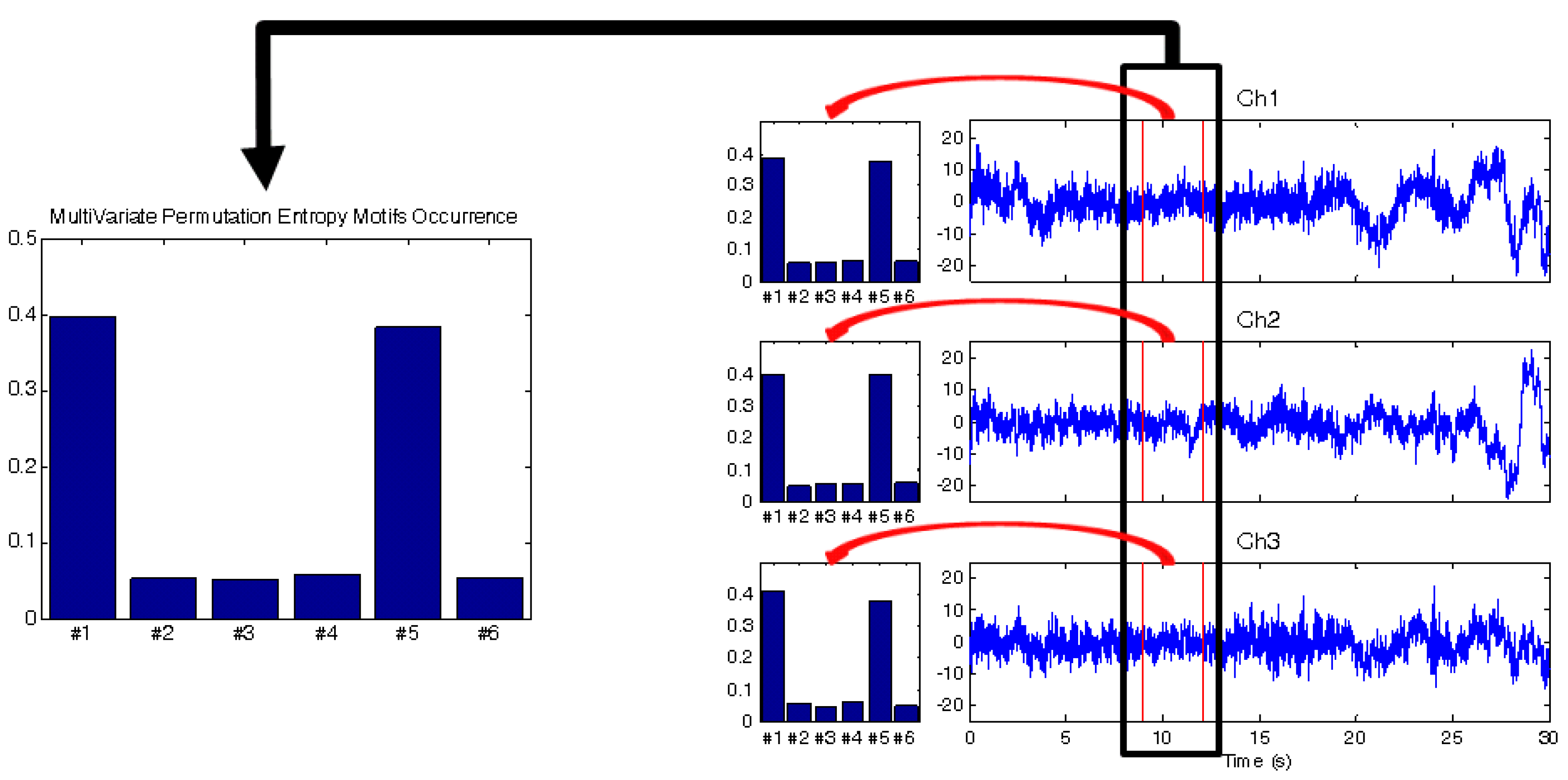
Figure 4 pictorially represents the procedure of MPE computation. A very interesting quantity that can be computed is the Mean Squared Difference between the MPE and the curve obtained by averaging the m single-channel PE. This quantity is called
contingency. It is vanishing if and only if the single channel distributions coincide. If they are highly “similar”, the overall complexity of the time series at time s is the sum of two terms: the mean complexity of the channels and a rest dependent on the inhomogeneity between the channels. A thorough analysis of the impact of contingency on MPE is, however, beyond the scope of the present work.
PE is a measure robust to noise (particularly with respect to high frequency noise): being the MPE substantially a slight variation of an average operation, it can help in absorbing some uncertainties of data acquisition.
MPE can be useful in EEG signal processing since if it is computed on “distant” channels, i.e., on different hemispheres and/or different areas, it may be able to extract cross-channel regularities by highlighting long-range spatial (nonlinear) correlations.
Figure 4.
A pictorial representation of the Multivariate Permutation Entropy (MPE) algorithm. Three different channels and the relative motifs distribution are considered. On the left, the multivariate motifs distribution occurrence.
Figure 4.
A pictorial representation of the Multivariate Permutation Entropy (MPE) algorithm. Three different channels and the relative motifs distribution are considered. On the left, the multivariate motifs distribution occurrence.
6. Complexity Analysis of Different Brain States: Simulation Results
The characterization of brain electrical activities in terms of complexity of the EEG can be a useful tool in different contexts. For example, the time evolution of PE shows evident changing complexity in the transition between inter-ictal and ictal states in the epileptic brain [
10]. In this study, we tested the above discussed algorithms by analyzing the EEG of three different groups of subjects (male and aged between 60–75 years): mild cognitive impaired (MCI) patients, Alzheimer’s Disease (AD) patients and age-matched healthy elderly control (HC). AD is a progressive and irreversible brain disorder of unknown etiology. It is the main cause of dementia in western countries, and it affects 1% of the population aged 60–64 years, but its prevalence increases exponentially with age, so around 30% of people over 85 years suffer from this disease [
15,
20]. Clinically, this disease manifests as a slowly progressive impairment of mental functions whose course lasts several years. Although diagnosing AD definitely can only be done by necropsy, a differential diagnosis with other kinds of dementia, possibly at an early stage, should be attempted. MCI often precedes evident dementing illness: the cognitive impairments of MCI are often not severe enough to exceed standard clinical criteria for AD but in most cases progress toward a clear AD condition. This renders early diagnosis a relevant worldwide emergent question. However, discriminating MCI from HC is generally difficult. The inclusion criteria for enrollment of patients for statistical analysis are mainly standard and at the first lever are based on Mini Mental State Examination (MMSE). The database analyzed in the present study is, however, quite limited: just three cases per category are available. The patients underwent neuro-physical tests that revealed objective evidence of memory impairment. The nine EEG registrations have been collected according to the sites defined by the standard 10–20 international system, at a sampling rate of 200 Hz. The data are band-pass filtered between 0.5 and 32 Hz, so including the relevant bands for AD diagnosis. In the course of the experimental activity, EEG was recorded in rest condition with closed eyes (under vigilance control). The EEG database has been provided by the
IRCCS Centro Neurolesi of Messina, Italy, through a cooperation agreement. A preliminary clinical inspection of the data has been carried out by neurologists of the center for ensuring absence of artifacts and in order to make any relevant clinical observations.
It is quite difficult to carry out any statistical considerations on the basis of the limited available database, for example about the specificity of the diagnosis; however, a statistical validation has been performed in order to quantify the discrimination ability of the different techniques which have been applied to the database of EEG multivariate signals concerning the diagnosis of AD. Some additional information on the problem can be found in [
22]. The PE is previously calculated for each channel. The results are averaged over the three subjects per category. Then, the impact of the scale on the calculation is assessed. More detailed results on the effect of scales on complexity measures are reported elsewhere [
16,
21,
23]. MSPE has been shown to be suitable for single channel time series [
21]. The relevance of a multivariate analysis is here assessed within the multi-scale framework.
The analysis has been carried out by making use of MatLab code which is in part freely available on the Internet. Minor modifications have been implemented for generating the MMSPE curves and for statistical analysis of the data.
Figure 5,
Figure 6 and
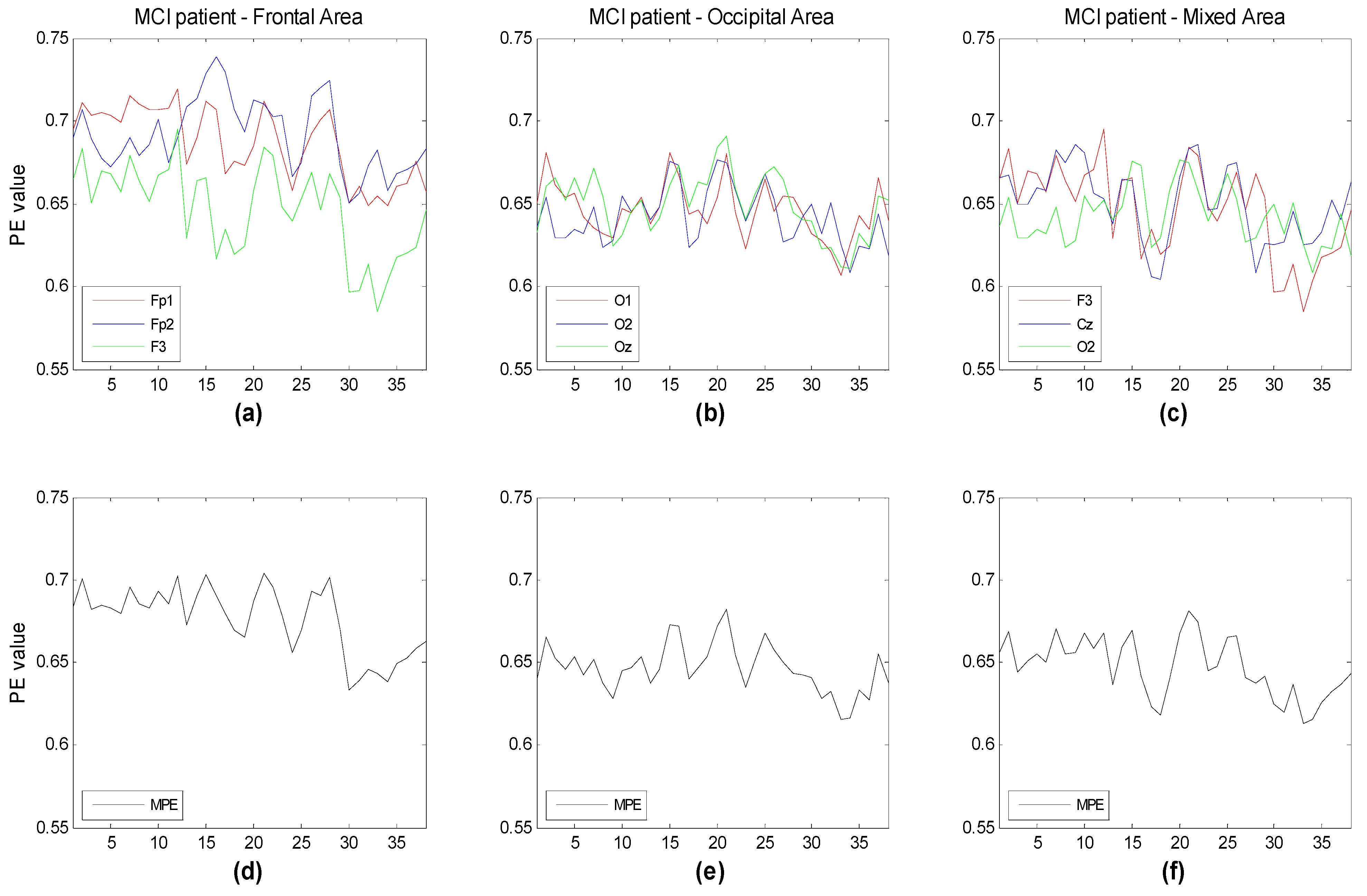
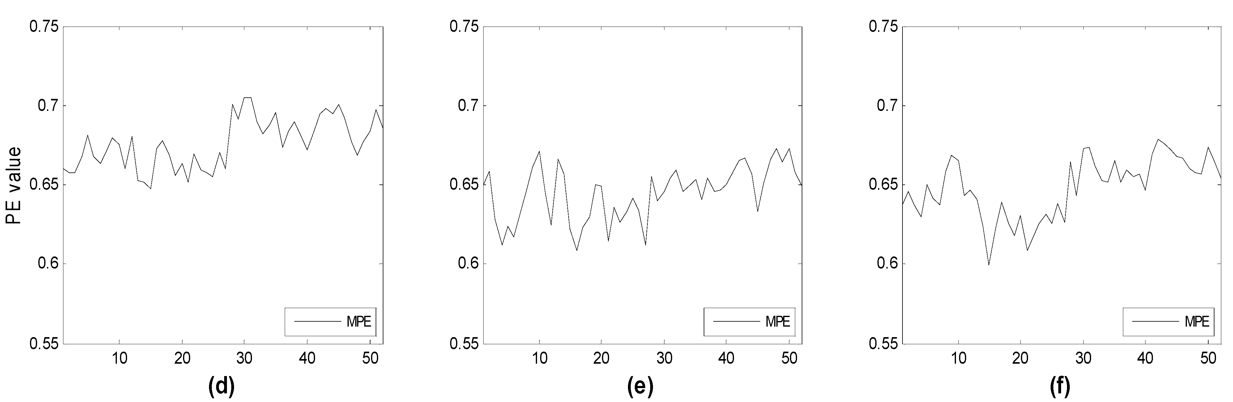
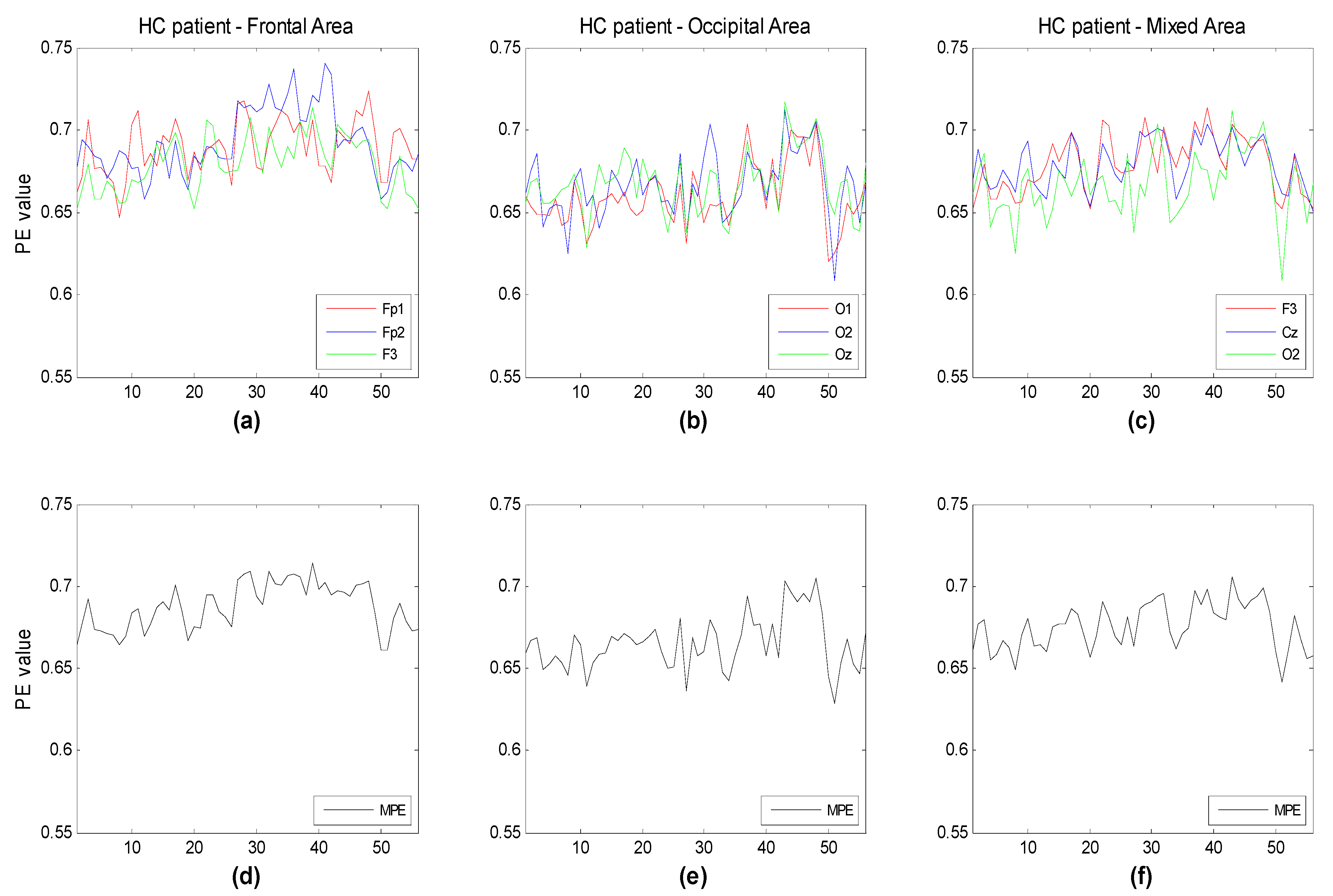
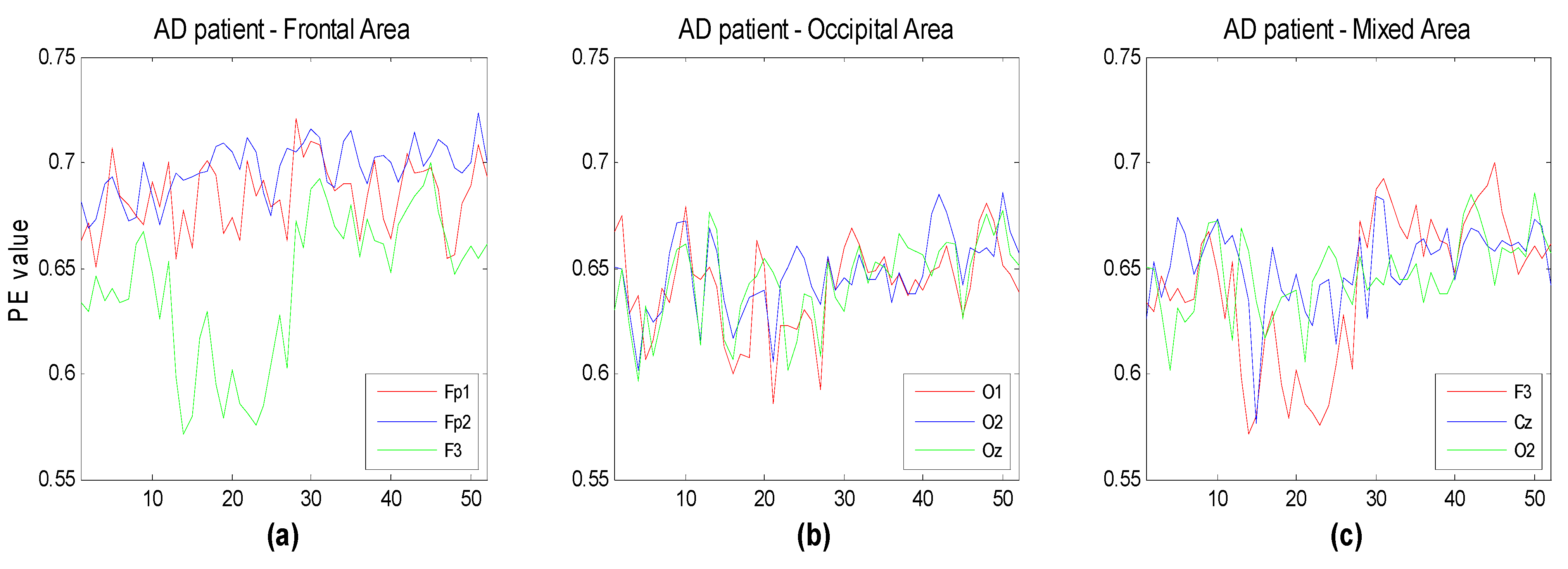
Figure 7 illustrate the time evolution of PE over three channels versus the window number. Each window refers to a segment of the time series of 3 seconds duration. Three different subsets of channels have been considered for the three groups (HC, MCI, AD). The time evolution of the MPE is also reported. One can see that, as expected, the complexity of the signals generally decreases with the severity of the illness, particularly between HC and AD. This is more easily seen looking at the MPE curves. MPE partitions the electrode ensembles in two parts, this way possibly indicating the areas or the subsets of electrodes that may favor a correct diagnosis.
Figure 5.
Time evolution of the computed PE value vs. window number for (a) three frontal electrodes (Fp1, Fp2, F3); (b) three occipital electrodes (O1,O2,Oz); and (c) three electrodes of different area (F3,Cz,O2) compared to the corresponding multivariate PE (MPE); (d–f) for the healthy elderly subjects. Each window spans 3 s of the original time series.
Figure 6.
Time evolution of the computed PE value vs. window number for (a) three frontal electrodes (Fp1, Fp2, F3); (b) three occipital electrodes (O1,O2,Oz); and (c) three electrodes of different area (F3,Cz,O2) compared to the corresponding multivariate PE (MPE); (d–f) for mild cognitive impaired subjects. Each window spans 3 s of the original time series.
Figure 7.
Time evolution of the computed PE value vs. window number for (a) three frontal electrodes (Fp1, Fp2, F3); (b) three occipital electrodes (O1,O2,Oz); and (c) three electrodes of different area (F3,Cz,O2) compared to the corresponding multivariate PE (MPE); (d–f) for subject with Alzheimer’s disease. Each window spans 3 s of the original time series.
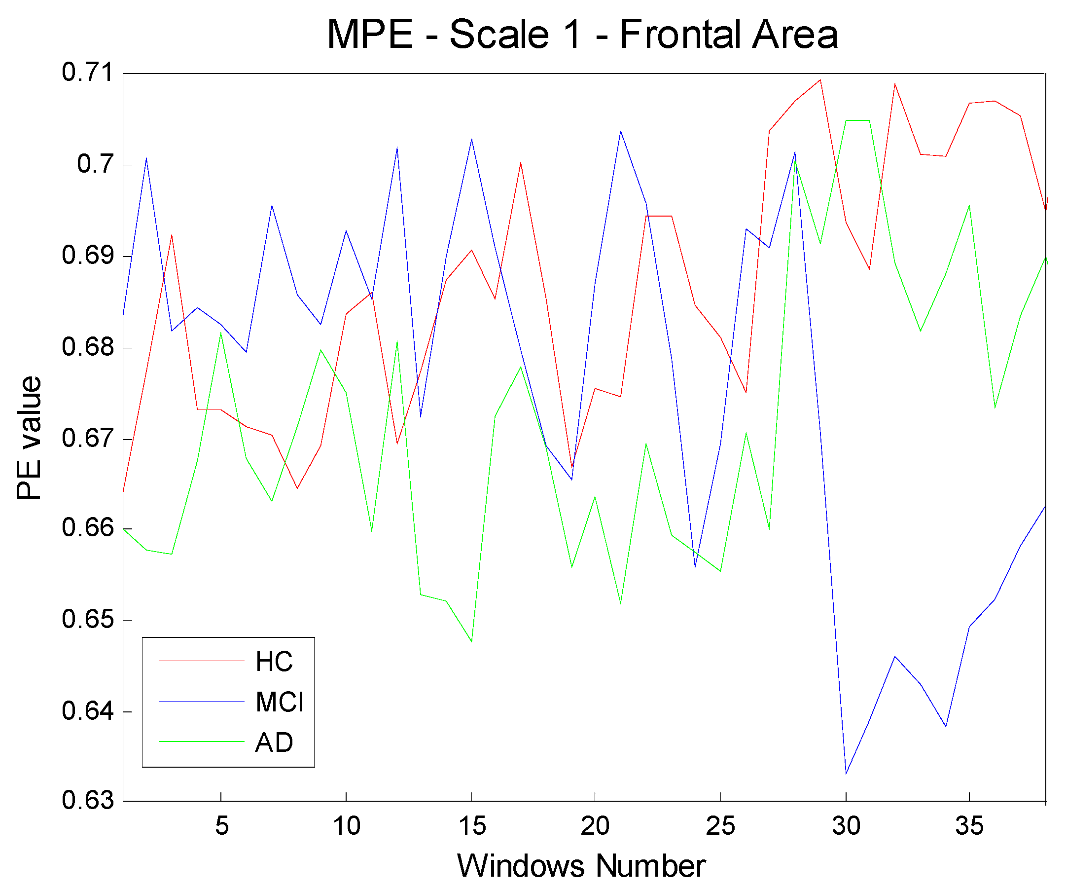
Figure 8 shows an example of the Multivariate Permutation Entropy for the three different categories of subjects. It is clear that, at scale one, the discrimination is difficult at the single window level.
Figure 8.
Multivariate Permutation Entropy for three different categories of subjects: HC (Healthy elderly Control), MCI (Mild Cognitive Impaired patients), and AD (Alzheimer Disease patient). Electrodes (Fp1, Fp2, F3).
Figure 8.
Multivariate Permutation Entropy for three different categories of subjects: HC (Healthy elderly Control), MCI (Mild Cognitive Impaired patients), and AD (Alzheimer Disease patient). Electrodes (Fp1, Fp2, F3).
Figure 9,
Figure 10 and
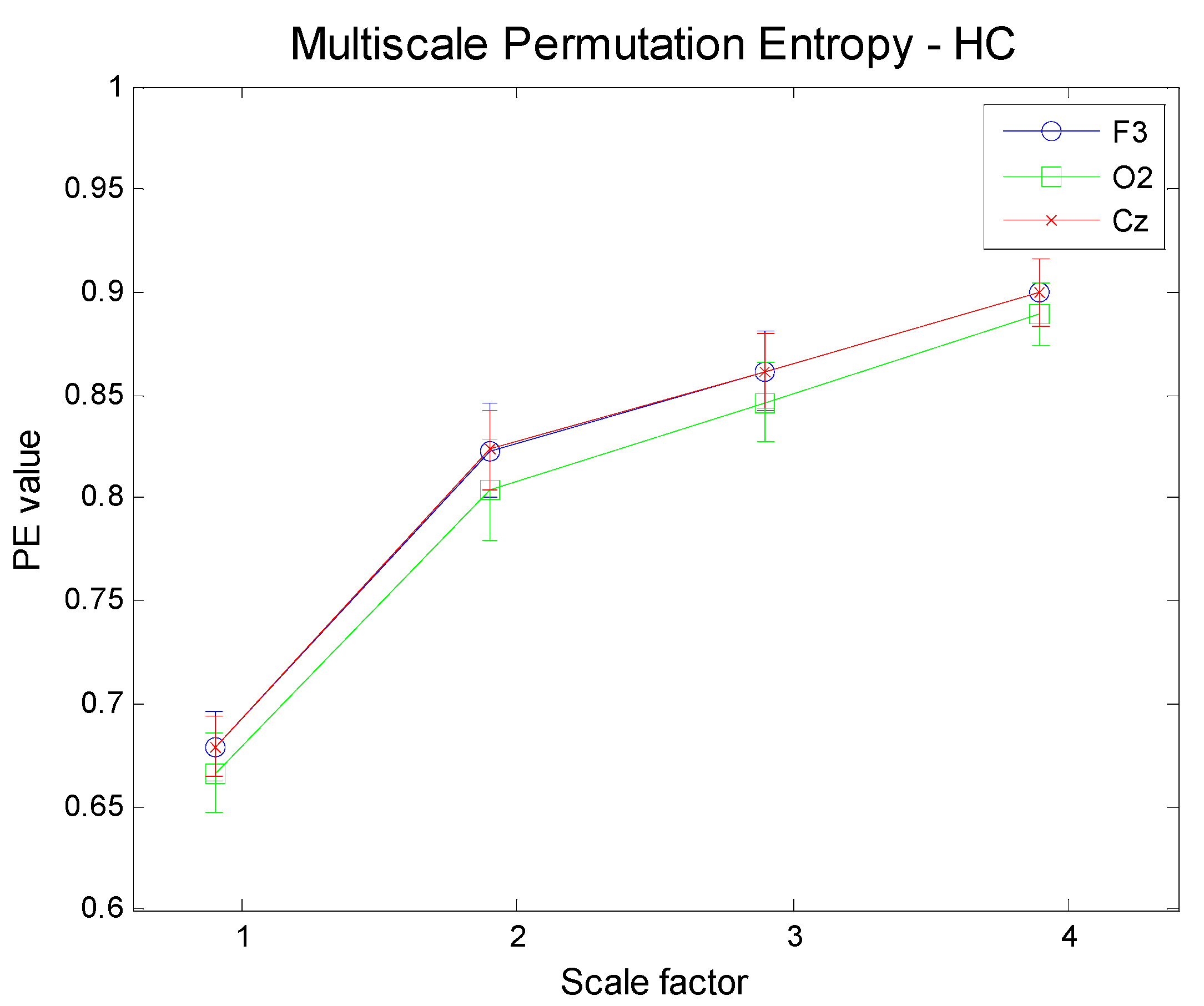
Figure 11 show the results obtained by applying a Multi-Scale analysis to three different electrodes for the three groups. It is worth noting that the complexity increases with scale in any case, in contrast to uncorrelated noise.
Figure 12,
Figure 13 and
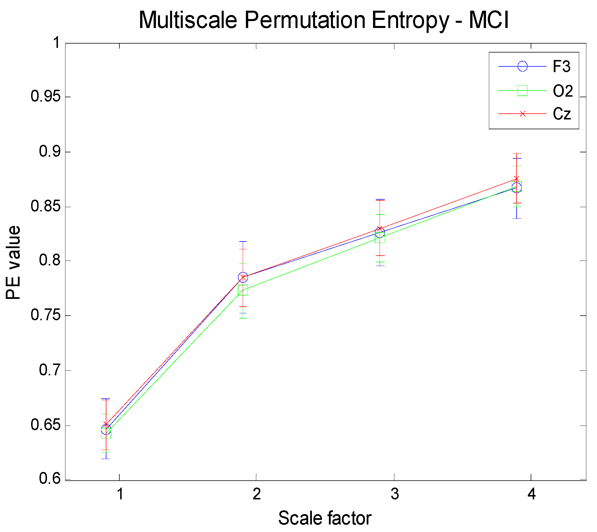
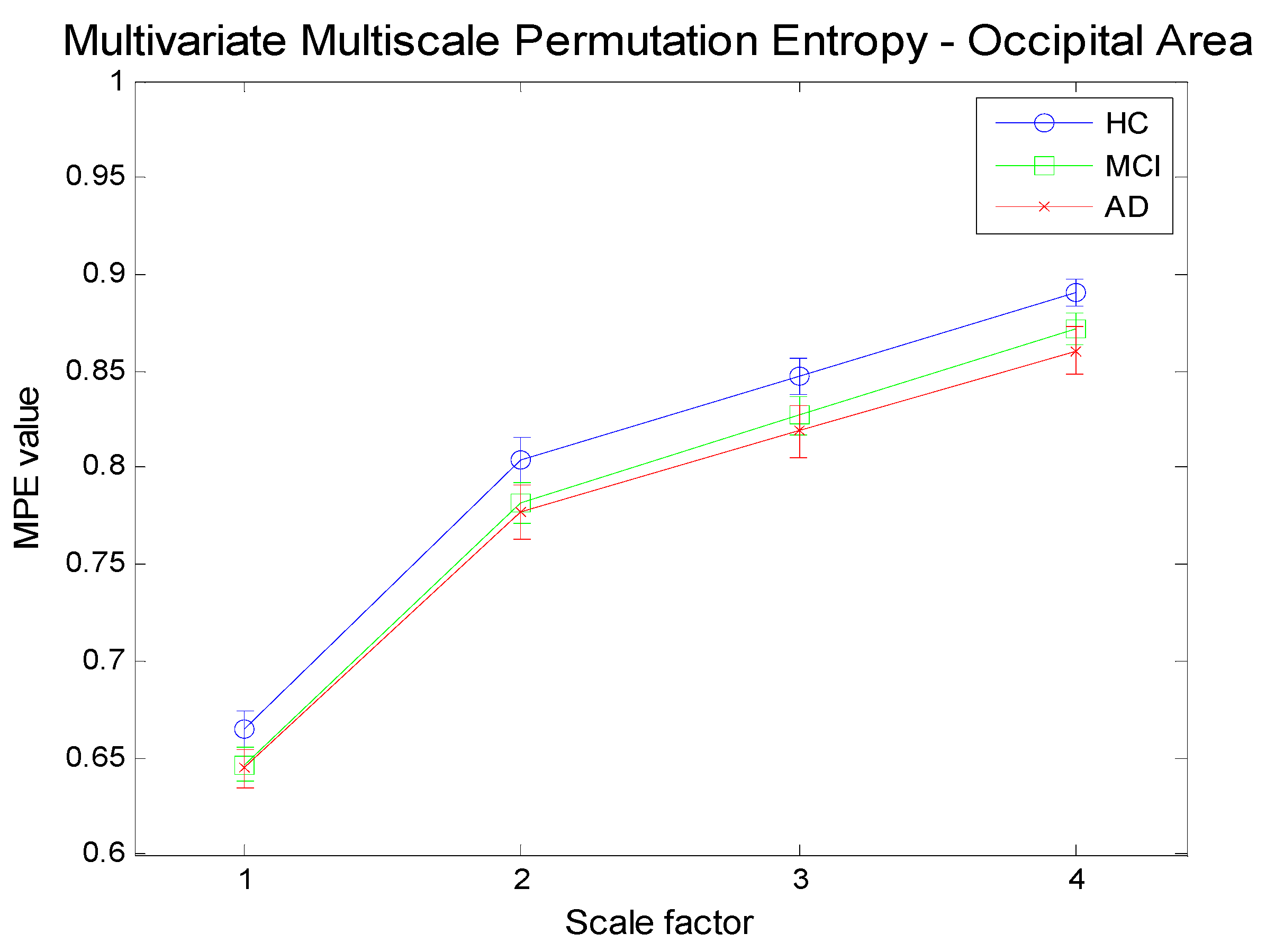
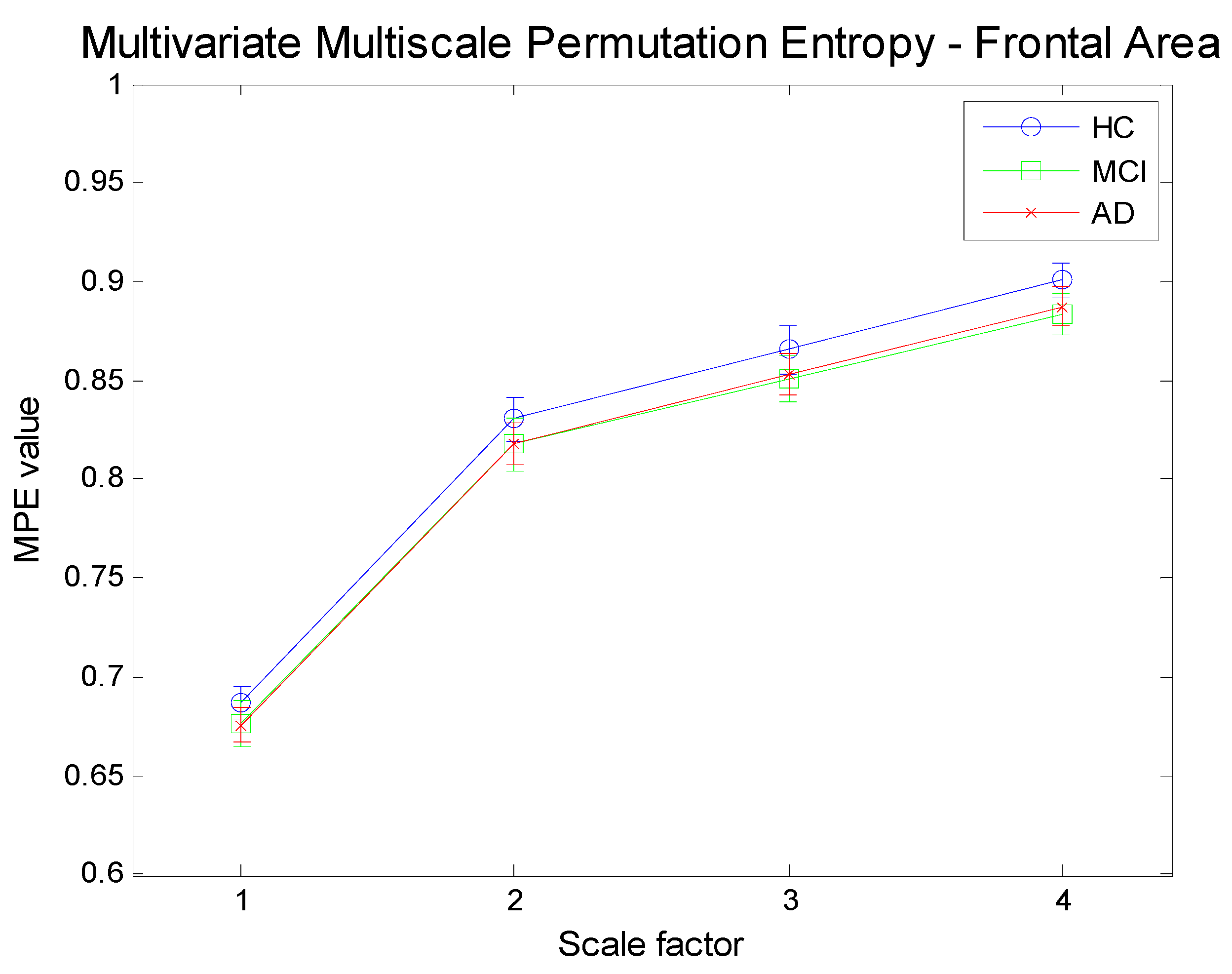
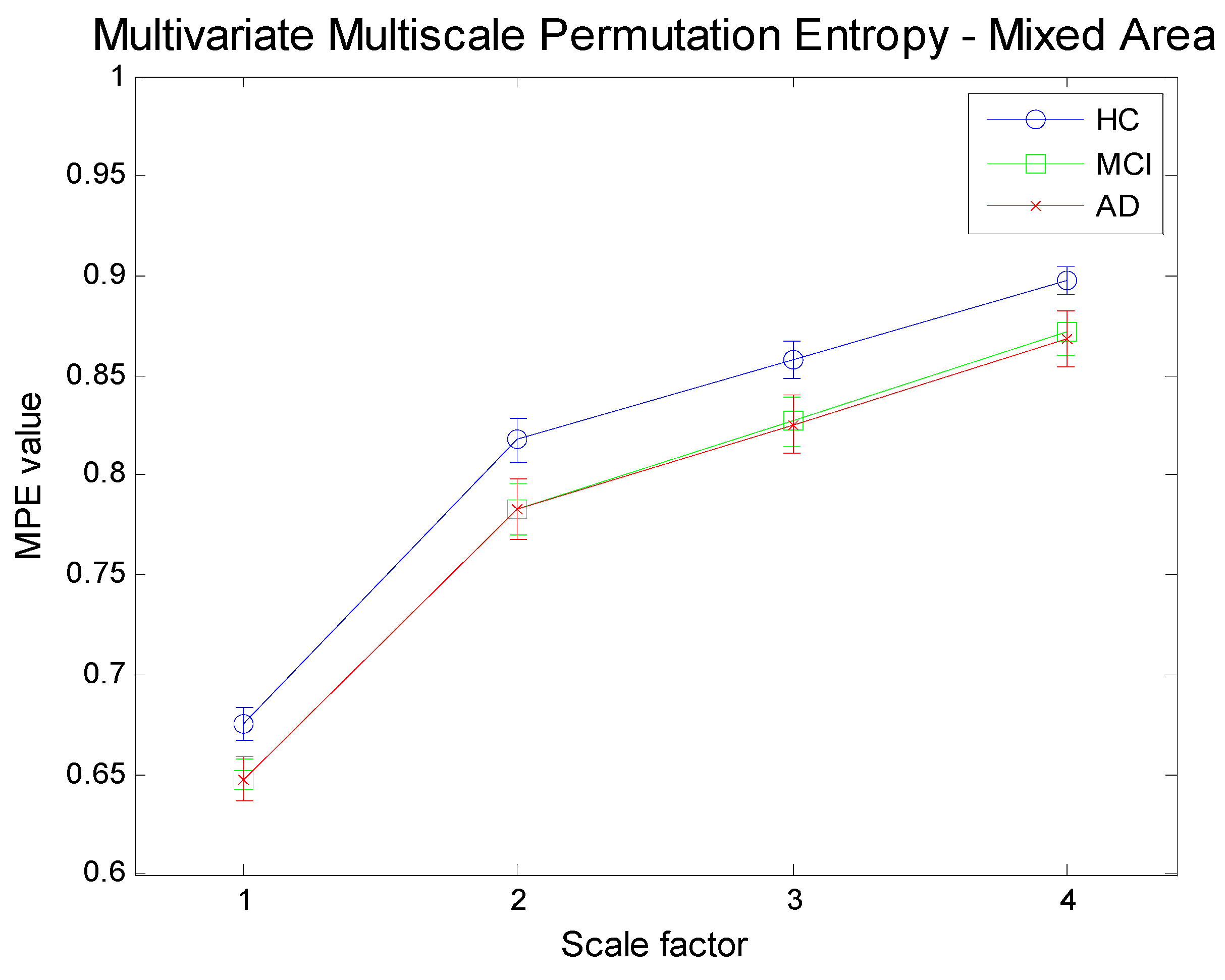
Figure 14 illustrate the results achieved by applying the proposed methodology (MMSPE), with respect to the average values of multivariate PE, at four different scale factors, to the three categories of subjects. Two different brain regions (frontal and occipital electrodes) have been selected along with a different mix of electrodes. Each curve allows for a comparison among complexities, also including the error bars of the estimations. The complexity curves are similar to the ones for the univariate case: AD patients exhibit lower complexity than either MCI or HC subjects and the complexity grows with scale. Since we limited our analysis to scale 4, it is not possible to determine at which scale the curves start to decrease, as reported in other studies [
20,
23,
24]. Unfortunately, because of the limited size of the database, higher scales cannot be tested. One relevant consideration on the MMSPE curves, as compared to univariate MSE, is the sensible reduction of the standard deviation of the complexity estimation. The discrimination between MCI and HC, as well as between AD and HC is quite good and improves with scale. MCI and AD groups are hardly separable. The discrimination among brain states seems more easy when considering electrodes not belonging to the same areas. This appears as a not previously noted advantage of the multivariate approach: in particular, the MMSPE differentiates better from the mere average of the three electrodes MSE curves. In other words, it is possible to hypothesize that in this fictitious “mixed” area, MMSPE helps to capture not trivial correlations. previously noted advantage of multivariate approach areas. to be tested.
Figure 9.
Multi-Scale PE for three different electrodes (F3, frontal; O2, occipital; Cz: central) for normal healthy elderly subjects.
Figure 9.
Multi-Scale PE for three different electrodes (F3, frontal; O2, occipital; Cz: central) for normal healthy elderly subjects.
Figure 10.
Multi-Scale PE for three different electrodes (F3, frontal; O2, occipital; Cz: central) for Mild Cognitive Impaired subjects.
Figure 10.
Multi-Scale PE for three different electrodes (F3, frontal; O2, occipital; Cz: central) for Mild Cognitive Impaired subjects.
Figure 11.
Multi-Scale PE for three different electrodes (F3, frontal; O2, occipital; Cz: central) for subject with Alzheimer’s disease.
Figure 11.
Multi-Scale PE for three different electrodes (F3, frontal; O2, occipital; Cz: central) for subject with Alzheimer’s disease.
Figure 12.
Multivariate Multi-Scale Permutation Entropy (MMSPE) computation for three channels time series referring to the frontal area (Fp1, Fp2, F3) for three different subject categories.
Figure 12.
Multivariate Multi-Scale Permutation Entropy (MMSPE) computation for three channels time series referring to the frontal area (Fp1, Fp2, F3) for three different subject categories.
Figure 13.
Multivariate Multi-Scale Permutation Entropy (MMSPE) computation for three channels time series referring to the occipital area (O1,O2,Oz) for three different subject categories.
Figure 13.
Multivariate Multi-Scale Permutation Entropy (MMSPE) computation for three channels time series referring to the occipital area (O1,O2,Oz) for three different subject categories.
Figure 14.
Multivariate Multi-Scale Permutation Entropy (MMSPE) computation for three channels time series referring to the mixed area (F3,Cz,O2) for three different subject categories.
Figure 14.
Multivariate Multi-Scale Permutation Entropy (MMSPE) computation for three channels time series referring to the mixed area (F3,Cz,O2) for three different subject categories.
