Nonparametric Estimation of Information-Based Measures of Statistical Dispersion

Abstract

We address the problem of non-parametric estimation of the recently proposed measures of statistical dispersion of positive continuous random variables. The measures are based on the concepts of differential entropy and Fisher information and describe the “spread” or “variability” of the random variable from a different point of view than the ubiquitously used concept of standard deviation. The maximum penalized likelihood estimation of the probability density function proposed by Good and Gaskins is applied and a complete methodology of how to estimate the dispersion measures with a single algorithm is presented. We illustrate the approach on three standard statistical models describing neuronal activity.

1. Introduction

Frequently, the dispersion (variability) of measured data needs to be described. Although standard deviation is used ubiquitously for quantification of variability, such approach has limitations. The dispersion of the probability distribution can be understood in different points of view: as “spread” with respect to the expected value, “evenness” (“randomness”) or “smoothness”. For example highly variable data might not be random at all if it consists only of “extremely small” and “extremely large” measurements. Although the probability density function or its estimate provides a complete view, quantitative methods are needed in order to compare different models or experimental results.

In a series of recent studies [1,2] we proposed and justified alternative measures of dispersion. The effort was inspired by various information-based measures of signal regularity or randomness and their interpretations that have gained significant popularity in various branches of science [3,4,5,6,7,8,9]. For convenience, in what follows we discuss only the relative dispersion coefficients (i.e., the data or the probability density function is first normalized to unit mean). Besides the coefficient of variation, $c_v$, which is the relative dispersion measure based on standard deviation, we employ the entropy-based dispersion coefficient $c_h$, and the Fisher information-based coefficient $c_J$. The difference between these coefficients lies in the fact that the Fisher information-based coefficient, $c_J$, describes how “smooth” is the distribution and it is sensitive to the modes of the probability density, while the entropy-based coefficient, $c_h$, describes how “even” it is, hence being sensitive to the overall spread of the probability density over the entire support. Since multimodal densities can be more evenly spread than unimodal ones, the behavior of $c_h$ cannot be generally deduced from $c_J$ (and vice versa).

If a complete description of the data is available, i.e., the probability density function is known, the values of the above mentioned dispersion coefficients can be calculated analytically or numerically. However, the estimation of these coefficients from data is more problematic, and so far we employed either the parametric approach [2] or non-parametric estimation of $c_h$ based on the popular Vasicek’s estimator of differential entropy [10,11]. The goal of this paper is to provide a self-contained method of non-parametric estimation. We describe a method that can be used to estimate both $c_h$ and $c_J$ as a result of a single procedure.

2. Methods

2.1. Dispersion Coefficients

We briefly review the proposed dispersion measures, for more details see [2]. Let T be a continuous positive random variable with probability density function $f\left(t\right)$ defined on $[0,\infty )$. By far, the most common measure of dispersion of T is the standard deviation, σ, defined as the square root of the second central moment of the distribution. The corresponding relative dispersion measure is known as the coefficient of variation, $c_v$,

$$c_v=\frac{\sigma }{\mathrm{E}\left(T\right)}$$

(1)

where $\mathrm{E}\left(T\right)$ is the mean value of T.

The entropy-based dispersion coefficient is defined as

$$c_h=\frac{exp\left[h\right(T)-1]}{\mathrm{E}\left(T\right)}$$

(2)

where $h\left(T\right)$ is the differential entropy [12],

$$h\left(T\right)=-\underset{0}{\overset{\infty }{\int }}f\left(t\right)lnf\left(t\right)dt$$

(3)

The numerator in (2), ${\sigma }_h=exp[h\left(T\right)-1]$, is the entropy-based dispersion, “analogous” to the notion of standard deviation σ. The interpretation of ${\sigma }_h$ relies on the asymptotic equipartition property theorem [12]. Informally, the theorem states that almost any sequence of n realizations of the random variable T comes from a rather small subset (the typical set) in the n-dimensional space of all possible values. The volume of this subset is approximately ${\sigma }_h^n=exp\left[nh\left(T\right)\right]$, and the volume is bigger for those random variables, which generate more diverse (or unpredictable) realizations. The values of ${\sigma }_h$ and $c_h$ quantify how “evenly” is the probability distributed over the entire support. From this point of view, ${\sigma }_h$ is more appropriate than σ to describe the randomness of outcomes generated by the random variable T.

The Fisher information-based dispersion coefficient, $c_J$, is defined as

$$c_J=\frac{1}{\mathrm{E}\left(T\right)\sqrt{J\left(T\right)}}$$

(4)

where

$$\begin{array}{c}\hfill J\left(T\right)=\underset{0}{\overset{\infty }{\int }}{\left[\frac{\partial lnf\left(t\right)}{\partial t}\right]}^{2}f\left(t\right)dt\end{array}$$

(5)

The Fisher information is traditionally interpreted by means of the Cramer–Rao bound, i.e., the value of $1/J\left(T\right)$ is the lower bound on the error of any unbiased estimator of a location parameter of the distribution. Due to the derivative in (5), certain regularity conditions are required on $f\left(t\right)$ in order for $J\left(T\right)$ to be interpreted according to the Cramer–Rao bound, namely continuous differentiability for all $t>0$ and $f\left(0\right)=f^{\prime }\left(0\right)=0$, [13]. However, the integral in (5) exists and is finite also for, e.g., an exponential distribution. Any locally steep slope or the presence of modes in the shape of $f\left(t\right)$ increases $J\left(T\right)$, [4].

2.2. Methods of Non-Parametric Estimation

In the following we assume that $\{t_1,t_2,\dots ,t_N\}$ are N independent realizations of the random variable $T\sim f\left(t\right)$, defined on $[0,\infty )$.

The $c_v$ is most often estimated by the ratio of sample standard deviation to sample mean, however, the estimate may be considerably biased, [14].

Estimation of $c_h$ relies on the estimate $\widehat{h}$ of the differential entropy $h\left(T\right)$, as follows from (2). The problem of differential entropy estimation is well exploited in literature [11,15,16]. It is preferable to avoid estimations based on data binning (histograms), because discretization affects the results. The most popular approaches are represented by the class of Kozachenko–Leonenko estimators [17,18] and the Vasicek’s estimator [10]. Our experience shows that the simple Vasicek’s estimator gives good results on a wide range of data [19,20,21], thus in this paper we employ it for the sake of comparison with the estimation method described further below. Given the ranked observations $t_{\left[1\right]}<t_{\left[2\right]}<\cdots <t_{\left[N\right]}$, the Vasicek’s estimator $\widehat{h}$ is defined as

$$\widehat{h}=\frac{1}{N}\sum _{i=1}^{N}ln\left(t_{[i+m]}-t_{[i-m]}\right)+ln\frac{N}{2m}+{\phi }_{\mathrm{bias}}$$

(6)

where $t_{[i+m]}=t_{\left[m\right]}$ for $i+m>N$ and $t_{[i-m]}=t_{\left[1\right]}$ for $i-m<1$. The integer parameter $m<N/2$ is set prior to the calculation, roughly one may set m to be the integer part of $\sqrt{N}$. The bias-correcting factor is

$${\phi }_{\mathrm{bias}}=ln\frac{2m}{N}+\left(1-\frac{2m}{N}\right)\Psi \left(2m\right)+\Psi (N+1)-\frac{2}{N}\sum _{i=1}^m\Psi (i+m-1)$$

(7)

where $\Psi \left(z\right)=\frac{d}{dz}ln\Gamma \left(z\right)$ denotes the digamma function, [22].

The estimation of $c_J$ requires estimation of $J\left(T\right)$, and it is more problematic and as far as we know no “standard” algorithms have been proposed.

Huber [23] showed that there exists a unique interpolation of the empirical cumulative distribution function such that the resulting Fisher information is maximized. In theory, one may use this method to estimate $J\left(T\right)$. Unfortunately, it is very complicated and probably not feasible even for moderate values of N.

Kernel density estimators are widely used for estimation of the density. They can be successfully used for the calculation of the differential entropy too [24,25]. But, according to our experience, they are unsuitable for estimation of the Fisher information, mainly due to the inability to control the “smoothness” of the ratio $f^{\prime }/f$, which is the principal term in the integral (5). Inappropriate choice of the kernel and the bandwidth leads to many local extremes of the kernel density estimator which substantially increases the Fisher information. Theoretically, the kernel should be “optimal” in the sense of minimizing the mean square error of the ratio $f^{\prime }/f$, which is difficult to derive in a closed form, generally. One may also derive Vasicek-like estimator of $J\left(T\right)$, based on the empirical cumulative distribution function and considering differences of higher order, however, we discovered that this approach is numerically unstable.

We found that the maximum penalized likelihood (MPL) method of Good and Gaskins [26] for probability density estimation offers a possible solution. The idea is to represent the whole probability density function using a suitable orthogonal base of functions (Hermite functions), and the “best” estimate of $f\left(t\right)$ is obtained by solving a set of equations for the base coefficients given the sample $\{t_1,\dots ,t_N\}$.

In order to proceed, we first log-transform and normalize the sample,

$$x_i=\frac{ln{t}_i-\mu }{\sqrt{2{\sigma }^2}}$$

(8)

where

$$\mu =\frac{1}{N}\sum _{i=1}^{N}ln{t}_i\mathrm{and}{\sigma }^2=\frac{1}{N-1}\sum _{i=1}^N{\left(ln{t}_i-\mu \right)}^2$$

(9)

The idea here is to obtain a new random variable X, $X=(lnT-\mu )/\sqrt{2{\sigma }^2}$, with a more Gaussian-like density shape unlike the shape of the distribution of T, which is usually highly skewed. Furthermore, the limitation of the support of T to the real half-line may cause numerical difficulties. The probability density function of X is expressed by the real probability amplitude $c\left(x\right)$, so that $X\sim c^2\left(x\right)$. For the purpose of numerical implementation, $c\left(x\right)$ is represented by the first r Hermite functions, [22], as

$$c\left(x\right)=\sum _{m=0}^{r-1}{c}_m{\psi }_m\left(x\right)$$

(10)

where

$${\psi }_m\left(x\right)={\left[\sqrt{\pi }{2}^{m}m!\right]}^{-1/2}exp\left(-x^2/2\right)H_m\left(x\right)$$

(11)

and $H_m\left(x\right)$ denotes the Hermite polynomial $H_m\left(x\right)={(-1)}^{m}exp\left(x^2\right)\frac{d^m}{d{x}^m}exp\left(-x^2\right)$.

The goal is to find such $c=c\left(x\right)$, for which the score, ω, is maximized,

$$\omega (c;x_1,\dots ,x_N)=l(c;x_1,\dots ,x_N)-\Phi \left(c\right)$$

(12)

subject to constraint (ensuring that $c^2\left(x\right)$ is a probability density function)

$$\sum _{m=0}^{r-1}{c}_m^2=1$$

(13)

The term $l(c;x_1,\dots ,x_N)$ in (12) is the log-likelihood function,

$$l(c;x_1,\dots ,x_N)=2\sum _{i=1}^{N}lnc\left(x_i\right)$$

(14)

and Φ is the roughness penalty proposed by [26], controlling the smoothness of the density of X (and hence the smoothness of $f\left(t\right)$),

$$\Phi (c;\alpha ,\beta )=4\alpha {\int }_{-\infty }^{\infty }{c}^{\prime }{\left(x\right)}^{2}dx+\beta {\int }_{-\infty }^{\infty }{c}^{\prime \prime }{\left(x\right)}^{2}dx$$

(15)

The two nonnegative parameters α and β ( $\alpha +\beta >0$) should be set prior to the calculation. Note that the first term in (15) is equal to α-times the Fisher information $J\left(X\right)$.

The system of equations for $c_i$’s which maximize (12) can be written as [26]

$$\begin{array}{cc}\hfill \frac{1}{2}\beta \sqrt{k(k-1)(k-2)(k-3)}{c}_{k-4}& -\sqrt{k(k-1)}\left[4\alpha +(2k-1)\beta \right]c_{k-2}+\hfill \\ \hfill +\left[2\lambda +8\alpha k+\beta k(k+1)\right]c_k& -\sqrt{(k+1)(k+2)}\left[4\alpha +(2k+3)\beta \right]c_{k+2}+\hfill \\ \hfill +\frac{1}{2}\beta \sqrt{(k+1)(k+2)(k+3)(k+4)}{c}_{k+4}& =2\sum _{i=1}^N\frac{{\psi }_k\left(x_i\right)}{{\sum }_{m=0}^{r-1}{c}_m{\psi }_m\left(x_i\right)}\hfill \end{array}$$

(16)

for $k=0,1,\dots ,r-1$. The system can be solved iteratively as follows. Initially $c_0=1$, $c_m=0$ for $m=1,2,\dots$ and $\lambda =N$, which gives the approximation of X by a Gaussian random variable. Then, in each iteration step, current values of $c_0,\dots ,c_{r-1}$ are substituted into the right hand side of (16), and the system is solved as a linear system with unknown variables $c_0,\dots ,c_{r-1}$ appearing on the left hand side of (16). Once the linear system is solved, the coefficients are normalized to satisfy (13). The corresponding Lagrange multiplier is calculated as

$$\begin{array}{cc}\hfill \lambda & =N+\alpha \left\{2-4\sum _{m=0}^{r-1}\left[\left(m+\frac{1}{2}\right)c_m^2-\sqrt{(m+1)(m+2)}{c}_m{c}_{m+2}\right]\right\}+\hfill \\ \hfill & +\beta \left\{\frac{3}{4}-\sum _{m=0}^{r-1}\left[\frac{3}{4}(2m^2+2m+1)c_m^2-(2m+3)\sqrt{(m+1)(m+2)}{c}_m{c}_{m+2}+\right.\right.\hfill \\ & \left.\left.+\frac{1}{2}\sqrt{(m+1)(m+2)(m+3)(m+4)}{c}_m{c}_{m+4}\right]\right\}\hfill \end{array}$$

(17)

The $r+1$ variables (r coefficients and the Lagrange multiplier λ) are computed iteratively. In accordance with [26], the algorithm is stopped when λ does not change within desired precision in subsequent iterations.

After the score-maximizing $c_i$’s are obtained, and thus the density of X is estimated, the estimates of dispersion coefficients in (2) and (4) are calculated from the following entropy and Fisher information estimators. The change of variables gives

$$\widehat{h\left(T\right)}=\widehat{h\left(X\right)}+\mu +ln\left(\sqrt{2}\sigma \right)+\sqrt{2}\sigma \widehat{\mathrm{E}\left(X\right)}$$

(18)

where $\widehat{h\left(X\right)}=-2{\int }_{-\infty }^{\infty }c{\left(x\right)}^{2}ln\left|c\left(x\right)\right|dx$ is the estimator of the differential entropy of X, μ and σ are given by (9) and $\widehat{\mathrm{E}\left(X\right)}={\int }_{-\infty }^{\infty }xc{\left(x\right)}^{2}dx$ is the estimated expected value of X. (Numerically, $\widehat{E\left(X\right)}$ is usually small and can be neglected. Its value is influenced by the number, r, of considered Hermite functions.)

The Fisher information estimator then follows, by an analogous change of variables, as

$$\widehat{J\left(T\right)}=\frac{exp(-2\mu )}{{\sigma }^2}{\int }_{-\infty }^{\infty }{\left[\sqrt{2}{c}^{\prime }\left(x\right)-\sigma c\left(x\right)\right]}^{2}exp\left(-2\sqrt{2}\sigma x\right)dx$$

(19)

The calculation requires the first derivative of $c\left(x\right)$ [22],

$$c^{\prime }\left(x\right)=\frac{1}{\sqrt{2}}\sum _{m=1}^{r-1}{c}_m\sqrt{m}{\psi }_{m-1}\left(x\right)-\frac{1}{\sqrt{2}}\sum _{m=0}^{r-1}{c}_m\sqrt{m+1}{\psi }_{m+1}\left(x\right)$$

(20)

3. Results

Neurons communicate via the process of synaptic transmission, which is triggered by an electrical discharge called the action potential or spike. Since the time intervals between individual spikes are relatively large when compared to the spike duration, and since for any particular neuron the “shape” or character of a spike remains constant, the spikes are usually treated as point events in time. Spike train consists of times of spike occurrences ${\tau }_0,{\tau }_1,\cdots ,{\tau }_n$, equivalently described by a set of n interspike intervals (ISIs) $t_i={\tau }_i-{\tau }_{i-1}$, $i=1\cdots n$, and these ISIs are treated as independent realizations of the random variable $T\sim f\left(t\right)$. The probabilistic description of the spiking results from the fact that the positions of spikes cannot be predicted deterministically due to presence of intrinsic noise, only the probability that a spike occurs can be given [27,28,29]. In real neuronal data, however, the non-renewal property of the spike trains is often observed [30,31]. Taking the serial correlation of the ISIs as well as any other statistical dependence into account would result in the decrease of the entropy and hence of the value of $c_h$, see [12].

We compare exact and estimated values of the dispersion coefficients on three widely used statistical models of ISIs: gamma, inverse Gaussian and lognormal. Since only the relative coefficients are discussed, $c_v,c_h,c_J$, we parameterize each distributions by its $c_v$ while keeping $E\left(T\right)=1$.

The gamma distribution is one of the most frequent statistical descriptors of ISIs used in analysis of experimental data [32]. Probability density function of gamma distribution can be written as

$$f_{\Gamma }\left(t\right)={\left(c_v^2\right)}^{-1/c_v^2}{\left[\Gamma \left(1/c_v^2\right)\right]}^{-1}{t}^{1/c_v^2-1}exp\left(-t/c_v^2\right)$$

(21)

where $\Gamma \left(z\right)={\int }_0^{\infty }{t}^{z-1}exp(-t)dt$ is the gamma function, [22]. The differential entropy is equal to, [2],

$$h_{\Gamma }=\frac{1}{c_v^2}+ln{c}_v^2+ln\Gamma \left(\frac{1}{c_v^2}\right)+\left(1-\frac{1}{c_v^2}\right)\Psi \left(\frac{1}{c_v^2}\right)$$

(22)

where $\Psi \left(z\right)=\frac{d}{dz}ln\Gamma \left(z\right)$ denotes the digamma function, [22]. The Fisher information about the location parameter is

$$J_{\Gamma }=\frac{1}{c_v^2(1-2c_v^2)}for0<c_v<\frac{1}{\sqrt{2}}$$

(23)

The Fisher information diverges for $c_v\ge 1/\sqrt{2}$, with the exception of $c_v=1$ (corresponds to exponential distribution) where $J_{\Gamma }=1$, but the Cramer–Rao based interpretation of $J_{\Gamma }$ does not hold in this case since $f_{\Gamma }\left(0\right)\ne 0$, see [13] for details.

The inverse Gaussian distribution is often used for description of ISIs and fitted to experimental data. It arises as result of spiking activity of a stochastic variant of the perfect integrate-and-fire neuronal model [33]. The density of this distribution is

$$f_{\mathrm{IG}}\left(t\right)=\sqrt{\frac{1}{2\pi c_v^2{t}^3}}exp\left[-\frac{{(t-1)}^2}{2c_v^{2}t}\right]$$

(24)

The differential entropy of this distribution is equal to

$$h_{\mathrm{IG}}=\frac{ln\left(2\pi e{c}_v^2\right)}{2}-\frac{3}{\sqrt{2\pi c_v^2}}exp\left(c_v^{-2}\right)K^{(1,0)}\left(\frac{1}{2},c_v^{-2}\right)$$

(25)

where $K^{(1,0)}(\nu ,z)$ denotes the first derivative of the modified Bessel function of the second kind [22], $K^{(1,0)}(\nu ,z)=\frac{d}{d\nu }K(\nu ,z)$. The Fisher information of the inverse Gaussian distribution results in

$$J_{\mathrm{IG}}=\frac{21c_v^6+21c_v^4+9c_v^2+2}{2c_v^2}$$

(26)

The lognormal distribution is rarely presented as model distribution of ISIs. However, it represents a common descriptor in analysis of experimental data [33], with density

$$f_{\mathrm{LN}}\left(t\right)=\sqrt{\frac{1}{2\pi tln(1+c_v^2)}}exp\left\{-\frac{{[ln(1+c_v^2)+ln{t}^2]}^2}{8ln(1+c_v^2)}\right\}$$

(27)

The differential entropy of this distribution is equal to

$$h_{\mathrm{LN}}=ln\sqrt{2\pi e\frac{ln(1+c_v^2)}{1+c_v^2}}$$

(28)

and the Fisher information is given by

$$J_{\mathrm{LN}}=\frac{{(1+c_v^2)}^3[1+ln(1+c_v^2)]}{ln(1+c_v^2)}$$

(29)

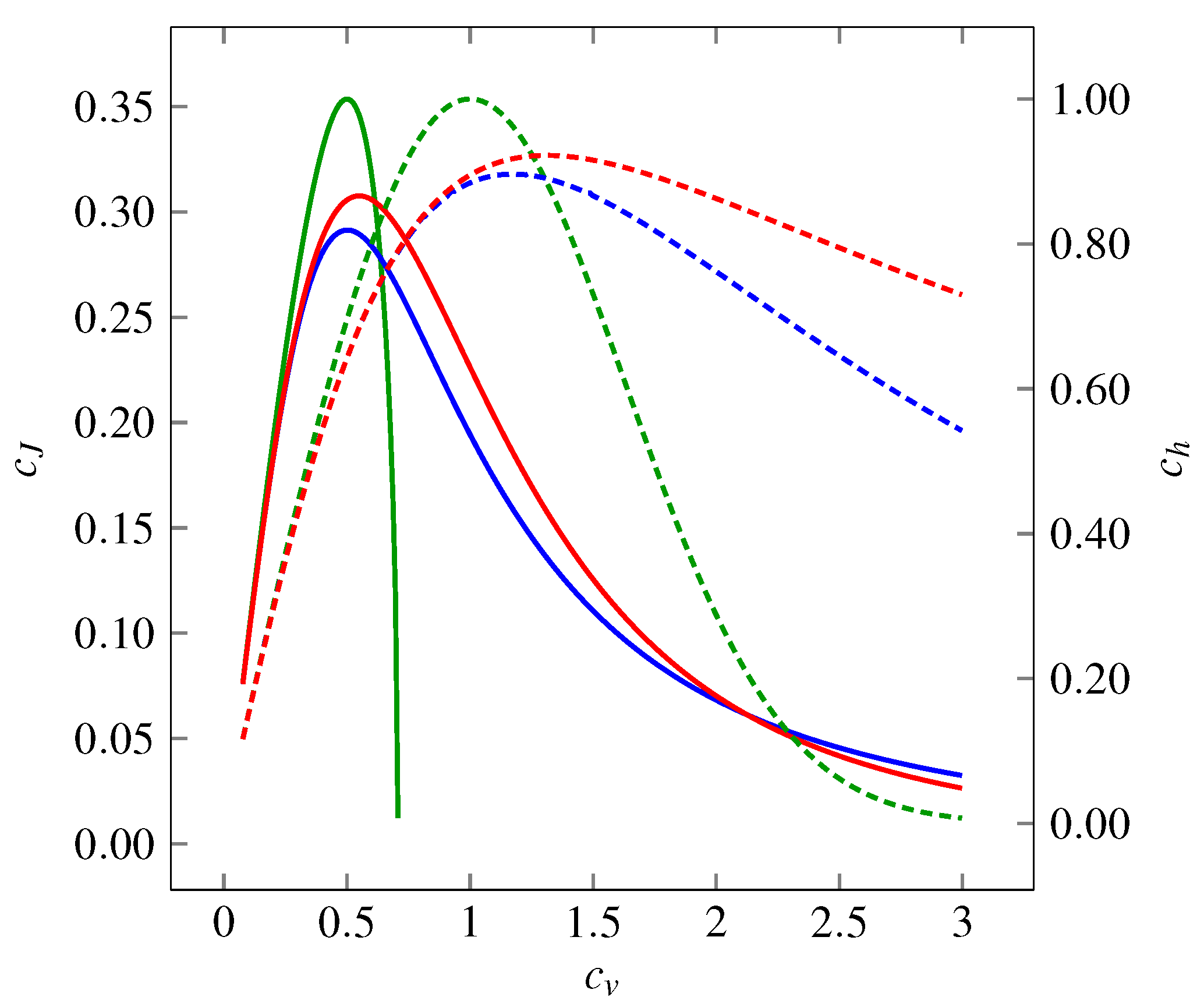
The theoretical values of the coefficients of $c_h$ and $c_J$ as functions of $c_v$ are shown in Figure 1 for all the three distributions mentioned above. We see that the functions form hill-shaped curves with local maxima achieved for different values of $c_v$. Asymptotically, $c_h$ as well as $c_J$ tend to zero for $c_v\to 0$ or $c_v\to \infty$ for the three models.

Figure 1. Variability represented by the coefficient of variation $c_v$, the entropy-based coefficient $c_h$ (dashed curves, right-hand-side axis) and the Fisher information-based coefficient $c_J$ (solid curves, left-hand-side axis) of three probability distributions: gamma (green curves), inverse Gaussian (blue curves) and lognormal (red curves). The entropy-based coefficient, $c_h$, expresses the evenness of the distribution. In dependency on $c_v$, it shows a maximum at $c_v=1$ for gamma distribution (corresponds to exponential distribution) and between $c_v=1$ and $c_v=1.5$ for inverse Gaussian and lognormal distributions. For all the distributions holds $c_h\to 0$ as $c_v\to 0$ or $c_v\to \infty$. The Fisher information-based coefficient, $c_J$, grows as the distributions become “smoother”. The overall dependence on $c_v$ shows a maximum around $c_v=0.5$. Similarly to $c_h\left(c_v\right)$ dependencies, $c_h\to 0$ as $c_v\to 0$ or $c_v\to \infty$ (does not hold for gamma distribution, where $c_J$ can be calculated only for $c_v<1/\sqrt{2}$).

Figure 1. Variability represented by the coefficient of variation $c_v$, the entropy-based coefficient $c_h$ (dashed curves, right-hand-side axis) and the Fisher information-based coefficient $c_J$ (solid curves, left-hand-side axis) of three probability distributions: gamma (green curves), inverse Gaussian (blue curves) and lognormal (red curves). The entropy-based coefficient, $c_h$, expresses the evenness of the distribution. In dependency on $c_v$, it shows a maximum at $c_v=1$ for gamma distribution (corresponds to exponential distribution) and between $c_v=1$ and $c_v=1.5$ for inverse Gaussian and lognormal distributions. For all the distributions holds $c_h\to 0$ as $c_v\to 0$ or $c_v\to \infty$. The Fisher information-based coefficient, $c_J$, grows as the distributions become “smoother”. The overall dependence on $c_v$ shows a maximum around $c_v=0.5$. Similarly to $c_h\left(c_v\right)$ dependencies, $c_h\to 0$ as $c_v\to 0$ or $c_v\to \infty$ (does not hold for gamma distribution, where $c_J$ can be calculated only for $c_v<1/\sqrt{2}$).

To explore the accuracy of the estimators of the coefficients $c_h$ and $c_J$ when the MPL estimations of the densities are employed, we did three separate simulation studies. All the simulations and calculations were performed in the free software package R [34]. For each model with the probability distribution (21), (24) and (27), respectively, the coefficient of variation, $c_v$, varied from $0.1$ to $3.0$ in steps of $0.1$. One thousand samples, each consisting of 1000 random numbers (a common number of events in experimental records of neuronal firing), were taken for each value of $c_v$ from the three distributions.

The MPL method was employed on each generated sample to estimate the density. We chose the number of the base functions equal to $r=20$. The larger bases, $r=50$ or $r=100$, were examined too, with negligible differences in the estimation for the selected models. The values of the parameters for (15) were chosen as $\alpha =3$ and $\beta =4$, in accordance with the suggestion ([26], Appendix A).

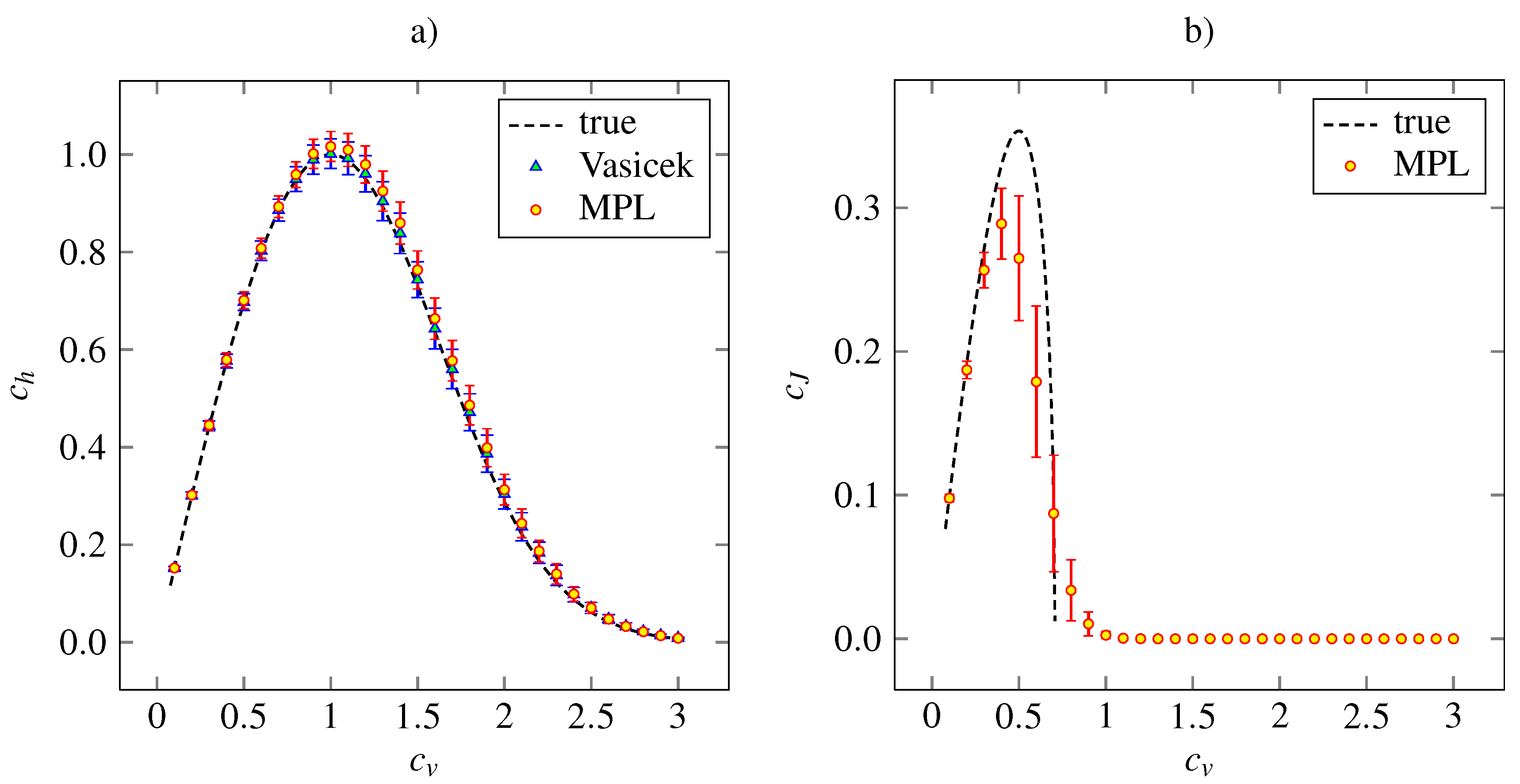
The outcome of the simulation study for the gamma density (21) is presented in Figure 2, where the theoretical and estimated values of $c_h$ and $c_J$ for given $c_v$ are plotted. In addition, the values of coefficient $c_h$ calculated by Vasicek’s estimator are shown. We see that the MPL method results in precise estimation of $c_h$ for low values of $c_v$ and in slightly overestimated values of $c_h$ for $c_v>0.7$. The Vasicek’s estimator gives slightly overestimated values too. Overall, the performances of Vasicek’s and MPL estimators are comparable. The maximum of the MPL estimator of $c_h$ is achieved at the theoretical value, $c_v=1$. We can see that the standard deviation of the $c_h$ estimate is higher as $c_v$ grows from zero. As $c_v>1$, the standard deviation begins to decrease slowly.

We conclude that the MPL estimator of $c_J$ is accurate for low $c_v$. For $c_v>0.5$ it results in underestimated $c_J$ and it tends to zero as $c_v\to 1/\sqrt{2}$ as well as the theoretical values. The high bias of $c_J$ for high $c_v$ is caused by inappropriate choice of the parameters α and β, which were kept fixed in accordance with the suggestion of [26]. Nevertheless, the main shape of the dependency on $c_v$ remains and the MPL estimates of $c_J$ achieves local maximum at $c_v\doteq 0.55$, which is slightly lower than the theoretical value.

Figure 2. The entropy-based variability coefficient $c_h$ (panel a) and the Fisher information-based variability coefficient $c_J$ (panel b), calculated nonparametrically from (18) and (19), respectively, for gamma distribution (24). The mean values (indicated by red discs) accompanied by the standard error (red error bars) are plotted in dependency on the coefficient of variation, $c_v$. The dashed lines are the theoretical curves. In panel a, the results obtained by estimation (6) are added (blue triangles indicate mean values and blue error bars stand for standard error). The results are based on 1000 trials of samples of size 1000 for each value of $c_v$.

Figure 2. The entropy-based variability coefficient $c_h$ (panel a) and the Fisher information-based variability coefficient $c_J$ (panel b), calculated nonparametrically from (18) and (19), respectively, for gamma distribution (24). The mean values (indicated by red discs) accompanied by the standard error (red error bars) are plotted in dependency on the coefficient of variation, $c_v$. The dashed lines are the theoretical curves. In panel a, the results obtained by estimation (6) are added (blue triangles indicate mean values and blue error bars stand for standard error). The results are based on 1000 trials of samples of size 1000 for each value of $c_v$.

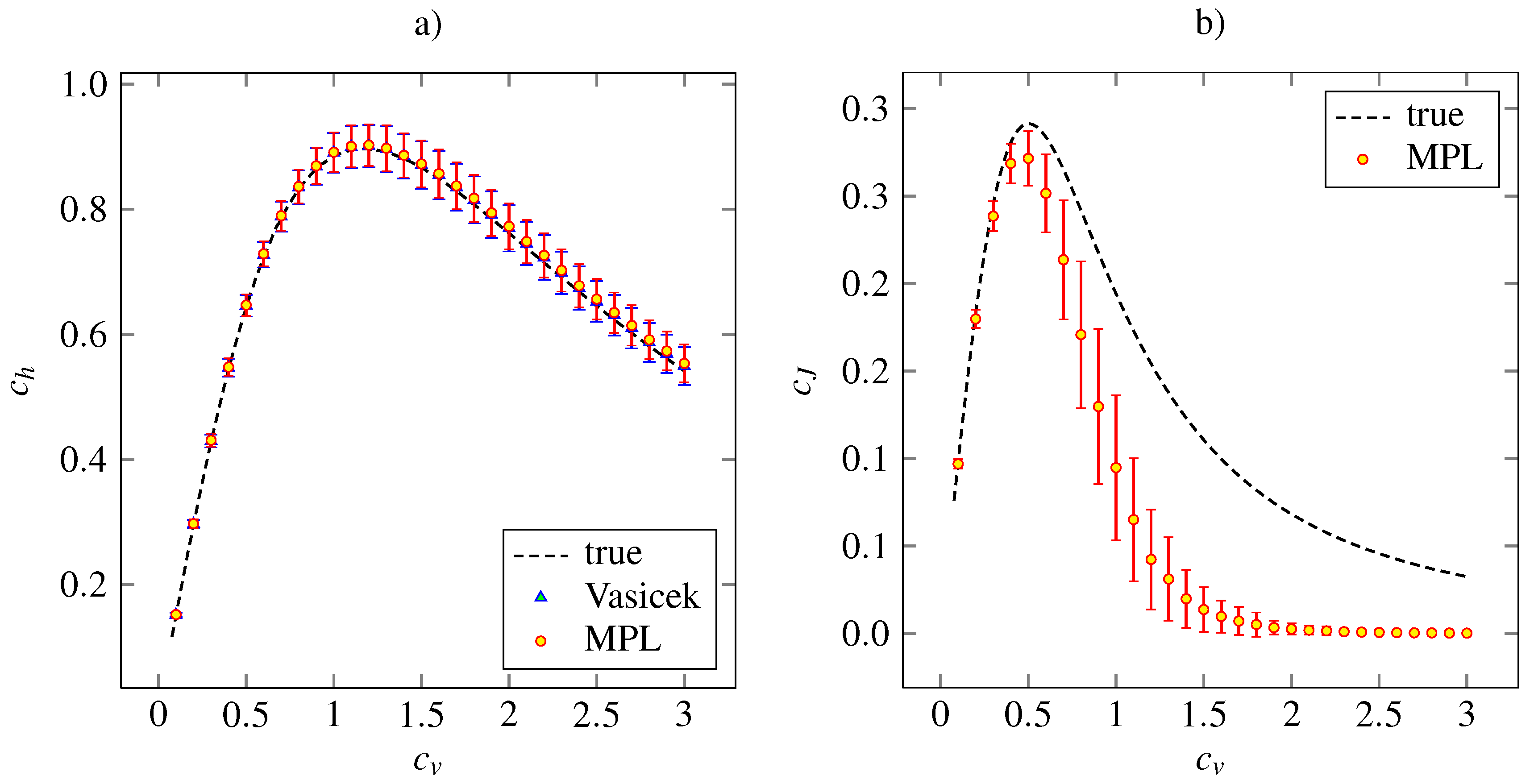
Figure 3 shows the corresponding results for the inverse Gaussian density. The Vasicek’s and MPL estimates of $c_h$ are almost precise. Both the estimator of $c_h$ based on MPL method and that based on the Vasicek’s entropy give the same mean values together with the same standard deviations. The MPL estimator of $c_J$ gives accurate and precise results for $c_v<0.5$. For higher $c_v$, the estimated value is lower than the true one. The maximum of estimated $c_J$ is achieved at the same point, $c_v\doteq 0.5$. The asymptotical decrease of the estimated $c_J$ to zero is faster than the true dependency is. By our experience, this can be improved by setting higher α and β in order to give higher impact to the roughness penalty (15).

Figure 3. Estimations of the variability coefficients $c_h$ (panel a) and $c_J$ (panel b) for inverse Gaussian distribution (24). The notation and the layout is the same as in Figure 2.

Figure 3. Estimations of the variability coefficients $c_h$ (panel a) and $c_J$ (panel b) for inverse Gaussian distribution (24). The notation and the layout is the same as in Figure 2.

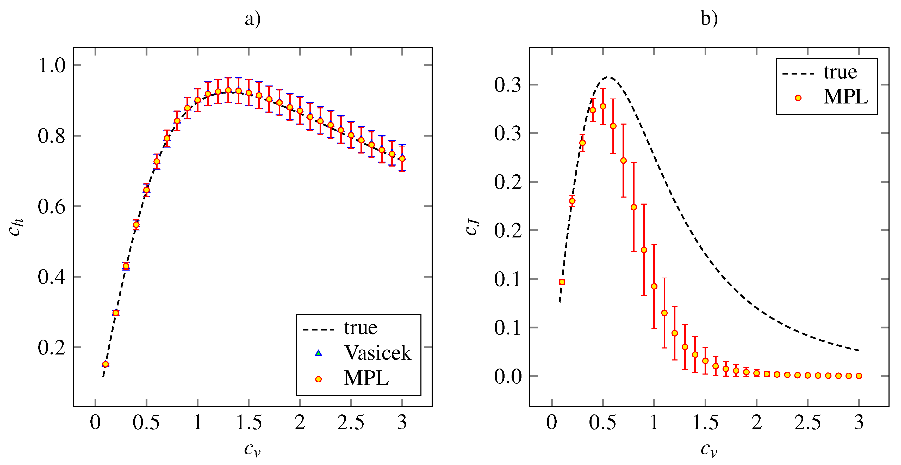
The results of the simulation study on the lognormal distribution with density (27) is plotted in Figure 4, together with the theoretical dependencies and the results for the Vasicek’s estimator of the entropy. Both the MPL estimators of $c_h$ and $c_J$ have qualitatively same accuracy and precision features as the analogous estimators for the inverse Gaussian model.

Figure 4. Estimations of the variability coefficients $c_h$ (panel a) and $c_J$ (panel b) for lognormal distribution (27). The notation and the layout is the same as in Figure 2.

Figure 4. Estimations of the variability coefficients $c_h$ (panel a) and $c_J$ (panel b) for lognormal distribution (27). The notation and the layout is the same as in Figure 2.

4. Discussion and Conclusions

In proposing the dispersion measures based on entropy and Fisher information we were motivated by the difference between frequently mixed up notions of ISI variability and randomness, which, however, represent two different concepts [1]. The proposed measures have been so far successfully applied mainly to examine differences between various neuronal activity regimes, obtained either by simulation of neuronal models or from experimental measurements [32]. There, the comparison of neuronal spiking activity under different conditions plays a key role in resolving the question of neuronal coding. However, the methodology is not specific to the research of neuronal coding; it is generally applicable whenever one needs to quantify some additional properties of positive continuous random data.

In this paper, we used the MPL method of Good and Gaskins [26] to estimate the dispersion coefficients nonparametrically from data. We found that the method performs comparably with the classical Vasicek’s estimator [10] in the case of entropy-based dispersion.

The estimation of Fisher information-based dispersion is more complicated, but we found that the MPL method gives reasonable results. In fact, so far the MPL method is the best option for $c_J$ estimation among the possibilities we tested (modified kernel methods, spline interpolation and approximation methods). The key parameters of the MPL method which affect the estimated value of $J\left(T\right)$ (and consequently of $c_J$) are the values of α and β in (15). In this paper we employed the suggestion of [26], however, we found that different setting may sometimes lead to dramatic improvement in the estimation of $J\left(T\right)$. We tested the performance of the estimation for sample sizes less than 1,000 and we found out that significant and systematic improvement resulting in low bias can be reached if α and β are allowed to depend somehow on the sample size. In this sense, the parameters play a similar role to the parameter m in the Vasicek’s estimator (6). We are currently working on a systematic approach to determine $\alpha ,\beta$ optimally, but the fine tuning of α and β is a difficult numerical task. Nevertheless, even without the fine-tuning, the performance of the entropy estimation is essentially the same as in the case of Vasicek’s estimator.

The length of the neuronal record and hence the sample size is another issue related to the choice of these parameters. As emphasized, e.g., by [35,36], particularly short record can considerably modify the empirical distribution. This can be adjusted by the parameter values, choosing whether the distribution should fit the data or it should be rather robust.

References

1. Kostal, L.; Lansky, P.; Rospars, J.P. Review: Neuronal coding and spiking randomness. Eur. J. Neurosci. 2007, 26, 2693–2701. [Google Scholar] [CrossRef] [PubMed]
2. Kostal, L.; Lansky, P.; Pokora, O. Variability measures of positive random variables. PLoS One 2011, 6, e21998. [Google Scholar] [CrossRef] [PubMed]
3. Bercher, J.F.; Vignat, C. On minimum Fisher information distributions with restricted support and fixed variance. Inf. Sci. 2009, 179, 3832–3842. [Google Scholar] [CrossRef]
4. Frieden, B.R. Physics from Fisher Information: A Unification; Cambridge University Press: New York, NY, USA, 1998. [Google Scholar]
5. Berger, A.L.; Della Pietra, V.J.; Della Pietra, S.A. A maximum entropy approach to natural language processing. Comput. Linguist. 1996, 22, 39–71. [Google Scholar]
6. Della Pietra, S.A.; Della Pietra, V.J.; Lafferty, J. Inducing features of random fields. IEEE Trans. Pattern Anal. Mach. Intell. 1997, 19, 380–393. [Google Scholar] [CrossRef]
7. Di Crescenzo, A.; Longobardi, M. Entropy-based measure of uncertainty in past lifetime distributions. J. Appl. Probab. 2002, 39, 434–440. [Google Scholar] [CrossRef]
8. Ramírez-Pacheco, J.; Torres-Román, D.; Rizo-Dominguez, L.; Trejo-Sanchez, J.; Manzano-Pinzón, F. Wavelet Fisher’s information measure of 1/fα signals. Entropy 2011, 13, 1648–1663. [Google Scholar] [CrossRef]
9. Pennini, F.; Ferri, G.; Plastino, A. Fisher information and semiclassical treatments. Entropy 2009, 11, 972–992. [Google Scholar] [CrossRef]
10. Vasicek, O. A test for normality based on sample entropy. J. Roy. Stat. Soc. B 1976, 38, 54–59. [Google Scholar]
11. Tsybakov, A.B.; van der Meulen, E.C. Root-n consistent estimators of entropy for densities with unbounded support. Scand. J. Statist. 1994, 23, 75–83. [Google Scholar]
12. Cover, T.M.; Thomas, J.A. Elements of Information Theory; John Wiley and Sons, Inc.: New York, NY, USA, 1991. [Google Scholar]
13. Pitman, E.J.G. Some Basic Theory for Statistical Inference; John Wiley and Sons, Inc.: New York, NY, USA, 1979. [Google Scholar]
14. Ditlevsen, S.; Lansky, P. Firing variability is higher than deduced from the empirical coefficient of variation. Neural Comput. 2011, 23, 1944–1966. [Google Scholar] [CrossRef] [PubMed]
15. Beirlant, J.; Dudewicz, E.J.; Gyorfi, L.; van der Meulen, E.C. Nonparametric entropy estimation: An overview. Int. J. Math. Stat. Sci. 1997, 6, 17–39. [Google Scholar]
16. Gupta, M.; Srivastava, S. Parametric Bayesian estimation of differential entropy and relative entropy. Entropy 2010, 12, 818–843. [Google Scholar] [CrossRef]
17. Kozachenko, L.F.; Leonenko, N.N. Sample estimate of the entropy of a random vector. Prob. Inform. Trans. 1987, 23, 95–101. [Google Scholar]
18. Kraskov, A.; Stögbauer, H.; Grassberger, P. Estimating mutual information. Phys. Rev. E 2004, 69, 66138–16. [Google Scholar] [CrossRef]
19. Esteban, M.D.; Castellanos, M.E.; Morales, D.; Vajda, I. Monte Carlo comparison of four normality tests using different entropy estimates. Comm. Stat. Simulat. Comput. 2001, 30, 761–785. [Google Scholar] [CrossRef]
20. Miller, E.G.; Fisher, J.W. ICA using spacings estimates of entropy. J. Mach. Learn. Res. 2003, 4, 1271–1295. [Google Scholar]
21. Kostal, L.; Lansky, P. Similarity of interspike interval distributions and information gain in a stationary neuronal firing. Biol. Cybern. 2006, 94, 157–167. [Google Scholar] [CrossRef] [PubMed]
22. Abramowitz, M.; Stegun, I.A. Handbook of Mathematical Functions, with Formulas, Graphs, and Mathematical Tables; Dover: New York, NY, USA, 1965. [Google Scholar]
23. Huber, P.J. Fisher information and spline interpolation. Ann. Stat. 1974, 2, 1029–1033. [Google Scholar] [CrossRef]
24. Hall, P.; Morton, S.C. On the estimation of the entropy. Ann. Inst. Statist. Math. 1993, 45, 69–88. [Google Scholar] [CrossRef]
25. Eggermont, P.B.; LaRiccia, V.N. Best asymptotic normality of the kernel density entropy estimator for smooth densities. IEEE Trans. Inform. Theor. 1999, 45, 1321–1326. [Google Scholar] [CrossRef]
26. Good, I.J.; Gaskins, R.A. Nonparametric roughness penalties for probability densities. Biometrika 1971, 58, 255–277. [Google Scholar] [CrossRef]
27. Gerstner, W.; Kistler, W.M. Spiking Neuron Models: Single Neurons, Populations, Plasticity; Cambridge University Press: Cambridge, UK, 2002. [Google Scholar]
28. Stein, R.; Gossen, E.; Jones, K. Neuronal variability: Noise or part of the signal? Nat. Rev. Neurosci. 2005, 6, 389–397. [Google Scholar] [CrossRef] [PubMed]
29. Shinomoto, S.; Shima, K.; Tanji, J. Differences in spiking patterns among cortical neurons. Neural Comput. 2003, 15, 2823–2842. [Google Scholar] [CrossRef] [PubMed]
30. Avila-Akerberg, O.; Chacron, M.J. Nonrenewal spike train statistics: Cause and functional consequences on neural coding. Exp. Brain Res. 2011, 210, 353–371. [Google Scholar] [CrossRef] [PubMed]
31. Farkhooi, F.; Strube, M.; Nawrot, M.P. Serial correlation in neural spike trains: Experimental evidence, stochastic modelling and single neuron variability. Phys. Rev. E 2009, 79, 021905. [Google Scholar] [CrossRef]
32. Duchamp-Viret, P.; Kostal, L.; Chaput, M.; Lansky, P.; Rospars, J.P. Patterns of spontaneous activity in single rat olfactory receptor neurons are different in normally breathing and tracheotomized animals. J. Neurobiol. 2005, 65, 97–114. [Google Scholar] [CrossRef] [PubMed]
33. Pouzat, C.; Chaffiol, A. Automatic spike train analysis and report generation. An implementation with R, R2HTML and STAR. J. Neurosci. Meth. 2009, 181, 119–144. [Google Scholar] [CrossRef] [PubMed]
34. R Development Core Team. R: A Language and Environment for Statistical Computing; R Foundation for Statistical Computing: Vienna, Austria, 2009. [Google Scholar]
35. Nawrot, M.P.; Boucsein, C.; Rodriguez-Molina, V.; Riehle, A.; Aertsen, A.; Rotter, S. Measurement of variability dynamics in cortical spike trains. J. Neurosci. Meth. 2008, 169, 374–390. [Google Scholar] [CrossRef] [PubMed]
36. Pawlas, Z.; Lansky, P. Distribution of interspike intervals estimated from multiple spike trains observed in a short time window. Phys. Rev. E 2011, 83, 011910. [Google Scholar] [CrossRef]