Black Holes, Cosmological Solutions, Future Singularities, and Their Thermodynamical Properties in Modified Gravity Theories

Abstract

Along this review, we focus on the study of several properties of modified gravity theories, in particular on black-hole solutions and its comparison with those solutions in General Relativity, and on Friedmann–Lemaître–Robertson–Walker metrics. The thermodynamical properties of fourth order gravity theories are also a subject of this investigation with special attention on local and global stability of paradigmatic $f\left(R\right)$ models. In addition, we revise some attempts to extend the Cardy–Verlinde formula, including modified gravity, where a relation between entropy bounds is obtained. Moreover, a deep study on cosmological singularities, which appear as a real possibility for some kind of modified gravity theories, is performed, and the validity of the entropy bounds is studied.

1. Introduction

General Relativity (GR) has been the most successful gravitational theory of the last century, fully accepted as a theory that describes the macroscopic geometrical properties of space-time. For an isotropic and homogeneous geometry, GR leads to Friedmann equations which describe in an appropriate way the cosmological evolution with radiation and then matter dominated epochs. Nevertheless, the development of observational cosmology in the last decades with experiments of increasing precision like supernovae observations [1,2,3] has revealed that the Universe is in a stage of accelerated expansion. GR provided with usual matter sources is not able to explain this phenomenon. Moreover, GR does not account either for the cosmological era known as inflation [4], believed to have taken place before the radiation stage and that could alleviate some problems of standard cosmology like the horizon and the flatness problem [5]. In addition, GR with usual baryonic matter cannot explain the observed matter density determined by fitting the standard $\Lambda \text{CDM}$ model to the WMAP7 data [6], the latest measurements from the BAO (Baryon Acoustic Oscillations) in the distribution of galaxies [7] and the Hubble constant ($H_0$) measurement [8]. Thus, GR requires the introduction of an extra component called dark matter that accounts for about $20\%$ of the energy content of our Universe.

A more puzzling problem is associated to the present accelerated expansion of the Universe. There are also a large amount of different explanations. One of them, assuming the validity of GR, postulates the existence of an extra cosmic fluid, the dark energy (DE), whose state equation $p={\omega }_{\text{DE}}\rho$ (where p and ρ are the pressure and the energy density of the fluid) demand ${\omega }_{\text{DE}}<-1/3$ in order to provide an accelerated cosmic expansion [9,10,11]. The cosmological constant is the simplest model of DE, corresponding to an equation of state ${\omega }_{\text{DE}}=-1$. However, if we assume that the cosmological constant represents the quantum vacuum energy, its value seems to be many orders of magnitude bigger than the observed one [12].

Thus, alternative explanations to the cosmological constant have been largely studied in the last years. These theories essentially modify GR by considering actions different from the Einstein–Hilbert one [13,14,15,16,17,18,19,20,21,22,23,24]. Examples are Lovelock theories, free of ghosts and whose field equations contain second derivatives of the metric at most; string theory inspired models, which include a Gauss–Bonnet term in the Lagrangian (see [25] and references therein); scalar-tensor theories like Brans–Dicke one, in which gravitational interaction is mediated by both a scalar field and GR tensor field; or the so-called $f\left(R\right)$ theories (see [26,27,28,29,30,31,32,33] for a recent and extensive review). In this investigation we shall restrict ourselves to $f\left(R\right)$ theories in the metric formalism (where the connection depends on the metric, so the present fields in the gravitational sector of the action come only from the metric tensor) in the Jordan frame. In this frame, the gravitational Lagrangian is given by $R+f\left(R\right)$, where $f\left(R\right)$ is an arbitrary function of the scalar curvature R, and Einstein’s equations usually become fourth order on the metric derivatives. The $f\left(R\right)$ theories were proved (see [26,27,28,29,30,31,32,33,34,35,36,37,38] among others) to be able to mimic the whole cosmological history, from inflation to the actual accelerated expansion era. Diverse applications of these theories on gravitation and cosmology have been also widely studied [39,40,41], as well as multiple ways to observationally and experimentally distinguish them from GR. Concerning local tests of gravity and other cosmological constraints, see [42,43,44,45,46].

In fact, most of the modified gravity theories present the so-called degeneracy problem: from large scale observations (Ia type supernova, BAO, or the cosmic microwave background) which depend uniquely on the evolution history of the Universe, the nature and the origin of DE cannot be determined due to the fact that identical evolutions can be explained by a diverse number of theories. However, it has been proved in [47,48] and more recently in [49] that when scalar cosmological perturbations are studied, $f\left(R\right)$ theories, even mimicking the standard cosmological expansion, provide a different matter power spectrum from that predicted by the ΛCDM model [50].

The study of alternative gravitational theories to GR requires to confirm or discard their validity by obtaining solutions that can describe correctly, e.g., the cosmological evolution, the growth factor of cosmological perturbations and the existence of GR-predicted astrophysical objects such as black holes (BH). Therefore, it is interesting to study the properties of BH in this kind of theories, since some of their features might be either exclusive of Einstein’s gravity or intrinsic features of any covariant gravitational theory. On the other hand, obtained results could provide a method to discard models that disagree with expected physical results. In this sense, research of BH thermodynamics may shed some light about the viability of alternative gravity theories since local and global stability regions, and consequently the existence itself of BH, depend on the values of the parameters of the model under consideration.

BH properties have been widely studied in other modified gravity theories: for instance [51,52] studied BH in Einstein’s theory with a Gauss–Bonnet term and a cosmological constant. Gauss–Bonnet and/or quadratic Riemann interaction terms are studied in [53], where it is found that for a negative curvature of the horizon phase transitions might occur. BH in Lovelock gravitational theories were studied in [54,55], where the corresponding entropy was calculated. Other recent works have studied [56,57,58] BH in the context of Hor̆ava–Lifshitz gravity and static solutions in the context of $f\left(T\right)$ theories [59] as well.

Previous works concerning BH in $f\left(R\right)$ theories proved [60] that for a Lagrangian $R+a{R}^2$ the only spherically symmetric solution is Schwarzschild’s one provided that one works in the Einstein’s frame. Again in Einstein’s frame, [61] proposed uniqueness theorems for spherically symmetric solutions with an arbitrary number of dimensions (see [62] for additional results).

Spherical solution with sources were also studied in [63] whereas [64] developed a new covariant formalism to treat spherically symmetric space-times claiming that Schwarzschild solution is not a unique static spherically symmetric solution. Spherically symmetric $f\left(R\right)$-Maxwell and $f\left(R\right)$-Yang–Mills BH were studied in [65], confirming the existence of numerical asymptotic solution for the second ones. Concerning axially symmetric solutions, authors in [66] showed that these solutions can be derived by generalizing Newman and Janis method to $f\left(R\right)$ theories. An scalar-tensor approach is used in [67] to show that Kerr BH are unstable in a subset of $f\left(R\right)$ models because of the superradiant instability. In [68] the entropy of BH is calculated in the Palatini formalism by using the Noether charge approach. Anti-de Sitter (AdS) BH have been studied [69] in $f\left(R\right)$ models using the Euclidean action method (see, e.g., [70,71]) to determine different thermodynamic quantities. In [72], the entropy of Schwarzschild–de Sitter ($SdS$) BH is calculated in vacuum for certain cosmologically viable models, and their stability is discussed.

Different aspects of BH in $f\left(R\right)$ have been studied recently, showing an increasing interest in these topics, including in particular stability issues [65,73], static and spherically symmetric solutions [74,75,76], rotating configurations [77,78] and the existence of anomalies [79].

In fact, since the establishment of thermodynamical properties for black holes along the seventies, a special interest has been focused on the relation of the Einstein gravity and laws of thermodynamics, whose efforts have been increasing along recent years. Particularly, Jacobson showed in 1995 [80] that field equations in General Relativity can be recovered from thermodynamics identities by assuming the relation, given by mechanical laws of black holes, between the entropy and the area of the horizon, and assuming that the relation $\delta Q=TdS$ holds for all local Rindler causal horizons through each spacetime point. Such an important result points to the hypothesis that gravitational equations may be just equations of state of the spacetime rather than fundamental laws of gravitation. Furthermore, this suggestion has been reinforced since the relationship between gravitational equations and thermodynamical ones has been extended to more general gravitational theories, as for instance, $f\left(R\right)$ gravity (see [81]).

Moreover, Friedmann–Lemaître–Robertson–Walker (FLRW) equations have been successfully derived from the thermodynamical properties of the apparent horizon (see [82,83,84]). In this sense, modified FLRW equations of more general gravitational theories as Lovelock gravity or $F\left(R\right)$ gravity have been also related with the thermodynamical properties of the apparent horizon [85,86,87,88,89,90,91,92,93,94,95,96]. In addition, for a radiation dominated universe, the FLRW equations can be rewritten as an entropy relation, which gives an equivalence with the Cardy formula from a two dimensional conformal field theory (CFT) (see [97]). This relation, proposed initially by Verlinde in [98], assumes an entropy bound for the universe related with the entropy proportional to the area of the size of the universe, a kind of holographic principle. Finally, the formula may be rewritten as a dynamical entropy bound from which a number of entropy bounds, proposed earlier, follow. However, such a relation with the 2d CFT has been attempted to be extended for general perfect fluids (see [99]), and more general scenarios including modified gravity [100], but the equivalence could not be extended. Furthermore, it was found that the bound on the entropy may be violated in some particular scenarios, mainly when the universe moves close to a future singularity. Moreover, in spite of that in general the bound is violated sufficiently close to the singularity, even when some quantum effects are included, the violation can be also produced much before the singularity occurs [100].

Hence, all of these suggest a deep connection between gravitational physics and thermodynamics, which is still an open issue nowadays, and could help to improve our knowledge on the way to reconstruct consistent gravitational theories that may solve some of the most important problems on theoretical physics. Along this work, some of these results are reviewed, and we may suggest new scenarios where gravitational physics may be tested

The present review is organized as follows: In Section 2 we revised the rudiments of the $f\left(R\right)$ modified gravity theories that will be used throughout the paper. Then, Section 3 is devoted to study static and spherically symmetric configurations in these theories, with special focus on electromagnetic solutions and perturbative approach. The following Section 4 deals with the Kerr–Newman black holes in $f\left(R\right)$ theories. Section 5 encompasses a general revision of thermodynamics of $f\left(R\right)$ black holes for both anti-de Sitter and Kerr–Newman scenarios. The thermodynamical stability is then studied for two paradigmatic examples of $f\left(R\right)$ models in Section 6. Section 7 deals with the reconstruction of $F\left(R\right)$ actions for some particular cosmological solutions and how this kind of theories are capable to reproduce the whole cosmological evolution. In Section 8, we review some of the thermodynamical properties of FLRW equations, and its derivation from the first law of thermodynamics, which can be easily extended to $F\left(R\right)$ gravity. Section 9 is devoted to some extensions of the Cardy–Verlinde formula to more complex configurations of FLRW universes, including modified gravity. In Section 10, future singularities are studied in the context of entropy bounds, and the possible violation of the proposed bounds on the energy and entropy of the universe. Finally, we conclude the paper by giving our conclusions in Section 11.

2. $F\left(R\right)$ Theories of Gravity

In this section, $F\left(R\right)$ gravity is introduced, which basically consists in an extension of the Einstein–Hilbert action by considering more complex gravitational actions consisting on functions of the Ricci scalar, and which can be rewritten in terms of a Brans–Dicke-like theory as shown below. The action for $F\left(R\right)$-gravity is given by:

$$S=\int {\text{d}}^{4}x\sqrt{-g}\left(F\left(R\right)+2{\kappa }^2{\mathcal{L}}_m\right)$$

(1)

Here ${\mathcal{L}}_m$ denotes the Lagrangian of some kind of matter, and ${\kappa }^2=8\pi G$ is the gravitational coupling constant. In the present work we employ the natural units system in which $\hslash =c=1$. Note also that our definition for the Riemann tensor is:

$$R_{\mu \nu \kappa }^{\sigma }={\partial }_{\kappa }{\Gamma }_{\mu \nu }^{\sigma }-{\partial }_{\nu }{\Gamma }_{\mu \kappa }^{\sigma }+{\Gamma }_{\kappa \lambda }^{\sigma }{\Gamma }_{\mu \nu }^{\lambda }-{\Gamma }_{\nu \lambda }^{\sigma }{\Gamma }_{\mu \kappa }^{\lambda }$$

(2)

Field equations are obtained by varying the action Equation (1) with respect to $g_{\mu \nu }$,

$$R_{\mu \nu }{F}^{\prime }\left(R\right)-\frac{1}{2}{g}_{\mu \nu }F\left(R\right)+g_{\mu \nu }\square F^{\prime }\left(R\right)-{\nabla }_{\mu }{\nabla }_{\nu }{F}^{\prime }\left(R\right)={\kappa }^2{T}_{\mu \nu }^{\left(m\right)}$$

(3)

where $T_{\mu \nu }^{\left(m\right)}=-\frac{2}{\sqrt{-g}}\frac{\delta {\mathcal{L}}_m}{\delta g^{\mu \nu }}$ is the energy-momentum tensor and prime denotes here derivatives with respect to R. Nevertheless, in general it is very difficult to get exact solutions directly from field Equation (3), although some particular solutions can be obtained, as shown in the next sections. However, the action Equation (1) is equivalent to a kind of scalar-tensor theory with a null kinetic term, which can be used to reconstruct the appropriate action for some particular solutions, specially for cosmological solutions, as shown in Section 7. Then, the action Equation (1) is rewritten as follows [101]:

$$S=\int {\text{d}}^{4}x\sqrt{-g}\left(P\left(\varphi \right)R+Q\left(\varphi \right)+2{\kappa }^2{\mathcal{L}}_m\right)$$

(4)

By the variation of the action with respect to the metric tensor $g_{\mu \nu }$, the field equation is obtained:

$$-\frac{1}{2}{g}_{\mu \nu }\left(P\left(\varphi \right)R+Q\left(\varphi \right)\right)+P\left(\varphi \right)R_{\mu \nu }+g_{\mu \nu }\square P\left(\varphi \right)-{\nabla }_{\mu }{\nabla }_{\nu }P\left(\varphi \right)={\kappa }^2{T}_{\mu \nu }^{\left(m\right)}$$

(5)

In addition, the action Equation (4) gives an extra equation for the scalar field φ, obtained directly from the action by varying it with respect to φ:

$$P^{\prime }\left(\varphi \right)R+Q^{\prime }\left(\varphi \right)=0$$

(6)

where the primes denote derivatives with respect to φ. This equation can be solved such that the scalar field is a function of the Ricci scalar R, $\varphi =\varphi \left(R\right)$, and then, by replacing this result in the action Equation (4), the action Equation (1) is recovered:

$$F\left(R\right)=P\left(\varphi \left(R\right)\right)R+Q\left(\varphi \left(R\right)\right)$$

(7)

With the aim of proposing a realistic alternative to GR, a possible modification consists of adding a function of the scalar curvature, $f\left(R\right)$ to the Einstein–Hilbert (EH) Lagrangian. Therefore the gravitational sector of the action Equation (1) becomes:

$$S_G=\int {\text{d}}^{4}x\sqrt{\left|g\right|}\left(R+f\left(R\right)\right)$$

(8)

By performing variations with respect to the metric, the modified Einstein Equation (3) turns out to be:

$$(1+f_R)R_{\mu \nu }-\frac{1}{2}(R+f\left(R\right))g_{\mu \nu }+{\mathcal{D}}_{\mu \nu }{f}_R=8\pi G{T}_{\mu \nu }$$

(9)

where $f_R\equiv \text{d}f\left(R\right)/\text{d}R$ and ${\mathcal{D}}_{\mu \nu }\equiv g_{\mu \nu }\square -{\nabla }_{\mu }{\nabla }_{\nu }$ with $\square \equiv {\nabla }_{\alpha }{\nabla }^{\alpha }$ and ∇ is the usual covariant derivative.

These equations may be written à la Einstein by isolating on the l.h.s. the Einstein tensor and the $f\left(R\right)$ contribution on the r.h.s. as follows [102]:

$$\begin{array}{c}\hfill R_{\mu \nu }-\frac{1}{2}R{g}_{\mu \nu }=\frac{1}{(1+f_R)}\left[\phantom{\frac{1}{2}}8\pi G{T}_{\mu \nu }-{\mathcal{D}}_{\mu \nu }{f}_R+\frac{1}{2}\left(f\left(R\right)-R{f}_R\right)g_{\mu \nu }\right]\end{array}$$

(10)

We can also find the expression for the scalar curvature by contracting Equation (9) with $g^{\mu \nu }$, which gives:

$$\begin{array}{c}\hfill (f_R-1)R-2f\left(R\right)+3\square f_R=8\pi GT\end{array}$$

(11)

Note that, unlike GR where R and T are related algebraically, for a general $f\left(R\right)$ those two quantities are dynamically related. Thus, in principle, non-null curvature solutions are possible in vacuum for certain $f\left(R\right)$ models.

In addition, one may study the possible corrections at local scales of the Newtonian law and the violations of the equivalence principle by using again an auxiliary scalar field A and applying a conformal transformation. Then, we may rewrite the action Equation (8) as:

$$S_G=\int {\text{d}}^{4}x\sqrt{-g}\left[(1+f^{\prime }\left(A\right))(R-A)+A+f\left(A\right)\right]$$

(12)

Then, by varying this action with respect to A, it gets $R=A$, and the action Equation (8) is recovered. By the conformal transformation ${\tilde{g}}_{\mu \nu }={\mathrm{e}}^{\sigma }{g}_{\mu \nu }$, where $\sigma =-ln(1+f^{\prime }\left(A\right))$, the action Equation (12) is rewritten in the so-called Einstein frame:

$$S_G^E=\int {\text{d}}^{4}x\sqrt{-\tilde{g}}\left[\tilde{R}-\frac{3}{2}{\partial }^{\mu }\sigma {\partial }_{\mu }\sigma -V\left(\sigma \right)\right]$$

(13)

where the tilde represents that the scalar curvature is evaluated with respect to the transformed metric ${\tilde{g}}_{\mu \nu }$, and the potential $V\left(\sigma \right)$ is given by:

$$V\left(\sigma \right)=\frac{A\left(\sigma \right)}{1+f^{\prime }\left(A\left(\sigma \right)\right)}-\frac{A+f\left(A\right(\sigma \left)\right)}{{(1+f^{\prime }\left(A\left(\sigma \right)\right))}^2}$$

(14)

Here, one has to solve the equation $\sigma =-ln(1+f^{\prime }\left(A\right))$ in order to get $A=A\left(\sigma \right)$. This conformal transformation affects the matter sector in the gravitational action by a term proportional to ${\mathrm{e}}^{2\sigma }$, which can imply large corrections to the Newtonian law unless the potential Equation (14) is constructed in order to avoid them at local scales by the so-called chameleon mechanism [103,104], which implies that the mass of the scalar field σ should be enough large at local scales in order to avoid large corrections to the Newtonian law [105]:

$$m_{\sigma }^2=\frac{1}{2}\frac{{\text{d}}^{2}V\left(\sigma \right)}{\text{d}{\sigma }^2}=\frac{1}{2}\left\{\frac{A\left(\sigma \right)}{1+f^{\prime }\left(A\left(\sigma \right)\right)}-4\frac{A+f\left(A\right(\sigma \left)\right)}{{(1+f^{\prime }\left(A\left(\sigma \right)\right))}^2}+\frac{1}{f^{″}\left(A\left(\sigma \right)\right)}\right\}$$

(15)

Hence, if the mass is much larger at local scales than the curvature, the possible corrections to the Newtonian law will be negligible. In this sense, several models that accomplish this rule have been proposed (see [106,107,108,109,110]), which are also capable to reproduce the cosmological history.

3. Static and Spherically Symmetric Black Holes in $f\left(R\right)$ Gravities

Let us study in this section the $f\left(R\right)$ solutions under staticity and spherical symmetry assumptions. The most general $D\ge 4$ dimensional metric external to static and spherically symmetric—therefore non-rotating—configurations can be written as (see [111]):

$$\begin{array}{c}\hfill \text{d}{s}^2=e^{-2\Phi \left(r\right)}A\left(r\right)\text{d}{t}^2-A^{-1}\left(r\right)\text{d}{r}^2-r^2\text{d}{\Omega }_{D-2}^2\end{array}$$

(16)

or alternatively:

$$\begin{array}{c}\hfill \text{d}{s}^2=\lambda \left(r\right)\text{d}{t}^2-{\mu }^{-1}\left(r\right)\text{d}{r}^2-r^2\text{d}{\Omega }_{D-2}^2\end{array}$$

(17)

where $\text{d}{\Omega }_{D-2}^2$ is the metric on the $S^{D-2}$ sphere and identification $\lambda \left(r\right)=e^{-2\Phi \left(r\right)}A\left(r\right)$ and $\mu \left(r\right)=A\left(r\right)$ can be straightforwardly established if required. Since the metric is static, the scalar curvature R in D dimensions depends only on r and it is given, for the metric parametrization Equation (16), by:

$$\begin{array}{ccc}\hfill R\left(r\right)& =& \frac{1}{r^2}[D^2-5D+6+r{A}^{\prime }\left(r\right)\left(-2D+3r{\Phi }^{\prime }\left(r\right)+4\right)\hfill \\ & -& r^2{A}^{″}\left(r\right)-A\left(r\right)\left(D^2-5D+2r^2{\Phi }^{\prime }{\left(r\right)}^2-2(D-2)r{\Phi }^{\prime }\left(r\right)-2r^2{\Phi }^{″}\left(r\right)+6\right)]\hfill \end{array}$$

(18)

where the prime denotes derivative with respect to r coordinate.

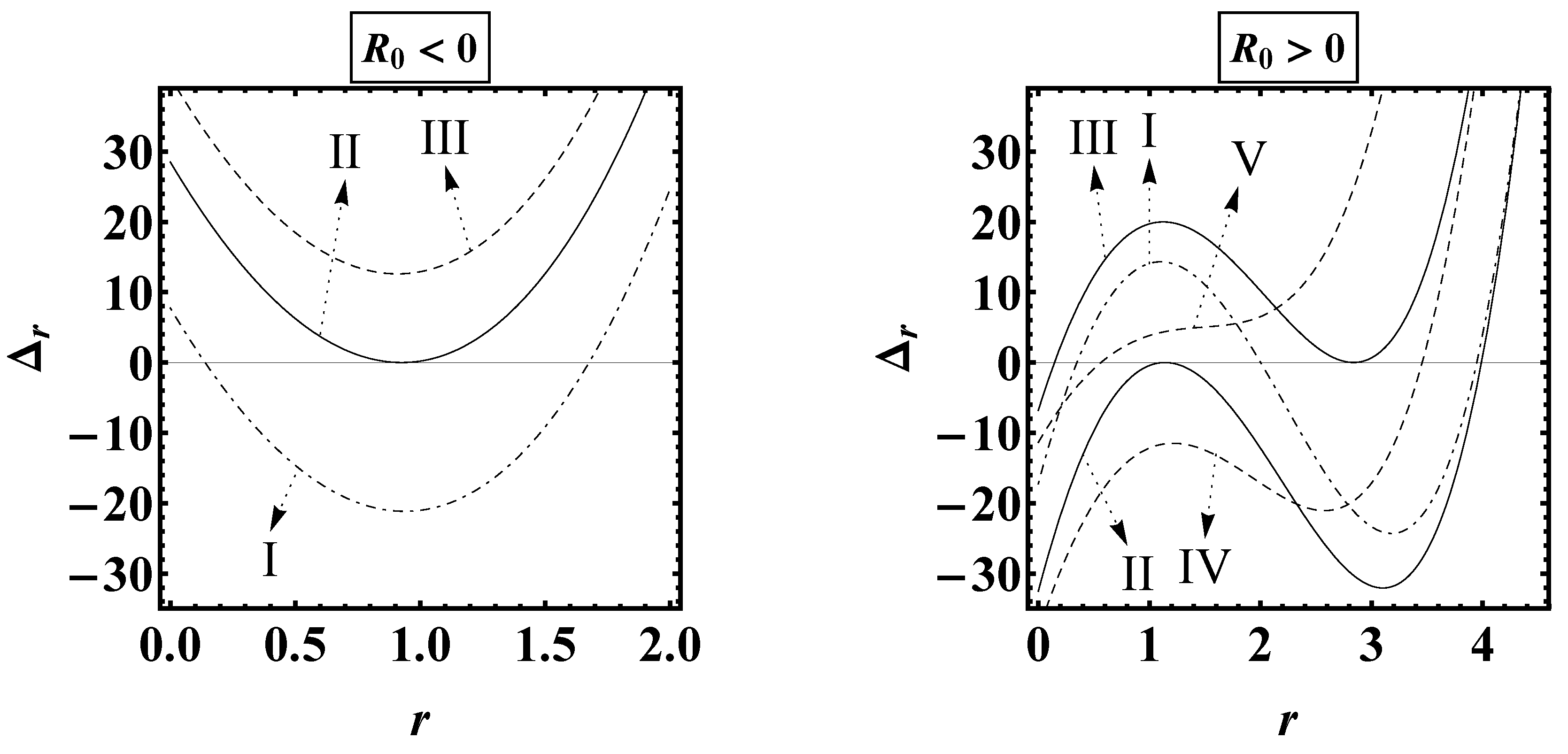
3.1. Spherically Symmetric and Static Constant Curvature Solutions: Generalities

At this stage it is interesting to ask about which are the most general static and spherically symmetric metrics with constant scalar curvature $R_0$. This curvature can be found solving the Equation (18) $R=R_0$. Thus, it is straightforward to check that, for a constant $\Phi \left(r\right)={\Phi }_0$, the general solution is [112,113]:

$$\begin{array}{c}\hfill A\left(r\right)=1+\frac{a_1}{r^{D-3}}+\frac{a_2}{r^{D-2}}-\frac{R_0}{D(D-1)}{r}^2\end{array}$$

(19)

with $a_1$ and $a_2$ being arbitrary integration constants. In fact, for the particular case $D=4$, $R_0=0$ and ${\Phi }_0=0$, the metric can be written exclusively in terms of the function:

$$\begin{array}{c}\hfill A\left(r\right)=1+\frac{a_1}{r}+\frac{a_2}{r^2}\end{array}$$

(20)

By establishing the identifications $a_1=-2G_{N}M$ and $a_2=Q^2$, this solution corresponds to a Reissner–Nordström solution, i.e., a charged massive BH solution with mass M and charge Q. Further comments about this result will be made in Section 3.2.

3.2. Spherically Symmetric and Static Constant Curvature Solutions

Let us study here which are the vacuum constant curvature solutions for $f\left(R\right)$ theories provided that the metric under consideration is of the form Equation (16)—or alternatively Equation (17). By inserting the metric Equation (16) into the general $f\left(R\right)$ gravitational action $S_g$ in Equation (8), and making variations with respect to the metric functions, $A\left(r\right)$ and $\Phi \left(r\right)$, the equations of motion become:

$$\begin{array}{c}\hfill (2-D)(1+f^{\prime }\left(R\right)){\Phi }^{\prime }\left(r\right)-r\left[f^{‴}\left(R\right)R^{\prime }{\left(r\right)}^2+f^{″}\left(R\right)({\Phi }^{\prime }\left(r\right)R^{\prime }\left(r\right)+R^{″}\left(r\right))\right]=0\end{array}$$

(21)

and

$$\begin{array}{l}2rA\left(r\right)f^{‴}\left(R\right)R^{\prime }{\left(r\right)}^2+f^{″}\left(R\right)[2DA\left(r\right)R^{\prime }\left(r\right)-4A\left(r\right)R^{\prime }\left(r\right)+2rA\left(r\right)R^{″}\left(r\right)+A^{\prime }\left(r\right)r{R}^{\prime }\left(r\right)]\\ -r(R+f\left(R\right))+g^{\prime }\left(R\right)[-2rA\left(r\right){\Phi }^{\prime }{\left(r\right)}^2+2DA\left(r\right){\Phi }^{\prime }\left(r\right)-4A\left(r\right){\Phi }^{\prime }\left(r\right)-r{A}^{″}\left(r\right)+2rA\left(r\right){\Phi }^{″}\left(r\right)\hfill \\ +A^{\prime }\left(r\right)(2-D+3r{\Phi }^{\prime }\left(r\right))]=0\hfill \end{array}$$

(22)

or alternatively in by using the metric parametrization given by Equation (17) the equations of motion now are expressed as:

$$\begin{array}{l}\lambda \left(r\right)(1+f^{\prime }\left(R\right))\left\{2\mu \left(r\right)\left[(D-2){\lambda }^{\prime }\left(r\right)+r{\lambda }^{″}\left(r\right)\right]+r{\lambda }^{\prime }\left(r\right){\mu }^{\prime }\left(r\right)\right\}\\ -2\lambda {\left(r\right)}^2\left\{2\mu \left(r\right)[(D-2)R^{\prime }\left(r\right)f^{″}\left(R\right)+r{f}^{\left(3\right)}\left(R\right)R^{\prime }{\left(r\right)}^2+r{R}^{″}\left(r\right)f^{″}\left(R\right)]+r{R}^{\prime }\left(r\right){\mu }^{\prime }\left(r\right)f^{″}\left(R\right)\right\}\hfill \\ -r\mu \left(r\right){\lambda }^{\prime }{\left(r\right)}^2(1+f^{\prime }\left(R\right))+2r\lambda {\left(r\right)}^2(R+f\left(R\right))=0\hfill \end{array}$$

(23)

and

$$\begin{array}{l}- \lambda \left(r\right){\mu }^{\prime }\left(r\right)\left[2(D-2)\lambda \left(r\right)+r{\lambda }^{\prime }\left(r\right)\right](1+f^{\prime }\left(R\right))-2r\lambda {\left(r\right)}^2(R+f\left(R\right))\\ + \mu \left(r\right)\left\{2\lambda \left(r\right)R^{\prime }\left(r\right)\left[2(D-2)\lambda \left(r\right)+r{\lambda }^{\prime }\left(r\right)\right]f^{″}\left(R\right)+r(1+f^{\prime }\left(R\right))({\lambda }^{\prime }{\left(r\right)}^2-2\lambda \left(r\right){\lambda }^{″}\left(r\right))\right\}=0\hfill \end{array}$$

(24)

where $f^{\prime }$, $f^{″}$ and $f^{‴}$ denote derivatives of $f\left(R\right)$ with respect to the curvature R. In the following calculations in this section, we use the set of Equations (21) and (22). In order to simplify the difficulty of the above equations, let us first consider here the case of constant scalar curvature $R=R_0$ solutions. Then the equations of motion Equations (21) and (22) reduce to:

$$(2-D)(1+f^{\prime }\left(R\right)){\Phi }^{\prime }\left(r\right)=0$$

(25)

and

$$\begin{array}{c}R+f\left(R\right)+(1+f^{\prime }\left(R\right))\left[A^{″}\left(r\right)+(D-2)\frac{A^{\prime }\left(r\right)}{r}-(2D-4)\frac{A\left(r\right){\Phi }^{\prime }\left(r\right)}{r}\right.\hfill \end{array}$$

$$\begin{array}{c}\left.-3A^{\prime }\left(r\right){\Phi }^{\prime }\left(r\right)+2A\left(r\right){\Phi }^{\prime 2}\left(r\right)-2A\left(r\right){\Phi }^{″}\left(r\right)\right]=0\hfill \end{array}$$

(26)

As commented in Section 2, the constant curvature solutions of $f\left(R\right)$ theories in vacuum satisfy:

$$\begin{array}{c}\hfill R_0=\frac{Df\left(R_0\right)}{2(1+f^{\prime }\left(R_0\right))-D}\end{array}$$

(27)

provided that $2(1+f^{\prime }\left(R_0\right))\ne D$. Thus from Equation (25) one concludes (excluding pathologic cases) that ${\Phi }^{\prime }\left(r\right)=0$ and then Equation (26) becomes:

$$A^{\prime \prime }\left(r\right)+(D-2)\frac{A^{\prime }\left(r\right)}{r}=-\frac{2}{D}{R}_0$$

(28)

This is a $f\left(R\right)$-independent, linear second order inhomogeneous differential equation. This statement must be understood in the sense that Equation (28) does not involve explicitly any $f\left(R\right)$ parameter. Nonetheless, it is obvious from Equation (27) that the value of $R_0$ does depend upon the $f\left(R\right)$ model under study. Therefore the metric solution $A\left(r\right)$ will also inherit information about the model under consideration. Then, Equation (28) can be easily integrated to give the general solution:

$$A\left(r\right)=C_1+\frac{C_2}{r^{D-3}}-\frac{R_0}{D(D-1)}{r}^2$$

(29)

which depends on two arbitrary constants $C_1$ and $C_2$. However, two important remarks need to be done at this stage:

• Firstly, by comparison with Equation (19), one can see that the term with the power $r^{2-D}$ is absent. This fact will be studied in Section 3.3.
• Secondly, this solution has no constant curvature in the general case since, as we found above, the constant curvature requirement demands $C_1=1$. This issue just requires a constant fixing (or equivalently a time reparametrization) and does not affect the solution.

Then, for negative $R_0$, the found solution in Equation (29) with $C_1=1$ is basically the D-dimensional generalization obtained by Witten [71] of the BH in AdS space-time solution considered by Hawking and Page [70]. With the natural choice ${\Phi }_0=0$ the solution can be written as:

$$A\left(r\right)=1-\frac{R_S^{D-3}}{r^{D-3}}+\frac{r^2}{l^2}$$

(30)

where

$$R_S^{D-3}=\frac{16\pi G_{D}M}{(D-2){\mu }_{D-2}},{\mu }_{D-2}=\frac{2{\pi }^{\frac{D-1}{2}}}{\Gamma \left(\frac{D-1}{2}\right)}$$

(31)

where ${\mu }_{D-2}$ is the area of the $D-2$ sphere, $l^2\equiv -D(D-1)/R_0$ is the asymptotic AdS space scale squared and M is the mass parameter usually found in the literature.

Thus, the main conclusion of this analysis [112,113] is that the only static and spherically symmetric vacuum solutions with constant (negative) curvature of any $f\left(R\right)$ gravity is just the Hawking–Page BH in AdS space. However this kind of solution is not the most general static and spherically symmetric metric with constant curvature, as can be seen by comparison with the solutions found in Equation (19). Therefore there exist constant curvature BH solutions that cannot be obtained as vacuum solutions of any $f\left(R\right)$ model. In particular, the term with $r^{2-D}$ power cannot be mimicked by any $f\left(R\right)$ model. As we shall show immediately, the most general solution as given by Equation (19) can be described as a charged BH solution in a $D=4f\left(R\right)$-Maxwell theory.

3.3. $f\left(R\right)$ Solutions Combined with Electromagnetism

Let us briefly mention here for completeness with the previous results the case of charged BH in $f\left(R\right)$ theories that we shall study in detail in Section 4. We shall limit ourselves to the $D=4$ case, since otherwise ($D\ne 4$) the $r^{2-D}$ term appearing in Equation (19) cannot be originated by the Maxwell action to be presented below. Let us consider here a $f\left(R\right)$ gravitational Lagrangian supplemented with the usual Maxwell action for standard Electromagnetism. Therefore, the considered action represents a generalization of the Einstein–Maxwell action:

$$S_g=\frac{1}{16\pi G_N}\int {\text{d}}^{4}x\sqrt{\mid g\mid }(R+f\left(R\right)-F_{\mu \nu }{F}^{\mu \nu })$$

(32)

where as usual $F_{\mu \nu }={\partial }_{\mu }{A}_{\nu }-{\partial }_{\nu }{A}_{\mu }$. Considering an electromagnetic potential of the form $A_{\mu }=(V\left(r\right),\overrightarrow{0})$ and the static spherically symmetric metric Equation (17), one finds that the solution with constant curvature $R_0$ reads [112,113]:

$$\begin{array}{c}\hfill V\left(r\right)=\frac{Q}{r};\lambda \left(r\right)=\mu \left(r\right)=1-\frac{2G_{N}M}{r}+\frac{1}{1+f^{\prime }\left(R_0\right)}\frac{Q^2}{r^2}-\frac{R_0}{12}{r}^2\end{array}$$

(33)

Notice that unlike the EH case, the contribution of the BH charge to the metric tensor is corrected by a ${(1+f^{\prime }\left(R_0\right))}^{-1}$ factor. This fact is of particular importance in order to constrain $f\left(R\right)$ models as astrophysically viable: the sign of the factor $1+f^{\prime }\left(R_0\right)$ needs to be positive in order to guarantee that the solution Equation (33) keeps the same sign as in the Reissner–Nordström solution. Otherwise, for a charge Q the third term in the solution Equation (33) will be negative and therefore this fact becomes experimentally observable (affecting for instance to the geodesic movements around a charged BH). In fact, the requirement $1+f^{\prime }\left(R_0\right)>0$ has been usually accepted [114] as one of the gravitational viability conditions for $f\left(R\right)$ models and is also related, as will be shown here, with thermodynamical viability.

3.4. Perturbations Around Schwarzschild–(anti)-de Sitter Solutions

In the previous section we have revised the static spherically symmetric solutions with constant curvature. In EH theory, the constant curvature ansatz Equation (27) provides the most general static and spherical symmetric solution straightforwardly. Without entering into details, this is the well-known Birkhoff–Jebsen theorem result [115,116]. However, it is not transparent for this to also be the case in $f\left(R\right)$ theories, i.e., that the most general static and spherically symmetric solution for $f\left(R\right)$ theories possesses constant curvature. Furthermore, it seems that a generic solution would behave differently in the Jordan and Einstein frames, both related by a conformal transformation, at least in the perturbative analysis (see [117,118]).

In this section we revise the basic rudiments of the perturbative analysis of the problem originally studied in [112,113], only in the Jordan frame. In that analysis, it was assumed that the modified gravitational Lagrangian is a small perturbation around the EH Lagrangian. Therefore, the arbitrary $f\left(R\right)$ function is of the form:

$$\begin{array}{c}\hfill f\left(R\right)=-(D-2){\Lambda }_D+\alpha g\left(R\right)\end{array}$$

(34)

where $\alpha \ll 1$ is a dimensionless parameter and $g\left(R\right)$ is assumed to be analytic in α. This last assumption is based on the fact that the scalar curvature R is also α-dependent as will be seen in expressions Equation (35). Therefore $g\left(R\right)$ may also be expanded in powers of α. By assumption and for the sake of simplicity, $g\left(R\right)$ is assumed analytic in the expansion in powers of α.

Now, assuming that the $\lambda \left(r\right)$ and $\mu \left(r\right)$ functions appearing in the metric Equation (17) are also analytical in α, they can be written as follows:

$$\begin{array}{c}\hfill \lambda \left(r\right)={\lambda }_0\left(r\right)+\sum _{i=1}^{\infty }{\alpha }^i{\lambda }_i\left(r\right),\mu \left(r\right)={\mu }_0\left(r\right)+\sum _{i=1}^{\infty }{\alpha }^i{\mu }_i\left(r\right)\end{array}$$

(35)

where $\{{\lambda }_0\left(r\right),{\mu }_0\left(r\right)\}$ are the unperturbed solutions for the EH action with cosmological constant, i.e., S(A)dS solution, given by:

$$\begin{array}{c}\hfill {\mu }_0\left(r\right)=1+\frac{C_1}{r^{D-3}}-\frac{{\Lambda }_D}{(D-1)}{r}^2,{\lambda }_0\left(r\right)=-C_2(D-2)(D-1){\mu }_0\left(r\right)\end{array}$$

(36)

which are the standard BH solutions in a D-dimensional Schwarzschild–(A)dS space-time. The factor $C_2$ can be chosen by performing a coordinate t reparametrization so that both functions in Equation (36) can be identified. For the moment, the background solutions are kept as given in Equation (36) since the possibility of getting $\lambda \left(r\right)=\mu \left(r\right)$ in the perturbative expansion will be discussed later on.

The perturbative procedure is as follows: by inserting Equations (34) and (35) into the general Einstein modified Equations (23) and (24), equations for each order in α parameter powers are obtained. Please refer to [112,113] for details.

Notice that from the obtained results up to second order in α, the corresponding metric has constant scalar curvature for any value of the integration constants. As a matter of fact, this metric is nothing but the standard Schwarzschild–(A)dS geometry, and can be easily recast in the usual form by making a trivial reparametrization in the time coordinate.

Therefore, this analysis proved that at least up to second order, the only static, spherically symmetric solutions which are analytical in α are the standard Schwarzschild–AdS space-times irrespectively of the $f\left(R\right)$ model under consideration. This result is valid provided that both the solutions and the gravitational Lagrangian are analytic in the α parameter and that $g\left(R\right)$ corresponds to a small deviation from the usual EH gravitational Lagrangian. Further orders in ${\alpha }^{3,4,...}$ can be obtained by inserting previous results in the equations of order $3,4,...$ and so on. This way one may get the solutions $\{{\lambda }_{3,4,...}\left(r\right),{\mu }_{3,4,...}\left(r\right)\}$ with the added difficulty that the corresponding equations become more and more complicated.

To conclude Section 3 and Section 3.4, we can summarize by saying that in the context of $f\left(R\right)$ gravities the only spherically symmetric and static solutions of negative constant curvature are the standard BH in AdS space. The same result applies in the general case (without imposing constant curvature) in perturbation theory up to second order. However, the possibility of having static and spherically symmetric solutions with non-constant curvature cannot be excluded in the case of $f\left(R\right)$ functions, which are not analytical in α parameter.

4. Kerr–Newman Black Holes in $f\left(R\right)$ Theories

In this section, we shall focus our attention in obtaining constant curvature $R_0$ vacuum solutions for fields generated by massive charged objects in the frame of $f\left(R\right)$ gravity theories. Hence, the appropriate action to derive the field equations will be now Equation (32) and $D=4$ will be assumed throughout this section. The obtained equations (in $G_N=c=\hslash =k_B=1$ units) are:

$$\begin{array}{c}\hfill R_{\mu \nu }(1+f^{\prime }\left(R_0\right))-\frac{1}{2}{g}_{\mu \nu }(R_0+f\left(R_0\right))-2\left(F_{\mu \alpha }{F}_{\nu }^{\alpha }-\frac{1}{4}{g}_{\mu \nu }{F}_{\alpha \beta }{F}^{\alpha \beta }\right)=0\end{array}$$

(37)

In the studied case $D=4$, the trace of the previous equation leads again to expression Equation (27) due to the conformal character of the Faraday tensor, i.e., $F^{\mu }{}_{\mu }=0$.

For these $f\left(R\right)$ field equations the axisymmetric, stationary and constant curvature $R_0$ solution that describes a BH with mass, electric charge and angular momentum is analogous to the one found by Carter and published for the first time in 1973 [119]. In Boyer–Lindquist coordinates, the metric takes the form [120,121]:

$$\begin{array}{c}\hfill \text{d}{s}^2=\frac{{\rho }^2}{{\Delta }_r}\text{d}{r}^2+\frac{{\rho }^2}{{\Delta }_{\theta }}\text{d}{\theta }^2+\frac{{\Delta }_{\theta }{sin}^2\theta }{{\rho }^2}{\left[a\frac{\text{d}t}{\Xi }-\left(r^2+a^2\right)\frac{\text{d}\varphi }{\Xi }\right]}^2-\frac{{\Delta }_r}{{\rho }^2}{\left(\frac{\text{d}t}{\Xi }-a{sin}^2\theta \frac{\text{d}\varphi }{\Xi }\right)}^2\end{array}$$

(38)

with

$$\begin{array}{ccc}\hfill {\Delta }_r& :=& \left(r^2+a^2\right)\left(1-\frac{R_0}{12}{r}^2\right)-2Mr+\frac{Q^2}{\left(1+f^{\prime }\left(R_0\right)\right)}\hfill \end{array}$$

$$\begin{array}{c}\hfill {\rho }^2:=r^2+a^2{cos}^2\theta ;{\Delta }_{\theta }:=1+\frac{R_0}{12}{a}^2{cos}^2\theta ;\Xi :=1+\frac{R_0}{12}{a}^2\end{array}$$

(39)

where M, a and Q denote the mass, spin and electric charge parameters respectively. Notice that, unlike in the GR case, the contribution of the charge of the BH to the metric is corrected by a ${\left(1+f^{\prime }\left(R_0\right)\right)}^{-1/2}$ factor. This feature was already obtained for Reissner–Nordström BH presented in expression Equation (33) and originally in [112,113]. On the other hand, the required potential vector and electromagnetic field tensor in Equation (37) solutions for metric Equation (38) are respectively:

$$\begin{array}{ccc}\hfill A& =& -\frac{Qr}{{\rho }^2}\left(\frac{\text{d}t}{\Xi }-a{sin}^2\theta \frac{\text{d}\varphi }{\Xi }\right),\hfill \\ \hfill F& =& -\frac{Q(r^2-a^2{cos}^2\theta )}{{\rho }^4}\left(\frac{\text{d}t}{\Xi }-a{sin}^2\theta \frac{\text{d}\varphi }{\Xi }\right)\wedge \text{d}r-\frac{2Qracos\theta sin\theta }{{\rho }^4}\text{d}\theta \wedge \left[a\frac{\text{d}t}{\Xi }-(r^2+a^2)\frac{\text{d}\varphi }{\Xi }\right]\hfill \end{array}$$

(40)

To lighten notation, from now on let us use the notation ${\overline{Q}}^2\equiv Q^2/\left(1+f^{\prime }\left(R_0\right)\right)$ as a normalized electric charge parameter of the BH.

4.1. Event Horizons

Let us now briefly study the horizon structure of these BH: according to the event horizon definition, i.e., $g^{rr}=0$, these hypersurfaces are found as the roots of the equation ${\Delta }_r=0$, i.e.,

$$\begin{array}{c}\hfill r^4+\left(a^2-\frac{12}{R_0}\right)r^2+\frac{24M}{R_0}r-\frac{12}{R_0}\left(a^2+{\overline{Q}}^2\right)=0\end{array}$$

(41)

This is an algebraic fourth order equation that, following [120,121], can be rewritten as:

$$\begin{array}{c}\hfill (r-r_{-})(r-r_{int})(r-r_{ext})(r-r_{cosm})=0\end{array}$$

(42)

where

• $r_{-}$ is always a negative solution with no physical meaning,
• $r_{int}$ and $r_{ext}$ are the interior and exterior horizon respectively, and
• $r_{cosm}$ represents—provided that it arises—the cosmological event horizon for observers between $r_{ext}$ and $r_{cosm}$.

The latter divides the accessible region from the hidden region for an exterior observer. The Equation (42) can be solved by using L. Ferrari’s method for quartic equations. The existence of real solutions for this equation is given by a factor h, which we shall denote as horizon parameter:

$$\begin{array}{ccc}\hfill h\equiv & & {\left[\frac{4}{R_0}{\left(1-\frac{R_0}{12}{a}^2\right)}^2-4\left(a^2+{\overline{Q}}^2\right)\right]}^3\hfill \\ & & +\frac{4}{R_0}{\left\{\left(1-\frac{R_0}{12}{a}^2\right)\left[\frac{4}{R_0}{\left(1-\frac{R_0}{12}{a}^2\right)}^2+12\left(a^2+{\overline{Q}}^2\right)\right]-18M^2\right\}}^2.\hfill \end{array}$$

(43)

In Figure 1 we show the zeros of the fourth order polynomial ${\Delta }_r$ that lead to different astrophysical configurations, depending on the values and signs of $R_0$ and h.

Figure 1. Graphics showing horizons positions as solutions of the equation ${\Delta }_r=0$ taken from [120,121]. On the left panel ($R_0<0$) the presented cases are: $h>0$ (I), BH with well-defined horizons, dashed with dots), $h=0$ (II), extremal BH, continuous line) and $h<0$ (III), naked singularity, dashed). On the right panel ($R_0>0$) the represented cases are: $h<0$ (I, BH with well-defined horizons, dashed with dots), $h=0$ (II, $extremal$ BH and III, $extremal$ $marginal$ BH, continuous line), and $h>0$ (IV, naked singularity and V, naked marginal singularity, dashed).

Figure 1. Graphics showing horizons positions as solutions of the equation ${\Delta }_r=0$ taken from [120,121]. On the left panel ($R_0<0$) the presented cases are: $h>0$ (I), BH with well-defined horizons, dashed with dots), $h=0$ (II), extremal BH, continuous line) and $h<0$ (III), naked singularity, dashed). On the right panel ($R_0>0$) the represented cases are: $h<0$ (I, BH with well-defined horizons, dashed with dots), $h=0$ (II, $extremal$ BH and III, $extremal$ $marginal$ BH, continuous line), and $h>0$ (IV, naked singularity and V, naked marginal singularity, dashed).

Let us stress at this stage that, from a certain positive value of the curvature $R_0^{crit}$ onward, the h factor goes to zero for two values of a. They can be understood as follows:

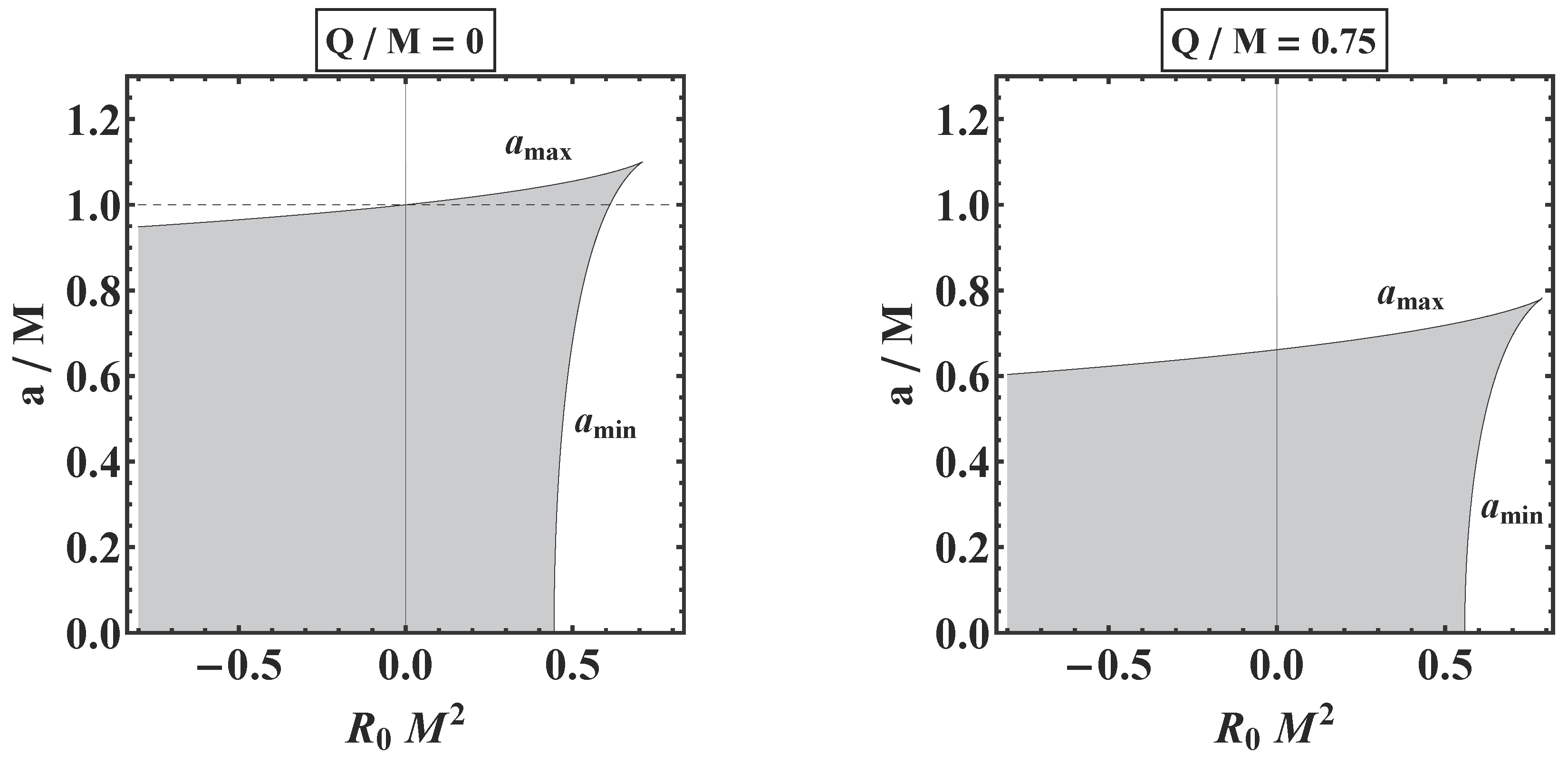
• Upper spin bound, $a=a_{max}$ for which the BH turns $extremal$—the interior and exterior horizons have merged into a single horizon with a null surface gravity. This is the usual configuration for the BH to become extremal.
• Lower spin bound, $a=a_{min}$, below which the BH turns into a marginal extremal BH. This value can be understood as the cosmological limit for which a BH preserves its exterior horizon without being “torn apart" due to the relative recession speed between two radially separated points induced by the cosmic expansion [120,121].

In Figure 2 we revisit the original plot shown in [120,121], where for certain values of the electric charge parameter $\overline{Q}$ the allowed ranges of the spin a parameter values are presented.

Figure 2. The shaded regions, delimited by the upper $a_{max}$ and lower $a_{min}$ curves, represent the values of $a/M$ for which the existence of BH is possible once $R_0{M}^2$ value is fixed. Panels show for $\overline{Q}/M=0$ (left) and $\overline{Q}/M=0.75$ (right) on the left and right panels respectively. Note that $R_0$ has dimensions of [length]${}^{-2}$ when normalizing. Original plots at [120,121].

Figure 2. The shaded regions, delimited by the upper $a_{max}$ and lower $a_{min}$ curves, represent the values of $a/M$ for which the existence of BH is possible once $R_0{M}^2$ value is fixed. Panels show for $\overline{Q}/M=0$ (left) and $\overline{Q}/M=0.75$ (right) on the left and right panels respectively. Note that $R_0$ has dimensions of [length]${}^{-2}$ when normalizing. Original plots at [120,121].

5. Black Holes Thermodynamics in $f\left(R\right)$ Theories

As mentioned in the Introduction, the study of BH thermodynamics has drawn a lot of attention when studying these configurations in alternative theories of gravity. We shall divide this section in two main parts: the study of thermodynamics in AdS case and then the study of KN case as the natural generalization of the former. This approach will enable to introduce first the rudiments of the Euclidean method so the reader can familiarize with it, and then extend the formulation for more general objects such as the KN BH configurations. Finally, we will provide some examples by considering $f\left(R\right)$ models that illustrate the procedure for both configurations. In the AdS case, the dimension of the space-time will be arbitrary and then fixed to several values in order to illustrate the found results. On the contrary, for the KN study, dimension will be fixed from the very beginning to $D=4$ for the sake of simplicity.

5.1. BH Thermodynamics for AdS Configuration

In order to study the different thermodynamic quantities for the $f\left(R\right)$ BH in AdS space, the temperature is usually considered as the basic quantity from which the rest of the thermodynamic quantities are derived. In principle, there are two different approaches of introducing this quantity for the AdS solutions. Firstly, one of the possible definitions is the one provided by the Euclidean quantum gravity [122,123,124,125] that was revised in [112,113] yielding:

$$T_E=\frac{1}{4\pi }{e}^{-\Phi \left(r_H\right)}{A}^{\prime }\left(r_H\right)$$

(44)

Another possible definition of temperature was firstly proposed in [126] stating that temperature can be given in terms of the horizon gravity $\mathcal{K}$ as $T_{\mathcal{K}}\equiv \frac{\mathcal{K}}{4\pi }$. Then, by reminding the metric definition Equation (16), it is straightforward to obtain that $T_{\mathcal{K}}=T_E$. In conclusion, both definitions lead to the same result for this kind of solution. Notice also that in any case the temperature depends only on the behavior of the metric near the horizon and it is independent of the underlying gravitational action. This last statement can be understood by remarking that either different actions or different field equations giving rise to the same solutions of the form Equation (16) will also present the same temperature. This is not the case for other thermodynamic quantities as will be seen later. Taking into account the results in previous sections, the usual analyses for $f\left(R\right)$ theories [112,113] have focused on the constant curvature AdS BH solutions with $\Phi =0$ as a natural choice, and $A\left(r\right)$ as given by expression Equation (30). Then, both definitions of temperature lead to:

$$\beta \equiv \frac{1}{T}=\frac{4\pi l^2{r}_H}{(D-1)r_H^2+(D-3)l^2}$$

(45)

Notice that for a given dimension D, the temperature is a function of $r_H$ only, i.e., it depends only on the BH size. In the limit $r_H$ going to zero the temperature diverges as $T\sim 1/r_H$ and for $r_H$ going to infinite T grows linearly with $r_H$. Consequently T has a minimum corresponding to a temperature:

$$T_0=\frac{\sqrt{(D-1)(D-3)}}{2\pi l}$$

(46)

The existence of this minimum was established in [70] for $D=4$ by Hawking and Page. More recently, Witten extended this result to higher dimensions [71]. This minimum will be relevant in order to set the regions with different thermodynamic behaviors and stability properties.

Explicit solutions for $A\left(r_H\right)=0$ in Equation (30) can be found for $D=4,5$ and were found in [112,113].

Another important temperature value is the one corresponding to a horizon radius $r_H=l$. Let us denote it as $T_1$ and from Equation (45) it is given by:

$$T_1=\frac{D-2}{2\pi l}$$

(47)

Notice that for $D>2$ we have $T_0<T_1$.

In order to compute the remaining thermodynamic quantities, the standard procedure is to consider the D-dimensional Euclidean action defined as follows:

$$S_E=-\frac{1}{16\pi G_D}\int {\text{d}}^{D}x\sqrt{g_E}(R+f\left(R\right))$$

(48)

When the previous expression is evaluated on some metric with a periodic Euclidean time of period β, it equals β times the free energy F associated to this metric. The computation by Hawking and Page [70], generalized to higher dimensions by Witten [71], was extended to $f\left(R\right)$ theories in [72] and [112,113]. In these references the difference of this action, when it is evaluated on the BH and on the AdS metric, was computed leading to:

$$\Delta S_E=-\frac{(R_0+f\left(R_0\right))\beta {\mu }_{D-2}}{32\pi (D-1)G_D}(l^2{r}_H^{D-3}-r_H^{D-1})=\beta F$$

(49)

where $R_0=-D(D-1)/l^2$. From this expression it is straightforward to obtain the free energy as $F=\Delta S_E/\beta$. One can also see that provided that the condition $-(R_0+f\left(R_0\right))>0$ is fulfilled—which is the usual case in EH gravity—we have $F>0$ for $r_H<l$ and $F<0$ for $r_H>l$.

Once that both temperature and free energy have been calculated, the total thermodynamical energy may now be obtained as:

$$E\equiv \frac{\partial \Delta S_E}{\partial \beta }=-\frac{(R_0+f\left(R_0\right))M{l}^2}{2(D-1)}$$

(50)

where M is the mass defined in Equation (31). This is one of the possible definitions for the BH energy for $f\left(R\right)$ theories but other definitions are available in the literature, see for instance [127] for a more general discussion. For the EH action with non-vanishing cosmological constant, we have $f\left(R\right)=-(D-2){\Lambda }_D$ and then it is immediate to find $E=M$. However this is not the case for general $f\left(R\right)$ gravitational Lagrangians as seen in Equation (50). Notice that positive energy in AdS space-time requires $R_0+f\left(R_0\right)<0$.

Now the entropy S can be obtained from the well-known relation $S\equiv \beta E-\beta F$. Then one gets:

$$S=-\frac{(R_0+f\left(R_0\right))l^2{A}_{D-2}\left(r_H\right)}{8(D-1)G_D}$$

(51)

where $A_{D-2}\left(r_H\right)$ is the horizon area given by $A_{D-2}\left(r_H\right)\equiv r_H^{D-2}{\mu }_{D-2}$. Notice that once again positive entropy requires $R_0+f\left(R_0\right)<0$. For the EH action non-vanishing cosmological constant, we have $R_0+f\left(R_0\right)=-2(D-1)/l^2$ and then the famous Hawking–Bekenstein result [128] is recovered:

$$S=\frac{A_{D-2}\left(r_H\right)}{4G_D}$$

(52)

Finally we can compute the heat capacity C which can be written as:

$$C\equiv \frac{\partial E}{\partial T}=\frac{\partial E}{\partial r_H}\frac{\partial r_H}{\partial T}$$

(53)

Then it is easy to find:

$$C=\frac{-(R_0+f\left(R_0\right))(D-2){\mu }_{D-2}{r}_H^{D-2}{l}^2}{8G_D(D-1)}\frac{(D-1)r_H^2+(D-3)l^2}{(D-1)r_H^2-(D-3)l^2}$$

(54)

For the particular case of the EH action with cosmological constant we find:

$$C=\frac{(D-2){\mu }_{D-2}{r}_H^{D-2}}{4G_D}\frac{(D-1)r_H^2+(D-3)l^2}{(D-1)r_H^2-(D-3)l^2}$$

(55)

In the Schwarzschild limit, i.e., l going to infinity, this formula turns into:

$$C=-\frac{(D-2){\mu }_{D-2}{r}_H^{D-2}}{4G_D}<0$$

(56)

which is the well-known result for standard Schwarzschild BH, i.e., $C<0$.

Provided that the condition $(R_0+f\left(R_0\right))<0$ is accomplished, the $f\left(R\right)$ general case lead, like in the EH case, to $C>0$ for $r_H>r_{H0}$ (the large BH region) and $C<0$ for $r_H<r_{H0}$ (the small BH region). For $r_H\sim r_{H0}$ (T close to $T_0$) C is divergent. Notice that in EH gravity, $C<0$ necessarily implies $F>0$ since $T_0<T_1$.

In summary, $f\left(R\right)$ theories accomplishing the condition:

$$\begin{array}{c}\hfill R_0+f\left(R_0\right)<0\end{array}$$

(57)

provide a scenario analogous to the one described in full detail by Hawking and Page in [70] for the EH case. This analysis was originally shown in [112,113] and then widely used in literature.

In principle, particular $f\left(R\right)$ models violating the condition $R_0+f\left(R_0\right)<0$ can be naively considered. However, in such cases, the mass and the entropy would be negative and therefore the AdS BH solutions for these models would be unphysical. Therefore $R_0+f\left(R_0\right)<0$ can be regarded as a necessary condition for $f\left(R\right)$ theories in order to support the usual AdS BH solutions. Using Equation (27), this condition is fully equivalent to $1+f^{\prime }\left(R_0\right)>0$. This last condition has a clear physical interpretation in $f\left(R\right)$ gravity theories (see [114] and references therein). Indeed, it can be interpreted as the condition for the effective Newton constant $G_{eff}=G_D/(1+f^{\prime }\left(R_0\right))$ to be positive. It can also be interpreted from the quantum point of view as the condition which prevents the graviton from becoming a ghost. Therefore the requirement Equation (57) can be also regarded as a thermodynamical viability condition for $f\left(R\right)$ gravity theories when AdS configurations are studied [112,113].

Once that the main thermodynamical quantities have been derived, let us now revise the local and global stabilities phenomenology: For $T<T_0$, the only possible state of thermal equilibrium in an AdS space is pure radiation with negative free energy and hence there is no stable BH solutions. For $T>T_0$ there exist two possible BH solutions; the small (and light) BH and the large (heavy) BH. The small one has negative heat capacity and positive free energy as the standard Schwarzschild BH. Therefore it is unstable under Hawking radiation decay. For the large BH there appear two possibilities; if $T_0<T<T_1$ then both the heat capacity and the free energy are positive and the BH will decay by tunneling into radiation, but if $T>T_1$ then the heat capacity is still positive but the free energy becomes negative. In this case the free energy of the heavy BH will be less than that of pure radiation. Then pure radiation will tend to tunnel or to collapse to the BH configuration in equilibrium with thermal radiation. This phenomenology will be applied to different $f\left(R\right)$ models in Section 6.

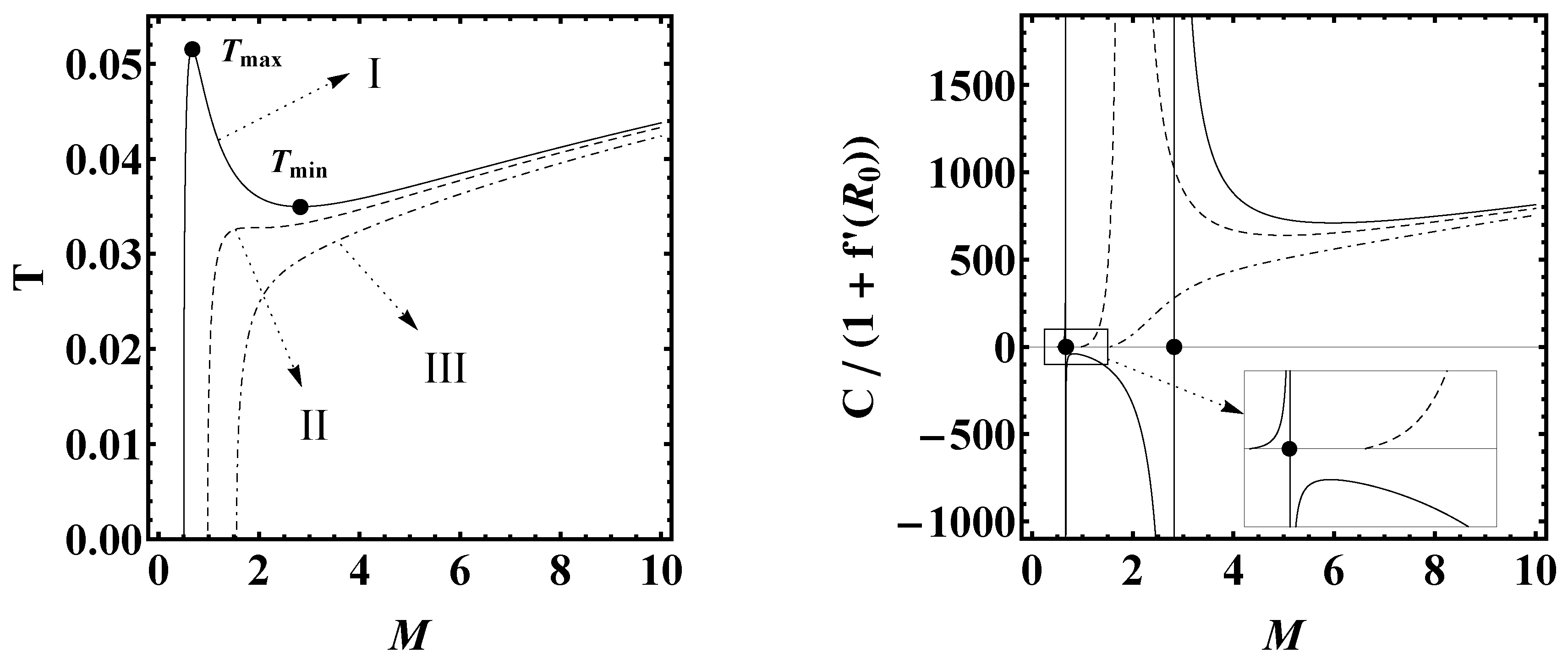
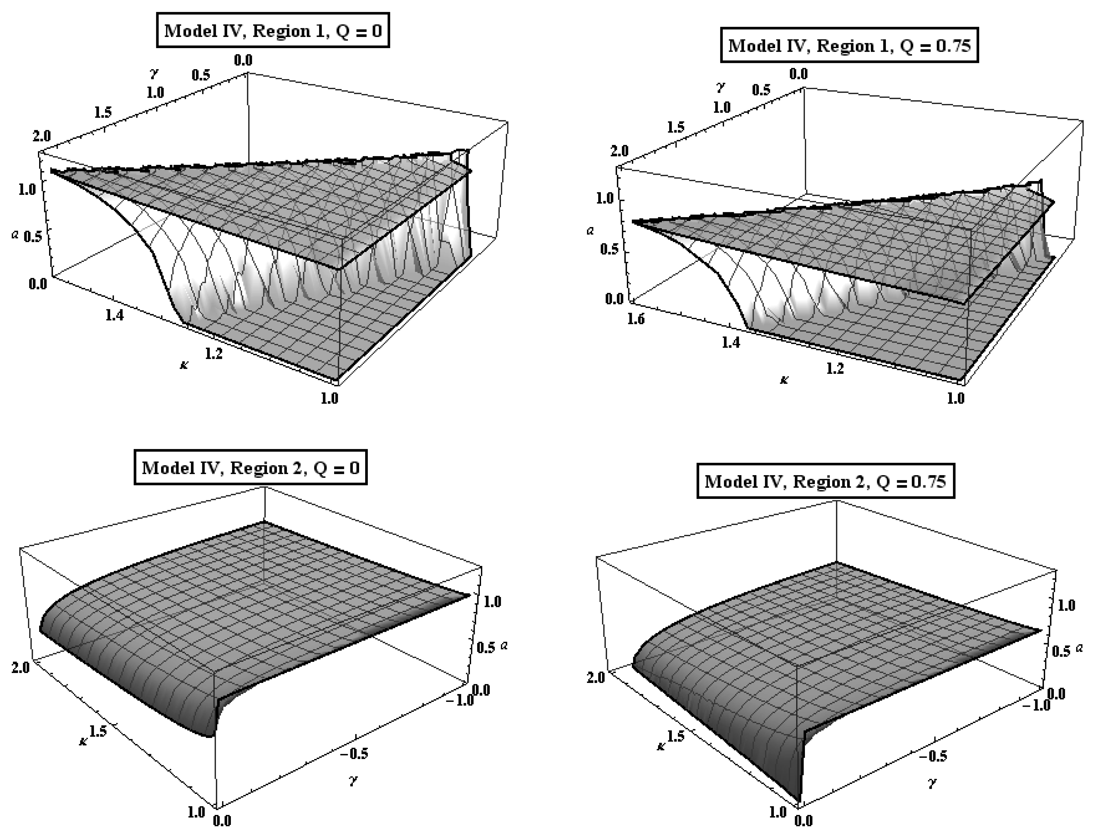
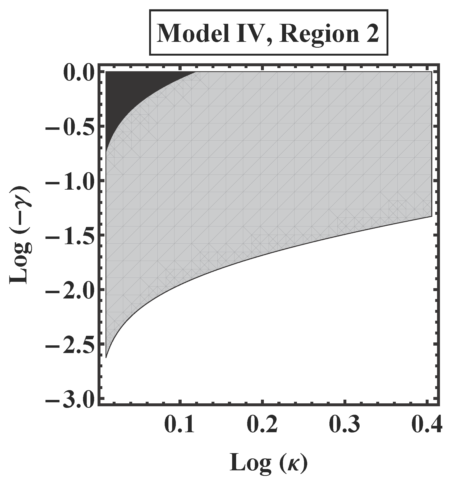
5.2. BH Thermodynamics for KN Configuration

Following the reasoning at the beginning of this section, the research concerning the KN configuration will be also done for BH with a well-defined horizon structure for negative values of $R_0$. In order to study the different thermodynamical properties of Kerr–Newman BH in $f\left(R\right)$ theories, the usual approach is to start studying the temperature of the exterior horizon $r_{ext}\equiv r_{ext}\left(R_0,a,\overline{Q},M\right)$. For that purpose, the Euclidean action method [122,123,124,125] is again considered. The procedure consists now of performing the change of variables $t\to -i\tau$, $a\to ia$ on the metric (38) in order to obtain the Euclidean section (see [120,121] for details). After some calculations, the inverse Hawking temperature now becomes:

$$\begin{array}{c}\hfill {\beta }_{\text{KN}}\equiv \frac{1}{T_{E,\text{KN}}}=\frac{{\displaystyle 4\pi \left(r_{ext}^2+a^2\right)}}{{\displaystyle r_{ext}\left[1-\frac{R_0{a}^2}{12}-\frac{R_0{r}_{ext}^2}{4}-\frac{\left(a^2+{\overline{Q}}^2\right)}{r_{ext}^2}\right]}}\end{array}$$

(58)

For null spin and charge, this expression becomes naturally Equation (45).

BH horizon temperature can also be obtained through Killing vectors, as is explained in [126] where temperature is defined as: $T_{\kappa ,\text{KN}}\equiv \kappa /4\pi$, with κ the surface gravity defined now as ${\chi }^{\mu }{\nabla }_{\mu }{\chi }_{\nu }=\kappa {\chi }_{\nu }$. It can be verified that κ is the same at any horizon point and consequently $T_{\kappa ,\text{KN}}=T_{E,\text{KN}}$ as obtained in [129].

Now that we know the expression for the temperature for KN configurations, the natural step in order to obtain the remaining thermodynamical quantities is to consider the corresponding extension of the Euclidean action with respect to the previously considered Equation (48). It now becomes:

$$\begin{array}{c}\hfill \Delta S_{E,\text{KN}}=\frac{1}{16\pi }{\int }_{\mathcal{Y}}{\text{d}}^{4}x\sqrt{\mid g\mid }\left(R_0+f\left(R_0\right)-F_{\mu \nu }{F}^{\mu \nu }\right)\end{array}$$

(59)

with $\mathcal{Y}$ the integration region. As is described in [70], and fully derived in [120,121] the result for $\Delta S_{E,\text{KN}}$ becomes:

$$\begin{array}{c}\hfill \Delta S_{E\text{KN}}=\frac{\beta \left(R_0+f\left(R_0\right)\right)}{24\Xi }\left[r_{ext}^3+\left(a^2+\frac{12}{R_0}\right)r_{ext}+\frac{12a^2}{R_0{r}_{ext}}\right]+\frac{\beta }{2}{\Phi }_e\mathcal{Q}\left(\frac{r_{ext}^2+a^2}{2r_{ext}^2}+1\right)\end{array}$$

(60)

where ${\Phi }_e$ is the electric potential of the horizon as seen from infinity:

$$\begin{array}{c}\hfill {\Phi }_e\equiv \frac{Q{r}_{ext}}{r_{ext}^2+a^2}=\frac{\overline{Q}{r}_{ext}}{r_{ext}^2+a^2}{\left(1+f^{\prime }\left(R_0\right)\right)}^{1/2}\end{array}$$

(61)

and $\mathcal{Q}$ is the physical electric charge of the BH, obtained by integrating the flux of the electromagnetic field tensor at infinity, which happens to be:

$$\begin{array}{c}\hfill \mathcal{Q}\equiv \frac{Q}{\Xi }=\frac{\overline{Q}}{\Xi }{\left(1+f^{\prime }\left(R_0\right)\right)}^{1/2}\end{array}$$

(62)

From expressions Equations (61) and (62), it can be seen that ${\Phi }_e$ and $\mathcal{Q}$ definitions are $f\left(R\right)$-model independent. The reason for this lies in the fact that these calculations involve the vector potential and the electromagnetic field tensor, which are independent of the considered $f\left(R\right)$ model. Further analysis of the action revealed [120,121] that it became singular for $h=0$, as could be expected from extremal BH, whose temperature $T_{E,\text{KN}}=0$ makes the ${\beta }_{\text{KN}}$ factor diverge. Since thermodynamical potentials are obtained by dividing the action by the β factor, they still remain well-defined at $T_{E,\text{KN}}=0$.

By using the expression Equation (60) we can immediately obtain Helmholtz free energy F. For rotating configurations, the correct definition is now:

$$\begin{array}{c}\hfill F=\frac{\Delta S_E}{\beta }+{\Omega }_{H}J\end{array}$$

(63)

where the term ${\Omega }_{H}J$ comes from the required Legendre transformation to fix angular momentum, being J the angular momentum of the BH and ${\Omega }_H$ the angular velocity of the rotating horizon. For the explicit expressions, we refer the reader to [120,121]. Thus, performing some calculations one gets:

$$\begin{array}{c}\hfill F=(1+f^{\prime }\left(R_0\right))\frac{{\displaystyle \left[36{\overline{Q}}^2+12r_{ext}^2+r_{ext}^4{R}_0+a^2(36-r_{ext}^2{R}_0)\right]}}{{\displaystyle 24r_{ext}\Xi }}\end{array}$$

(64)

Once again, expression Equation (64) reduces to Equation (49) for a non-rotating uncharged BH. Provided that the condition $1+f^{\prime }\left(R_0\right)>0$ is required to hold in order to obtain positive values of the mass, the inspection of the numerator of F renders that $F>0$ for values of the horizon below $r_{ext}^{\mathit{\text{limit}}}$ (with an associated mass $M^{\mathit{\text{limit}}}$ through Equation (41)), and $F<0$ for larger values.

Using the appropriate thermodynamical relations [130], we can derive the entropy S of the KN BH, which reads:

$$\begin{array}{c}\hfill S=\beta (\mathcal{M}-{\Omega }_{H}J)-\Delta S_E=(1+f^{\prime }\left(R_0\right))\frac{\pi (r_{ext}^2+a^2)}{{\displaystyle \Xi }}\end{array}$$

(65)

If the area ${\mathcal{A}}_H$ of the exterior horizon is now computed, one gets:

$$\begin{array}{c}\hfill {\mathcal{A}}_H=4\pi (r_{ext}^2+a^2)/\Xi \end{array}$$

(66)

Thus, if expression Equation (66) is substituted into the entropy expression Equation (65), the entropy can be expressed as:

$$\begin{array}{c}\hfill S=(1+f^{\prime }\left(R_0\right))\frac{{\mathcal{A}}_H}{4}\end{array}$$

(67)

Consequently $1+f^{\prime }\left(R_0\right)>0$ is again a mandatory condition to obtain a positive entropy, as was shown in the AdS as well. Note that if for example we want to recover GR with a cosmological constant taking $f\left(R_0\right)=-2\Lambda$, this relation turns into: $S={\mathcal{A}}_H/4$, i.e., the famous Bekenstein result [128].

Once that the temperature T and the entropy S of the KN BH are known, the natural step further can be taken and study the heat capacity at constant scalar curvature $R_0$ and at fixed spin a and charge $\overline{Q}$ parameters. From the definition:

$$\begin{array}{c}\hfill C=T{\left.\frac{\partial S}{\partial T}\right|}_{R_0,a,Q}\end{array}$$

(68)

we obtain the expression:

$$\begin{array}{c}\hfill C=(1+f^{\prime }\left(R_0\right))\frac{{\displaystyle 2\pi r_{ext}^2(a^2+r_{ext}^2)\left[a^2(12+r_{ext}^2{R}_0)+3(4{\overline{Q}}^2-4r_{ext}^2+r_{ext}^4{R}_0)\right]}}{Den(\overline{Q},r_{ext},R_0,a)}\end{array}$$

(69)

with $Den(\overline{Q},r_{ext},R_0,a)\equiv Den$ defined as:

$$\begin{array}{c}\hfill Den\equiv \Xi \left[-36{\overline{Q}}^2{r}_{ext}^2+a^4(-12+r_{ext}^2{R}_0)+3r_{ext}^4(4+r_{ext}^2{R}_0)-4a^2(3{\overline{Q}}^2+12r_{ext}^2-2r_{ext}^4{R}_0)\right]\end{array}$$

At this stage, it is interesting to find out for which values of $R_0$, a, $\overline{Q}$ and M the denominator of the thermal capacity becomes zero, i.e., the thermal capacity goes through an infinite discontinuity, i.e., the BH experiences a phase transition. Following the analysis presented in [120,121], two kinds of BH on this subject can be distinguished depending on the values of the a, $\overline{Q}$ and M parameters and scalar curvature $R_0$:

• fast BH, without phase transitions and always positive heat capacity $C>0$.
• slow BH, presents two phase transitions for two determined values of $r_{ext}$.

In Figure 3 we have visualized the behavior of the temperature T and the heat capacity C of a BH for different values of mass parameter M, with fixed a, $\overline{Q}$ and $R_0$ values.

Figure 3. For $R_0=-0.2$, we graphically display temperature (left) and heat capacity (right) of a BH as functions of the mass parameter M for the cases: (I) $a=0.5$ y $Q=0$ : “slow” BH that shows a local maximum temperature $T_{max}$ and a local minimum temperature $T_{min}$ at the points where the heat capacity diverges, taking the latter negative values between $T_{max}$ y $T_{min}$; (II) $a\approx 0.965$ y $Q=0$ : limit case where $T_{max}$ and $T_{min}$ merge, hence resulting in an inflection point in the temperature and an always positive heat capacity; (III) $a=1.5$ y $Q=0$ : “fast” BH with both temperature and heat capacity monotonously growing (always positive too).

Figure 3. For $R_0=-0.2$, we graphically display temperature (left) and heat capacity (right) of a BH as functions of the mass parameter M for the cases: (I) $a=0.5$ y $Q=0$ : “slow” BH that shows a local maximum temperature $T_{max}$ and a local minimum temperature $T_{min}$ at the points where the heat capacity diverges, taking the latter negative values between $T_{max}$ y $T_{min}$; (II) $a\approx 0.965$ y $Q=0$ : limit case where $T_{max}$ and $T_{min}$ merge, hence resulting in an inflection point in the temperature and an always positive heat capacity; (III) $a=1.5$ y $Q=0$ : “fast” BH with both temperature and heat capacity monotonously growing (always positive too).

As was remarked in [120,121], KN–AdS BH, unlike Schwarzschild–AdS BH case [70], are allowed for any value of the temperature T. Hence stability of each BH will be exclusively given by the corresponding values of heat capacity C and free energy F as functions of the a, $\overline{Q}$, M and $R_0$ parameters, that ultimately define the BH. However, for a set of fixed values of a, $\overline{Q}$ and $R_0$, the mass parameter must be bigger than a minimum $M^{\mathit{\text{min}}}$ (characterized by $T=0$) to host BH configuration, otherwise radiation is the only possible equilibrium state up to such a minimum mass. For bigger masses, we shall distinguish between the fast and the slow BH.

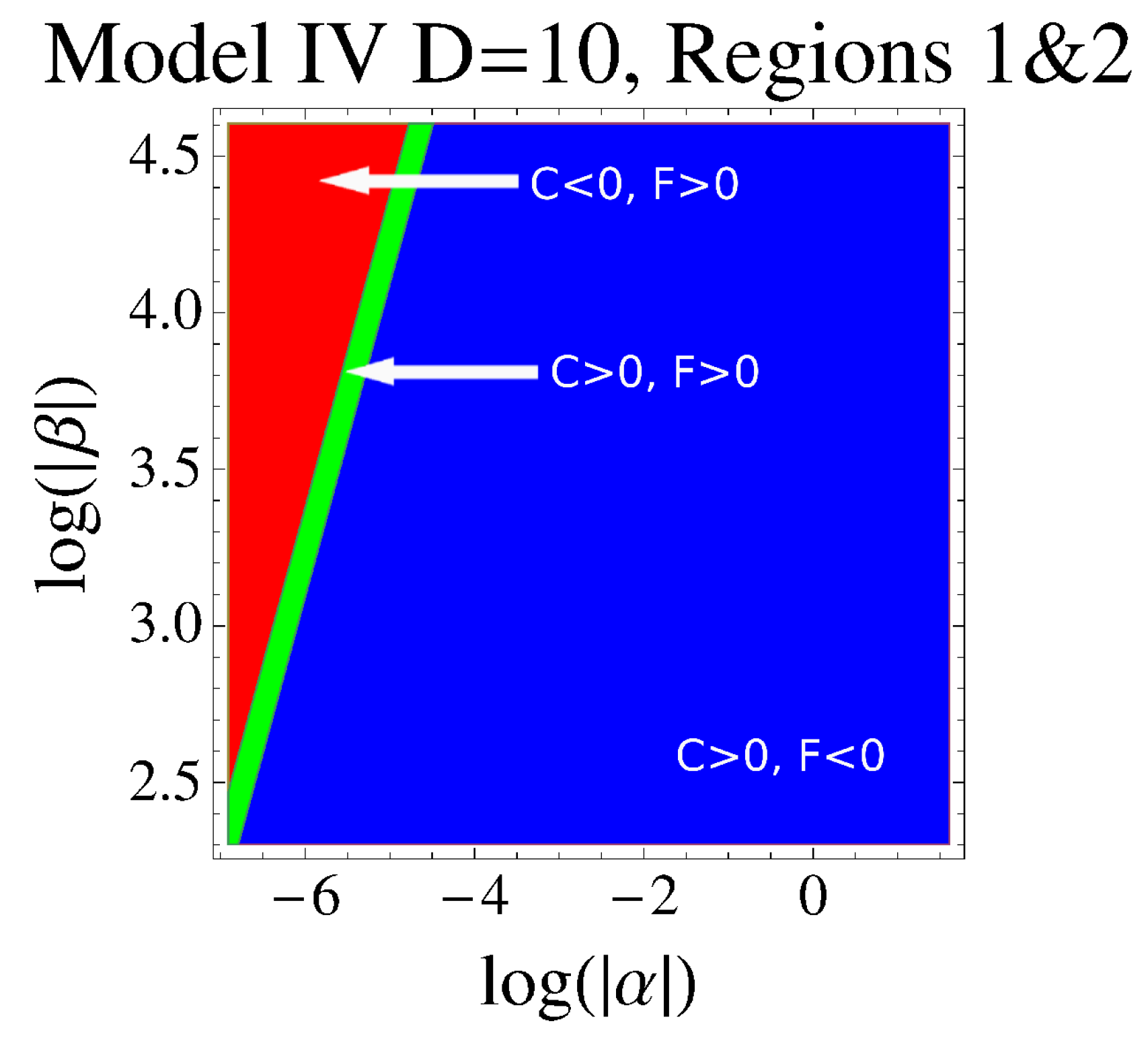
• Fast BH, with bigger values of the spin and the electric charge than the slow ones, shows a heat capacity always positive and a positive free energy up to a $M=M^{\mathit{\text{limit}}}$ value, and negative onwards. Thus, this BH is unstable against tunneling decay into radiation for mass parameter values of $M<M^{\mathit{\text{limit}}}$. For $M>M^{\mathit{\text{limit}}}$, free energy becomes negative, therefore smaller than that of pure radiation, that will tend to collapse to the BH configuration in equilibrium with thermal radiation.
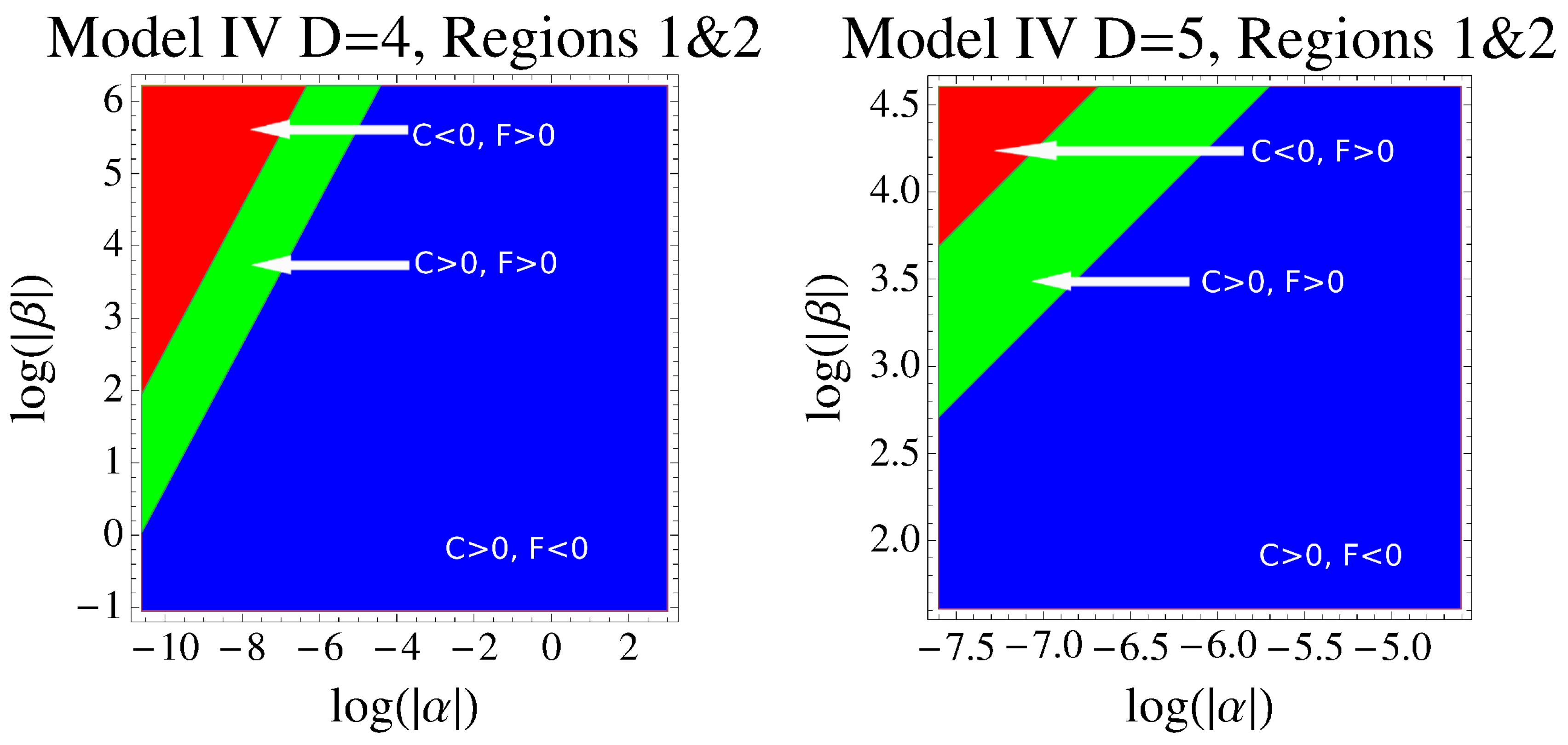
• Slow BH shows a more complex thermodynamics, being necessary to distinguish between four regions delimited by the mass parameter values: $M^{min}<M^{\mathrm{I}}<M^{\mathrm{II}}<M^{\mathit{\text{limit}}}$, as follows:

  −

  For $M^{min}<M<M^{\mathrm{I}}$ and for $M^{\mathrm{II}}<M<M^{\mathit{\text{limit}}}$, both the heat capacity and the free energy are positive, which means that the BH is unstable and decays into radiation by tunneling.

  −

  If $M^{\mathrm{I}}<M<M^{\mathrm{II}}$, the heat capacity becomes negative but free energy remains positive, being therefore unstable and decays into pure thermal radiation or to larger values of mass.

  −

  Finally, for $M>M^{\mathit{\text{limit}}}$ the heat capacity is positive whereas the free energy is now negative, thus tending pure radiation to tunnel to the BH configuration in equilibrium with thermal radiation.

Let us conclude this section as we did the previous one, by emphasizing that, although not quantitatively, the thermodynamical behavior of KN–AdS BH in $f\left(R\right)$ modified gravity theories is qualitatively analogous to that of GR [130]. This was an original important result presented for the first time in [120,121]. In that investigation, authors proved that some thermodynamical quantities like the physical mass $\mathcal{M}$, the angular momentum J and the entropy S differ from those of GR by a $(1+f^{\prime }\left(R_0\right))$ factor. One might think that the free energy F and the heat capacity C also differ in that same multiplicative way, but because of the dependence with the normalized charge parameter $\overline{Q}$, this same term $(1+f^{\prime }\left(R_0\right))$ leads to a more complex deviation from the GR behavior.

6. Thermodynamics in AdS and Kerr–Newman: Particular Examples

6.1. Thermodynamics in AdS

In order to illustrate the calculations sketched in Section 5.1, let us consider some particular $f\left(R\right)$ models in whose heat capacity C and the free energy F will be determined that were originally studied in [112,113]. As was pointed out above, those two quantities provide the local and global stability of AdS BH. For the particular models that are studied below, the constant scalar curvature $R_0$ could be calculated exactly by using Equation (27). For the sake of simplicity the D-dimensional Schwarzschild radius in Equation (31) was taken as $R_S^{D-3}\equiv 2$. The models we have considered are the following.

6.1.1. Model I: $f\left(R\right)=\alpha {(-R)}^{\beta }$

This model has been widely studied because the $\alpha R^2$ term with $\alpha >0$ can account for the accelerated expansion of the Universe [131]. This model can also explain the observed temperature anisotropies observed in the CMB, and can become a viable alternative to scalar field inflationary models, since reheating after inflation would have its origin on the production of particles during the oscillation phase of the Ricci scalar [132]. For $\beta =2$, this model was recently pointed out [16,18] as a possible explanation to dark matter.

Substituting this model in Equation (27) for arbitrary dimension and by only considering non-vanishing curvature solutions, the found solution is:

$$\begin{array}{c}\hfill R_0=-{\left[\frac{2-D}{(2\beta -D)\alpha }\right]}^{1/(\beta -1)}\end{array}$$

(70)

For $D>2$, the condition $(2\beta -D)\alpha <0$ provides well-defined scalar curvatures $R_0$. Two separated regions have thus to be studied: Region 1 $\{\alpha <0,\beta >D/2\}$ and region 2 $\{\alpha >0,\beta <D/2\}$. For this model we also get:

$$\begin{array}{c}\hfill 1+f^{\prime }\left(R_0\right)=\frac{D(\beta -1)}{2\beta -D}\end{array}$$

(71)

Notice that in region 1, $1+f^{\prime }\left(R_0\right)>0$ for $D>2$, since in this case $\beta >1$ is straightforwardly accomplished. In region 2, we find that for $D>2$, the requirement $R_0+f\left(R_0\right)<0$, i.e., $1+f^{\prime }\left(R_0\right)>0$, fixes $\beta <1$, since this is the most stringent constraint over the parameter β in this region. Therefore the physical space of parameters in region 2 is restricted to be $\{\alpha >0,\beta <1\}$.

In Figure 4 and Figure 5, taken from [112,113], one can see the physical regions in the parameter space $(\alpha ,\beta )$ corresponding to the different signs of $(C,F)$.

Figure 4. Thermodynamical regions in the $\left(\right|\alpha |,|\beta \left|\right)$ plane for Model I in $D=4$ (left) and $D=5$ (right).

Figure 4. Thermodynamical regions in the $\left(\right|\alpha |,|\beta \left|\right)$ plane for Model I in $D=4$ (left) and $D=5$ (right).

Figure 5. Thermodynamical regions in the $\left(\right|\alpha |,|\beta \left|\right)$ plane for Model I in $D=10$.

Figure 5. Thermodynamical regions in the $\left(\right|\alpha |,|\beta \left|\right)$ plane for Model I in $D=10$.

6.1.2. Model II: ${\displaystyle f\left(R\right)=-\alpha \frac{{\displaystyle \kappa {\left(\frac{R}{\alpha }\right)}^n}}{{\displaystyle 1+\beta {\left(\frac{R}{\alpha }\right)}^n}}}$

This model has been proposed in [106] as cosmologically viable and has attracted a lot of attention in order to constrain its validity in different astrophysical and cosmological scenarios. Throughout this study, let us consider $n=1$ for the sake of simplicity. A vanishing curvature solution also appears in this model and the two nontrivial curvature solutions are given by [112,113]:

$$\begin{array}{c}\hfill R_0^{\pm }=\frac{\alpha \left[(\kappa -2)D+4\pm \sqrt{\kappa }\sqrt{\kappa D^2-8D+16}\right]}{2\beta (D-2)}\end{array}$$

(72)

where $\kappa >0$ and $\kappa >(8D-16)/D^2$ are required for real $R_0$ solutions. The corresponding $1+f^{\prime }\left(R_0\right)$ values for Equation (72) are:

$$\begin{array}{c}\hfill 1+f^{\prime }\left(R_0^{\pm }\right)=1-\frac{4{(D-2)}^2}{{\left(\sqrt{\kappa D^2-8D+16}\pm \sqrt{\kappa }D\right)}^2}\end{array}$$

(73)

Since $1+f^{\prime }\left(R_0\right)>0$ is required, one has $\text{sign}\left(R_0^{\pm }\right)=\text{sign}\left(\alpha \beta \right)$. In fact it turns out that $1+f^{\prime }\left(R_0^{-}\right)$ is not positive for any allowed value of κ and therefore this curvature solution $R_0^{-}$ is excluded for our study (see [112,113] for details). On the other hand, $1+f^{\prime }\left(R_0^{+}\right)>0$ only requires $\kappa >0$ for dimension $D\ge 4$ and therefore $f^{\prime }\left(R_0\right)<0$. Therefore only two accessible regions need to be studied: region 1 $\{\alpha >0,\beta <0\}$ and region 2, $\{\alpha <0,\beta >0\}$.

6.2. KN–AdS Thermodynamics

In this section we will study the thermodynamics of the two $f\left(R\right)$ models presented in the last section but when a Kerr–Newman configuration is considered.

First, as was shown above, the condition $1+f^{\prime }\left(R_0\right)>0$ must be satisfied in order to obtained physical results, so first of all the viability of each model depending upon the values of the parameters that define them will be checked out. Thus, for each model, we will study the range of parameters that allows the existence of Kerr–Newman BH, i.e., we will graphically display $a_{max}$ and $a_{min}$ (if present) in terms of those parameters, and study the region of a confined between these two surfaces. This phenomenology was absent in the SAdS study since the configuration was spherically symmetric and therefore $a=0$. Finally we will focus on the thermodynamical quantities that define BH stability depending again upon the model range of parameters. In order to sketch graphically the thermodynamical behavior, let us then consider the BH parameter values: $M=1$, $a=0.4$ and $\overline{Q}=0.2$. Let us remind at this stage that this analysis is restricted to $R_0<0$ condition, as explained in the beginning of Section 5.

For the sake of simplicity, let us introduce the dimensionless variables notation [120,121] that we will use in the graphical visualization of the results to be presented:

$$\begin{array}{c}\hfill \frac{r}{M}\to r,\frac{a}{M}\to a,\frac{\overline{Q}}{M}\to \overline{Q},R_0{M}^2\to R_0\end{array}$$

(74)

where the previous symbols keep their original meaning as defined before. The considered models are as follows.

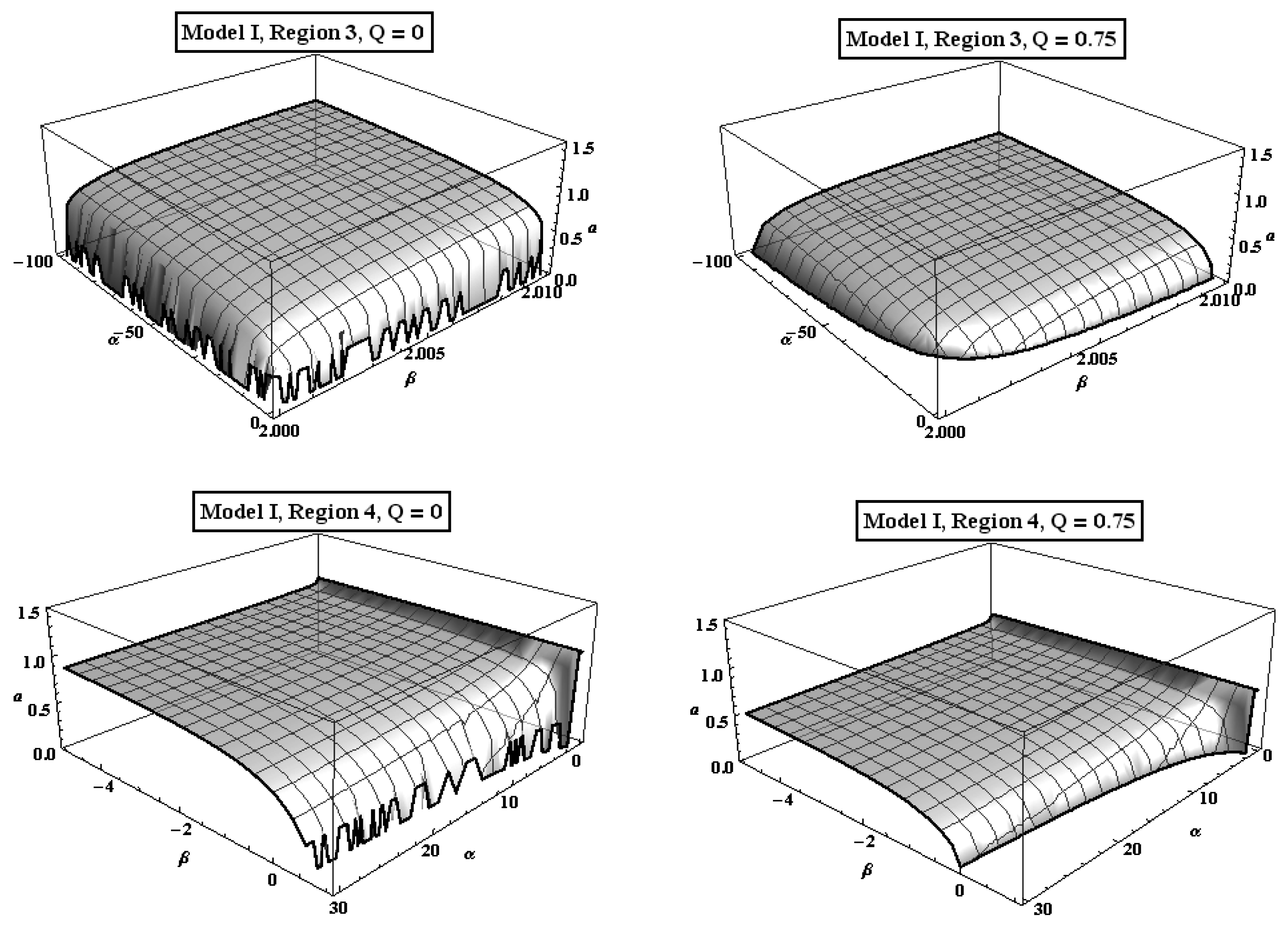
6.2.1. Model I: $f\left(R\right)=\alpha {(-R)}^{\beta }$

Let us remind the solution Equation (70) found above for this model. The viability condition $1+f^{\prime }\left(R_0^{}\right)>0$ restricts the range of parameters that define this $f\left(R\right)$ model.

In Figure 6, we show the range of the spin parameter a for which BH are allowed, depending on the parameters α and β and for charge parameters values $Q=0$ and $Q=0.75$. For the solution $R_0<0$ there exist two possible regions:

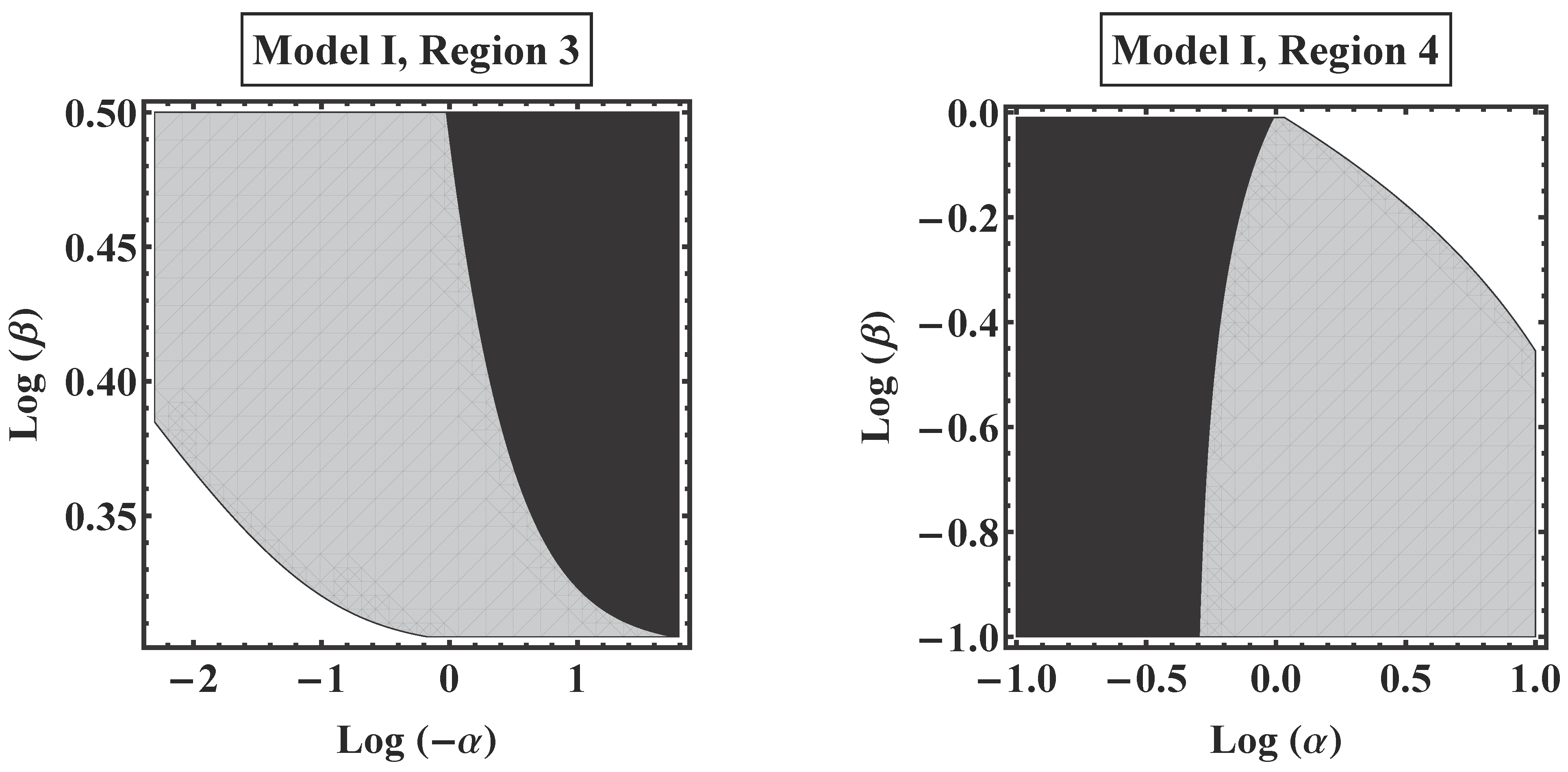
• Region 3 $\left\{\alpha <0,\beta >2\right\}$. For this region, the value of $a_{max}$ decreases suddenly from its normal value to 0 near the frontier of the region, i.e., $\alpha \approx 0$ and $\beta \approx 2$; other values of α and β display a relatively low curvature and the existence of BH is assured.
• Region 4 $\left\{\alpha >0,\beta <1\right\}$. This region only shows problems when $0<\beta <1$, where $a_{max}\to 0$, but, as β becomes more negative, the surface of $a_{max}$ slowly acquires higher values, recovering its usual value for $\beta =-2$.

Figure 6. Model I: Region 3: $\left\{\alpha <0,\beta >2\right\}$, and Region 4: $\left\{\alpha >0,\beta <1\right\}$. BH with a well defined horizon structure will only exist if they have a spin parameter below the upper surface $a_{max}$. For the presented regions 3 and 4, the surface $a_{min}$ does not exist.

Figure 6. Model I: Region 3: $\left\{\alpha <0,\beta >2\right\}$, and Region 4: $\left\{\alpha >0,\beta <1\right\}$. BH with a well defined horizon structure will only exist if they have a spin parameter below the upper surface $a_{max}$. For the presented regions 3 and 4, the surface $a_{min}$ does not exist.

We have graphically schematized in Figure 7 the possible thermodynamical configurations of a BH for Regions 3 and 4, i.e., $R_0<0$ following the results presented in [120,121]. As we can see in Region 3, only for values close to the region boundary ($\alpha \approx 0$ and $\beta \approx 2$) is BH stable both locally and globally ($C>0$ and $F<0$). Also, as the absolute value of α increases, it is more probable that the BH shows global instability ($C>0$ and $F>0$) and finally global and local instability ($C<0$ and $F>0$). In Region 4, however, we find the opposite behavior: near the limit of the region values ($\alpha \approx 0$ and $\beta \approx 1$) we have global and local instability, and, as α gets bigger, the BH becomes more stable both locally and globally.

Figure 7. Thermodynamical regions for Model I. We distinguish between three different regions: (i) $C<0$ and $F>0$, in black; (ii) $C>0$ and $F>0$, in gray; (iii) $C>0$ and $F<0$, in white.

Figure 7. Thermodynamical regions for Model I. We distinguish between three different regions: (i) $C<0$ and $F>0$, in black; (ii) $C>0$ and $F>0$, in gray; (iii) $C>0$ and $F<0$, in white.

6.2.2. Model II: ${\displaystyle f\left(R\right)=-\alpha \frac{{\displaystyle \kappa {\left(\frac{R}{\alpha }\right)}^n}}{{\displaystyle 1+\beta {\left(\frac{R}{\alpha }\right)}^n}}}$

Let us consider for the sake of simplicity again $n=1$, thus having a two-parameters model, since we can define $\gamma =\beta /\alpha$ and then obtain:

$$\begin{array}{c}\hfill f\left(R\right)=-\frac{\kappa R}{1+\gamma R}\end{array}$$

(75)

Replacing the latter in Equation (27), one gets Equation (72), that for $D=4$, and focusing on the negative constant curvature solution, yields:

$$\begin{array}{c}\hfill R_0^{}=-\frac{1-\kappa }{\gamma }-\sqrt{\frac{-\kappa (1-\kappa )}{{\gamma }^2}},\end{array}$$

(76)

Keeping in mind that we have to satisfy $1+f^{\prime }\left(R_0\right)>0$, κ happens to be restricted to values of $\kappa >1$. On the other hand, computation of $1+f^{\prime }\left(R_0\right)$ reveals that $R_0$ is only a valid solution for values of κ and γ in the Region 2: $\{\kappa >1,\gamma <0\}$, being as mentioned $R_0<0$. In Figure 8 we show the range of the spin parameter a for which BH are allowed, depending on the parameters κ and γ for certain values of the charge $\overline{Q}$. Region 2 displays an $a_{max}$ surface that descends slightly as the value of κ increases, and more significantly when $\gamma \approx 0$, becoming 0 when this limit is reached.

We graphically schematize in Figure 9 the different possible thermodynamical configurations for the region in which $R_0<0$, in this case the region 2. In this parameter space region, a combination of high values of κ and small absolute values of γ favor BH local and global stability, and, conversely, a combination of small values of κ and high absolute values of γ lead to BH instability, first globally and then also locally.

Figure 8. Model II. Region 1: $\left\{\kappa >1,\gamma >0\right\}$, and Region 2: $\left\{\kappa >1,\gamma <0\right\}$. BH with a well-defined horizon structure will only exist if they have a spin parameter below the upper surface $a_{max}$, and above a second surface $a_{min}$ (in case it exists, only in region 1 for this model) for certain values of κ and γ.

Figure 8. Model II. Region 1: $\left\{\kappa >1,\gamma >0\right\}$, and Region 2: $\left\{\kappa >1,\gamma <0\right\}$. BH with a well-defined horizon structure will only exist if they have a spin parameter below the upper surface $a_{max}$, and above a second surface $a_{min}$ (in case it exists, only in region 1 for this model) for certain values of κ and γ.

Figure 9. Thermodynamical regions with negative scalar curvature $R_0<0$ of model I. We distinguish between three different regions: (i) $C<0$ and $F>0$, in black; (ii) $C>0$ and $F>0$, in gray; (iii) $C>0$ and $F<0$, in white.

Figure 9. Thermodynamical regions with negative scalar curvature $R_0<0$ of model I. We distinguish between three different regions: (i) $C<0$ and $F>0$, in black; (ii) $C>0$ and $F>0$, in gray; (iii) $C>0$ and $F<0$, in white.

7. Cosmological Solutions in Modified Gravity

Modified gravity has become very popular in recent years because it is capable to reproduce the dark energy epoch, and even the inflationary phase, with no need to introduce an additional component in the universe. Hence, the reconstruction of appropriate theories that contain some particular cosmological solutions have involved an important effort (see [37,38,42,43,44,45,46,101,133,134,135,136,137,138,139,140,141,142,143,144,145,146,147,148,149]). The same is true for the reconstruction of so-called viable modified gravities, which can recover GR in some limit while they introduce additional effects at cosmological scales (see [106,107,108,109,110]). However, as in every dark energy model, the required fine tuning on the form of the action as on free parameters of the model have resulted in a large effort in searching additional and independent predictions in the frame of modified gravities, including other aspects different than cosmology as the ones studied in the above sections (see also the reviews [26,27,28,29,30,31,32,33] and references therein). In this section we are interested to make a short review on cosmological solutions in the frame of modified gravities, and in particular in $F\left(R\right)$ gravity, while the thermodynamical aspects are studied in the following sections. As it is widely accepted, our universe seems to be well described by FLRW metrics:

$$d{s}^2=-d{t}^2+a^2\left(t\right)\left[\frac{1}{1-k{r}^2}d{r}^2+r^{2}d{\theta }^2+r^2{sin}^2\theta d{\phi }^2\right]$$

(77)

and specifically the universe seems to be spatially flat, $k=0$. Hence, by introducing the metric in $F\left(R\right)$ field Equation (3), modified FLRW equations are obtained:

$$\begin{array}{c}\hfill H^2=\frac{1}{3F_R}\left[{\kappa }^2{\rho }_m+\frac{R{F}_R-F}{2}-3H\dot{R}{F}_{RR}\right]\\ \hfill -3H^2-2\dot{H}=\frac{1}{F_R}\left[{\kappa }^2{p}_m+{\dot{R}}^2{F}_{RRR}+2H\dot{R}{F}_{RR}+\ddot{R}{F}_{RR}+\frac{1}{2}(F-R{F}_R)\right]\end{array}$$

(78)

Recent astronomical data indicates that the well-known ΛCDM model where DE is represented by an effective cosmological constant fits quite well the observational data. Nevertheless, it is shown that $F\left(R\right)$ gravity can even reproduce exactly the ΛCDM model in absence of a cosmological constant s shown below (see [37,150]). Let us consider ΛCDM cosmology:

$$\frac{3}{{\kappa }^2}{H}^2=\frac{3}{{\kappa }^2}{H}_0^2+{\rho }_0{a}^{-3}=\frac{3}{{\kappa }^2}{H}_0^2+{\rho }_0{a}_0^{-3}{\mathrm{e}}^{-3N}$$

(79)

where we have introduced the number of e-foldings $N=ln\frac{a}{a_0}$ instead of the cosmological time t, and we have assumed a pressureless fluid. We can easily solve the continuity equation for ${\rho }_m$:

$$\dot{\rho }+3H(1+w_m)\rho =0$$

(80)

while the first FLRW equation in Equation (78) can be rewritten in terms of the number of e-foldings, which yields [148]:

$$\begin{array}{ccc}\hfill 0& =& -9G\left(N\left(R\right)\right)\left(4G^{\prime }\left(N\left(R\right)\right)+G^{″}\left(N\left(R\right)\right)\right)\frac{d^{2}F\left(R\right)}{d{R}^2}+\left(3G\left(N\left(R\right)\right)+\frac{3}{2}{G}^{\prime }\left(N\left(R\right)\right)\right)\frac{dF\left(R\right)}{dR}\hfill \\ & & -\frac{F\left(R\right)}{2}+\sum _i{\rho }_{i0}{a}_0^{-3(1+w_i)}{\mathrm{e}}^{-3(1+w_i)N\left(R\right)}\hfill \end{array}$$

(81)

where $G\left(N\right)=H^2$. Hence, for ΛCDM cosmology Equation (79), the scalar curvature is given by $R=3G^{\prime }\left(N\right)+12G\left(N\right)=12H_0^2+{\kappa }^2{\rho }_0{a}_0^{-3}{\mathrm{e}}^{-3N}$, and the Equation (81) gives a hypergeometric equation [37]:

$$0=3\left(R-9H_0^2\right)\left(R-12H_0^2\right)\frac{d^{2}F\left(R\right)}{d^{2}R}-\left(\frac{1}{2}R-9H_0^2\right)\frac{dF\left(R\right)}{dR}-\frac{1}{2}F\left(R\right)$$

(82)

whose solution is given by:

$$F\left(x\right)=AF(\alpha ,\beta ,\gamma ;x)+B{x}^{1-\gamma }F(\alpha -\gamma +1,\beta -\gamma +1,2-\gamma ;x)$$

(83)

where $x=\frac{R}{3H_0^2}-3$, $\{A,B\}$ are integration constants, and the parameters are:

$$\gamma =-\frac{1}{2},\alpha +\beta =-\frac{1}{6},\alpha \beta =-\frac{1}{6}$$

(84)

Hence, the action Equation (83) is capable to reproduce ΛCDM model with no cosmological constant. Nevertheless, the action Equation (83) is composed by hypergeometric functions, which do not seem to provide a successful explanation for dark energy, since the theory turns out much complicated than the usual GR with a cosmological constant. However, other viable models of $F\left(R\right)$ gravity capable to mimic a cosmological constant at the present time have been suggested in the literature (see [106,107,108,109,110]), which in general seem to cross the phantom barrier [151]. Then, let us now study a model where the dominant component is phantom-like. Such kind of system can be easily expressed in the standard General Relativity when a phantom fluid is considered, where the FLRW equation reads $H^2\left(t\right)=\frac{{\kappa }^2}{3}{\rho }_{\mathrm{ph}}$ (the subscript $ph$ denotes the phantom nature of the fluid). As the EoS for the fluid is given by $p_{\mathrm{ph}}=w_{\mathrm{ph}}{\rho }_{\mathrm{ph}}$ with $w_{\mathrm{ph}}<-1$, by using the conservation equation, the solution yields $a\left(t\right)=a_0{(t_s-t)}^{-H_0}$, where $a_0$ is a constant, $H_0=-\frac{1}{3(1+w_{\mathrm{ph}})}$ and $t_s$ is the so-called Rip time. Then, the solution describes a universe that ends in a Big Rip singularity at the time $t_s$. The same behavior can be achieved in $F\left(R\right)$ theory with no need to introduce a phantom fluid. The expression for the Hubble parameter as a function of the number of e-foldings is given by $H^2\left(N\right)=H_0^2{\mathrm{e}}^{2N/H_0}$. Then, the Equation (81), with no matter contribution, takes the form:

$$R^2\frac{d^{2}F\left(R\right)}{d{R}^2}+AR\frac{dF\left(R\right)}{dR}+BF\left(R\right)=0$$

(85)

where $A=-H_0(1+H_0)$ and $B=\frac{(1+2H_0)}{2}$. This equation is an Euler equation whose solution yields:

$$F\left(R\right)=C_1{R}^{m_{+}}+C_2{R}^{m_{-}},\text{where}{m}_{\pm }=\frac{1-A\pm \sqrt{{(A-1)}^2-4B}}{2}$$

(86)

Thus, the phantom cosmology $a\left(t\right)=a_0{(t_s-t)}^{-H_0}$ can be also obtained in the frame of $F\left(R\right)$ theory and no phantom fluid is needed.

In addition, the equivalence between $f\left(R\right)$ gravity and scalar-tensor theories Equation (4) can be used to easily obtain cosmological solutions in $f\left(R\right)$ gravity. For the metric Equation (77), Friedmann equations read:

$$\begin{array}{c}\hfill 3H\frac{dP\left(\varphi \right)}{dt}+3H^{2}P\left(\varphi \right)+\frac{1}{2}Q\left(\varphi \right)-{\rho }_m=0\end{array}$$

$$\begin{array}{c}\hfill \frac{d^{2}P\left(\varphi \right)}{d{t}^2}+2H\frac{dP\left(\varphi \right)}{dt}+(2\dot{H}+3H^2)P\left(\varphi \right)+\frac{1}{2}Q\left(\varphi \right)+p_m=0\end{array}$$

(87)

We redefine the scalar field such that it is chosen to be the time coordinate $\varphi =t$. Hence, taking into account the Equations (87) and the continuity equation for the perfect fluid ${\rho }_m$, the Hubble parameter may be calculated as a function of the scalar field φ, $H=g\left(\varphi \right)$. By combining the Equation (87), the function $Q\left(\varphi \right)$ is deleted, and it yields:

$$\frac{d^{2}P\left(\varphi \right)}{d{\varphi }^2}-g\left(\varphi \right)\frac{dP\left(\varphi \right)}{d\varphi }+2g^{\prime }\left(\varphi \right)P\left(\varphi \right)+(1+w_m){\rho }_{m0}exp\left[-3(1+w_m)\int d\varphi g\left(\varphi \right)\right]=0$$

(88)

By solving this equation for a given function $P\left(\varphi \right)$, a cosmological solution $H\left(t\right)$ is found, and the function $Q\left(\varphi \right)$ is obtained by means of equations in Equation (87):

$$Q\left(\varphi \right)=-6{\left(g\left(\varphi \right)\right)}^{2}P\left(\varphi \right)-6g\left(\varphi \right)\frac{dP\left(\varphi \right)}{d\varphi }+2{\rho }_{m0}exp\left[-3(1+w_m)\int d\varphi g\left(\varphi \right)\right]$$

(89)

If we neglect the contribution of matter, then the Equation (88) is a first order differential equation on $g\left(\varphi \right)$, and it can be easily solved. The solution found is the following [147]:

$$g\left(\varphi \right)=C\sqrt{P\left(\varphi \right)}-\sqrt{P\left(\varphi \right)}\int d\varphi \frac{P^{″}\left(\varphi \right)}{2P^{3/2}\left(\varphi \right)}$$

(90)

where C is an integration constant. Hence, we have shown that $F\left(R\right)$ gravity represents a serious candidate to explain the phenomena of late-time acceleration in the expansion of the universe. In the following sections, we explore the thermodynamical properties of FLRW metrics in the frame of modified gravity as well as an attempt to generalize Cardy–Verlinde formula.

8. First Law of Thermodynamics and FLRW Equations

In this section, we review some of the most important results obtained in the study of FLRW metrics and their thermodynamics, specifically the relation between the first law of thermodynamics and FLRW equations, which can be deduced by assuming the well known relation between the entropy and the horizon area, as well as the relation between the gravity surface and the temperature [82,83,84]. Such study has been extended not only to $f\left(R\right)$ gravity, as is also shown below (see [85]), but also to many other different scenarios [86,87,88,89,90,91,92,93,94,95,96]. In fact, it was found in [80] and extended in [81] for $f\left(R\right)$ gravities, a direct deduction of gravity field equations by assuming the relation of the horizon area and the entropy. Nevertheless, here we are only interested to show the deduction of FLRW equation from the thermodynamics defined in the corresponding horizons of a particular spacetime. Let us consider a $n+1$ FLRW metric Equation (77), with arbitrary spatial curvature $k=-1,0,1$. This metric may be rewritten as:

$$d{s}^2=h_{ab}d{x}^{a}d{x}^b+{\tilde{r}}^{2}d{\Omega }_{n-1}^2$$

(91)

where the indexes $a,b=0,1$, being $x^0=t$, $x^1=r$, and $\tilde{r}=a\left(t\right)r$, while $d{\Omega }_{n-1}^2$ expresses the line element of an $n-1$ unit sphere. Then, the apparent horizon for this general kind of spacetimes is defined as $h^{ab}{\partial }_a\tilde{r}{\partial }_b\tilde{r}=0$, whose radius yields:

$${\tilde{r}}_A=\frac{1}{\sqrt{H^2+k/a^2}}$$

(92)

As will be shown below, one can assign an entropy proportional to the area of the apparent horizon as well as an energy flux through the horizon. This is the reason for considering the apparent horizon instead of other horizons defined in FLRW spacetimes. We may define the work density and the energy flux vector as [82,83,84]:

$$\begin{array}{c}\hfill w=-h_{ab}{T}^{ab},\end{array}$$

(93)

$$\begin{array}{c}\hfill {\Psi }_a=T_a^b{\partial }_b\tilde{r}+w{\partial }_a\tilde{r}\end{array}$$

(94)

where the work w refers to the change experimented by the apparent horizon, while the vector ${\Psi }_a$ refers to the flux of energy through the horizon. Then, the variation of the internal energy can be written as:

$$\overrightarrow{\nabla }E=A\overrightarrow{\Psi }+w\overrightarrow{\nabla }V$$

(95)

where A is the area and V is the volume of an n-dimensional space with radius $\tilde{r}$. This equation represents the unified first law according to [152]. The first term in the r.h.s. in Equation (95) takes the form:

$$A\overrightarrow{\Psi }=\frac{\kappa }{8\pi G}\overrightarrow{\nabla }A+{\tilde{r}}^{n-2}\overrightarrow{\nabla }\left(\frac{E}{{\tilde{r}}^{n-2}}\right)$$

(96)

where κ is the surface gravity:

$$\kappa =\frac{1}{\sqrt{-h}}{\partial }_a\left(\sqrt{-h}{h}^{ab}{\partial }_b\tilde{r}\right)$$

(97)

Note that the energy is defined as:

$$E=\frac{n(n-1){\Omega }_n}{16\pi G}{\tilde{r}}^{n-2}(1-h^{ab}{\partial }_a\tilde{r}{\partial }_b\tilde{r})$$

(98)

Hence at the apparent horizon, the second term in the r.h.s. in Equation (96) vanishes, as on the black hole event horizon, so that the expression Equation (96) can be identified with the thermodynamical relation $dE=-TdS$ if the surface gravity is assumed to be the temperature $\kappa /2\pi$, and the entropy yields the usual expression, proportional to $A/4G$. Now if we assume a perfect fluid filling the universe, with an energy-momentum tensor given by $T_{\mu \nu }=(\rho +p)u_{\mu }{u}_{\nu }+p{g}_{\mu \nu }$, the energy flux vector yields:

$$\overrightarrow{\Psi }=\left(-\frac{1}{2}(\rho +p)H\tilde{r},\frac{1}{2}(\rho +p)a\right)$$

(99)

Then, the change of the internal energy through the apparent horizon Equation (96) becomes:

$$dE=A\Psi =-A(\rho +p)H{\tilde{r}}_{A}dt$$

(100)

Identifying the entropy and temperature associated to the apparent horizon,

$$S=\frac{A}{4G},T=\frac{1}{2\pi {\tilde{r}}_A}$$

(101)

and using the first law of thermodynamics $dE=-TdS$, the second FLRW equation is obtained:

$$\dot{H}=-\frac{8\pi G}{n-1}(\rho +p)+\frac{k}{a^2}$$

(102)

By combining it with the continuity Equation (80), the first FLRW equation is also obtained. Hence, FLRW equations can be deduced by using only thermodynamical arguments and identifying the entropy of the apparent horizon and its temperature, which is an identity that supports the idea of the relation between gravitational field equations and thermodynamical ones, as suggested by Jacobson in [80].

In the same way, this analysis can be easily extended to $f\left(R\right)$ gravity as well as to other modified theories of gravity. Specifically, for $F\left(R\right)$ gravity, the entropy relation is defined (see previous sections) as follows:

$$S=\frac{A{F}^{\prime }\left(R\right)}{4G}$$

(103)

Hence, following the same steps performed above for GR, the FLRW equations for $f\left(R\right)$ gravity Equation (78) are recovered [85]. Then, a strong relation between thermodynamics of the horizons and gravitational field equations is established. In the next section, another aspect of the relation of FLRW equations and thermodynamics is explored, in that case following the holographic principle through the entropy bounds and the Cardy–Verlinde formula.

9. Generalization of Cardy–Verlinde Formula

This section is devoted to consideration of the Cardy–Verlinde formula for general scenarios, and in particular for modified gravity. The Cardy–Verlinde formula was established by Verlinde in [98] as a thermodynamical relation between FLRW equations with a conformal fluid (a radiation-like fluid) and the Cardy formula (see [97]), and it was extended for a general perfect fluid in [99]. In [100], attempts to reproduce the Cardy–Verlinde formula was suggested for different scenarios, including modified gravity. Other aspects of the Cardy–Verlinde formula such as the presence of a viscous fluid have been studied in [153,154,155]. In this section, we mainly review those results. We consider a $(n+1)$-dimensional spacetime described by the FLRW metric Equation (77). By inserting the metric Equation (77) in the Einstein field equations, the FLRW equations for GR are derived:

$$H^2=\frac{16\pi G}{n(n-1)}\sum _{i=1}^m{\rho }_i-\frac{k}{a^2},\dot{H}=-\frac{8\pi G}{n-1}\sum _{i=1}^m({\rho }_i+p_i)+\frac{k}{a^2}$$

(104)

Here ${\rho }_i=E_i/V$ and $p_i$ are the energy-density and pressure of the matter component i that fills the Universe. In this section, we consider only the $k=1$ closed Universe. Moreover, we assume an equation of state (EoS) of the form $p_i=w_i{\rho }_i$ with $w_i$ constant for each fluid, and assume no interaction between the different components. Then, the continuity Equation (80) has the form now $\dot{{\rho }_i}+nH\left({\rho }_i+p_i\right)=0$ and by solving it, we find that the i fluid depends on the scale factor as:

$${\rho }_i\propto a^{-n(1+w_i)}$$

(105)

Let us now review the case of [99], where just one fluid with EoS $p=w\rho$ and $w=\text{constant}$ is considered. The total energy inside the comoving volume V, $E=\rho V$, can be written as the sum of an extensive part $E_{\mathrm{E}}$ and a subextensive part $E_{\mathrm{C}}$, called the Casimir energy (for other ways to account the Casimir energy in a FLRW universe, see [156,157]), and takes the form:

$$E(S,V)=E_{\mathrm{E}}(S,V)+\frac{1}{2}{E}_{\mathrm{C}}(S,V)$$

(106)

Under a rescaling of the entropy ($S\to \lambda S$) and the volume ($V\to \lambda V$), the extensive and subextensive parts of the total energy transform as:

$$E_{\mathrm{E}}(\lambda S,\lambda V)=\lambda E_{\mathrm{E}}(S,V),E_{\mathrm{C}}(\lambda S,\lambda V)={\lambda }^{1-2/n}{E}_{\mathrm{C}}(S,V)$$

(107)

Hence, by assuming that the Universe satisfies the first law of thermodynamics, the term corresponding to the Casimir energy $E_{\mathrm{C}}$ can be seen as a violation of the Euler identity according to the definition in [98]:

$$E_{\mathrm{C}}=n(E+pV-TS)$$

(108)

Since the total energy behaves as $E\sim a^{-nw}$ and by the definition Equation (106), the Casimir energy also goes as $E_{\mathrm{C}}\sim a^{-nw}$. The FLRW universe expands adiabatically, $dS=0$, so the products $E_{\mathrm{C}}{a}^{nw}$ and $E_{\mathrm{E}}{a}^{nw}$ should be independent of the volume V, and be just a function of the entropy. Then, by the rescaling properties Equation (107), the extensive and subextensive part of the total energy can be written as functions of the entropy only [99]:

$$E_{\mathrm{E}}=\frac{\alpha }{4\pi a^{nw}}{S}^{w+1},E_{\mathrm{C}}=\frac{\beta }{2\pi a^{nw}}{S}^{w+1-2/n}$$

(109)

Here α and β are undetermined constants. By combining these expressions with Equation (106), the entropy of the Universe is written as a function of the total energy E and the Casimir energy $E_{\mathrm{C}}$ [99]:

$$S={\left(\frac{2\pi a^{nw}}{\sqrt{\alpha \beta }}\sqrt{E_{\mathrm{C}}(2E-E_{\mathrm{C}})}\right)}^{\frac{n}{n(w+1)-1}}$$

(110)

which for $w=1/n$ (radiation-like fluid) reduces to [98]:

$$S=\frac{2\pi a}{\sqrt{\alpha \beta }}\sqrt{E_{\mathrm{C}}(2E-E_{\mathrm{C}})}$$

(111)

which has the same form as the Cardy formula given in [97]. The first FLRW Equation (104) can be rewritten as a relation between thermodynamics variables, and yields:

$$S_{\mathrm{H}}=\frac{2\pi }{n}a\sqrt{E_{\mathrm{BH}}(2E-E_{\mathrm{BH}})},\mathrm{where}{S}_{\mathrm{H}}=(n-1)\frac{HV}{4G},E_{\mathrm{BH}}=n(n-1)\frac{V}{8\pi G{a}^2}.$$

(112)

It is easy to check that for the bound proposed in [98], $E_{\mathrm{C}}\le E_{\mathrm{BH}}$, the equation for the entropy Equation (111) coincides with the first FLRW Equation (112) when the bound is reached. We will see below that when there are several fluid components, the same kind of expression as in [98] cannot be found as well as its extension to modified gravity, nor is there the same correspondence with the FLRW equation when the bound is saturated.

9.1. Multicomponent Universe

If m fluids are considered with arbitrary EoS, $p_i=w_i{\rho }_i$, the expression for the total entropy is simple to derive just by following the same method as above. The total entropy is given by the sum of the entropies for each fluid [100]:

$$S=\sum _{i=1}^m{S}_i=\sum _{i=1}^m{\left(\frac{2\pi a^{n{w}_i}}{\sqrt{\alpha \beta }}\sqrt{E_{iC}(2E_i-E_{iC})}\right)}^{\frac{n}{n(w_i+1)-1}}$$

(113)

This expression cannot be reduced to one depending only on the total energy unless very special conditions on the nature of the fluids are assumed. Let us for simplicity assume that there are only two fluids with EoS given by $p_1=w_1{\rho }_1$ and $p_2=w_2{\rho }_2$, $w_1$ and $w_2$ being constants. We can substitute the fluids by an effective fluid described by the EoS:

$$p_{\mathrm{eff}}=w_{\mathrm{eff}}{\rho }_{\mathrm{eff}},\text{where}{w}_{\mathrm{eff}}=\frac{p_1+p_2}{{\rho }_1+{\rho }_2}=w_1+\frac{w_2-w_1}{1+{\rho }_1/{\rho }_2}$$

(114)

and $p_{\mathrm{eff}}=\frac{1}{2}(p_1+p_2)$, ${\rho }_{\mathrm{eff}}=\frac{1}{2}({\rho }_1+{\rho }_2)$. Then, by using the energy conservation Equation (80), we find ${\rho }_1\sim {(a/a_0)}^{-n(1+w_1)}$ and ${\rho }_2\sim {(a/a_0)}^{-n(1+w_2)}$, where $a_0$ is assumed to be the value of the scale factor at the time $t_0$. The effective EoS parameter $w_{\mathrm{eff}}$ can be expressed as a function of the scale factor $a\left(t\right)$:

$$w_{\mathrm{eff}}=w_1+\frac{w_2-w_1}{1+{(a/a_0)}^{n(w_2-w_1)}}$$

(115)

The total energy inside a volume V becomes:

$$E_T=E_1+E_2\propto {(a/a_0)}^{-n{w}_1}+{(a/a_0)}^{-n{w}_2}$$

(116)

As the energy is proportional to two different powers of the scale factor a, it is not possible to write it as a function of the total entropy only. As a special case, if the EoS parameters are $w_1=w_2=w_{\mathrm{eff}}$, the formula for the entropy reduces to Equation (110), and coincides with the CV formula when $w_{\mathrm{eff}}=1/n$.

As another case, one might consider that for some epoch of the cosmic history, $w_1\gg w_2$. Taking also $a>>a_0$, we could then approximate the total energy by the function $E_T\propto a^{-n{w}_2}$. From Equation (106) the Casimir energy would also depend on the same power of a, $E_{\mathrm{C}}\propto a^{-n{w}_2}$. The expression Equation (110) is again recovered with $w=w_2$.

Thus in general, when a multicomponent FLRW Universe is assumed, the formula for the total entropy does not resemble the Cardy formula, nor does it correspond to the FLRW equation when the Casimir bound is reached. It becomes possible to reconstruct the formula Equation (111), and establish the correspondence with the Cardy formula, only if we make specific choices for the EoS of the fluids.

9.2. Inhomogeneous EoS Fluid and Modified Gravity

Let us now explore the case of an $n+1$-dimensional Universe filled with a fluid satisfying an inhomogeneous EoS. This kind of EoS, generalizing the perfect fluid model, has been considered in several papers as a way to describe effectively the DE (see [158,159]). We assume an EoS expressed as a function of the scale factor:

$$p=w\left(a\right)\rho +g\left(a\right)$$

(117)

This EoS fluid could be taken to correspond to modified gravity, or to bulk viscosity [158,159]. By introducing Equation (117) in the energy conservation Equation (80) we obtain:

$${\rho }^{\prime }\left(a\right)+\frac{n(1+w(a\left)\right)}{a}\rho \left(a\right)=-n\frac{g\left(a\right)}{a}$$

(118)

Here we have performed a variable change $t=t\left(a\right)$ such that the prime over ρ denotes derivative with respect to the scale factor a. The general solution of this equation is:

$$\rho \left(a\right)={\mathrm{e}}^{-F\left(a\right)}\left(C-n\int {\mathrm{e}}^{F\left(a\right)}\frac{g\left(a\right)}{a}da\right)\text{where}F\left(a\right)={\int }^a\frac{1+w\left(a^{\prime }\right)}{a^{\prime }}d{a}^{\prime }$$

(119)

and C is an integration constant. As shown above, only for some special choices of the functions $w\left(a\right)$ and $g\left(a\right)$ can the formula Equation (111) be recovered. Let us assume, as an example, that $w\left(a\right)=-1$ and $g\left(a\right)=-a^m$, with m being constant. Then, the energy density behaves as $\rho \propto a^m$. Hence, by following the same steps as described above, the extensive and subextensive energy go as $a^{m+n}$, and by imposing conformal invariance and the rescaling properties Equation (107), we calculate the dependence on the entropy to be:

$$E_{\mathrm{E}}=\frac{\alpha }{4\pi n{a}^{-(m+n)}}{S}^{-m/n},E_{\mathrm{C}}=\frac{\beta }{4\pi n{a}^{-(m+n)}}{S}^{-(2n+m/n)}$$

(120)

The expression for the entropy is easily constructed by combining these two expressions and substituting the extensive part by the total energy. This gives us the same expression as in Equation (110) with $w=-(n+m)/n$. Note that for $m=-(1+n)$, the formula Equation (111) is recovered and also its correspondence with the CFT formula. However for a generic power m, the CV formula cannot be reconstructed, like the cases studied above. Only for some special choices does the correspondence work, leading to the identification between the FLRW equation and the Cardy formula.

In the same way, we may reconstruct Cardy–Verlinde formula for modified gravity, and specifically for $f\left(R\right)$ gravity. Note that $f\left(R\right)$ gravity can be seen as GR plus an inhomogeneous fluid. For a closed $3+1$ FLRW Universe, the modified FLRW equations are expressed now as:

$$\begin{array}{c}\hfill \frac{1}{2}F\left(R\right)-3(H^2+\dot{H})F^{\prime }\left(R\right)+3H{F}^{″}\left(R\right)\dot{R}={\kappa }^2{\rho }_m\end{array}$$

$$\begin{array}{c}\hfill -\frac{1}{2}F\left(R\right)+\left[3H^2+\dot{H}+\frac{2}{a^2}\right]F^{\prime }\left(R\right)-[\left({\partial }_{tt}{F}^{\prime }\left(R\right)\right)+2H\left({\partial }_t{F}^{\prime }\left(R\right)\right)]={\kappa }^2{p}_m\end{array}$$

(121)

where primes denote derivatives respect to R and dots with respect to t. These equations can be rewritten in order to be comparable with those of standard GR, similarly as in Equation (78), by shifting terms to the right side of Equation (121). For such a propose, the geometric terms can be presented as an effective energy-density ${\rho }_{F\left(R\right)}$ and a pressure $p_{F\left(R\right)}$:

$$\begin{array}{c}\hfill {\rho }_{F\left(R\right)}=\frac{1}{{\kappa }^2{F}^{\prime }\left(R\right)}\left[\frac{R{F}^{\prime }\left(R\right)-F\left(R\right)}{2}-3H\dot{R}{F}^{″}\left(R\right)\right]\end{array}$$

$$\begin{array}{c}\hfill p_{F\left(R\right)}\frac{1}{{\kappa }^2{F}^{\prime }\left(R\right)}\left[{\dot{R}}^2{F}^{‴}\left(R\right)+2H\dot{R}{F}^{″}\left(R\right)+\ddot{R}{F}^{″}\left(R\right)+\frac{1}{2}(F\left(R\right)-R{F}^{\prime }\left(R\right))\right]\end{array}$$

(122)

Then, an EoS for the geometric terms can be defined as $p_{F\left(R\right)}=w_{F\left(R\right)}{\rho }_{F\left(R\right)}$. We can define an effective energy-density $\rho ={\rho }_m/F^{\prime }\left(R\right)+{\rho }_{F\left(R\right)}$ and pressure $p=p_m/F^{\prime }\left(R\right)+p_{F\left(R\right)}$. Hence, for some special cases the formula for the entropy developed above can be obtained in $F\left(R\right)$-gravity (for an early attempt deriving a CV formula in a specific version of $F\left(R\right)$-gravity, see [160]). For example, for an $F\left(R\right)$ whose solution gives $\rho \propto a^{-3(1+w_{\mathrm{eff}})}$, the formula for the entropy Equation (110) is recovered although in general, as in the cases studied above, no such expression can be given. On the other hand, one could assume that the geometric terms do not contribute to the matter sector. Supposing a constant EoS matter fluid, the expression for the entropy is given by Equation (110), although the cosmic Cardy formula Equation (112) does not have the same form, and in virtue of the modified first FLRW Equation (121) the form of the Hubble entropy $S_{\mathrm{H}}$, the total energy E and the Bekenstein energy $E_{\mathrm{BH}}$ will be very different. It is not easy to establish correspondence between two such approaches. Note that using the effective fluid representation the generalized CV formula may be constructed for any modified gravity.

Let us now consider de Sitter space solution in $F\left(R\right)$-gravity (for review of CV formula in dS or AdS spaces, see [161,162]). As was pointed in [69], almost every function $F\left(R\right)$ admits a de Sitter solution. This can be easily seen from the first FLRW equation in Equation (121). A de Sitter solution is given by a constant Hubble parameter $H\left(t\right)=H_0$; then by inserting in Equation (121) we obtain the following algebraic equation:

$$3H_0^2=\frac{F\left(R_0\right)}{2F^{\prime }\left(R_0\right)}$$

(123)

Here $R_0=12H_0^2$ and the contribution of matter is neglected. Then, for positive roots $H_0$ of this equation, the corresponding $F\left(R\right)$ leads to the de Sitter solution which may describe inflation or DE. In this case the formula for the entropy Equation (110) can be reproduced for $w=-1$, and even the universal bound Equation (125) can hold by taking a critical size of the Universe. The formula that relates the cosmic bounds in Equation (128) is easily obtained also in $F\left(R\right)$-gravity for a de Sitter solution. In such a case one can identify:

$$S_{\mathrm{H}}=\frac{H_{0}V}{2G},S_{\mathrm{B}}=\frac{aV}{24G}\frac{F\left(R_0\right)}{F^{\prime }\left(R_0\right)},S_{\mathrm{BH}}=\frac{V}{2Ga}$$

(124)

which corresponds to the first FLRW equation written as $S_{\mathrm{H}}^2+{(S_{\mathrm{B}}-S_{\mathrm{BH}})}^2=S_{\mathrm{B}}^2$. Thus, one can conclude that dynamical entropy bounds are not violated for modified gravity with de Sitter solutions. Note that quantum gravity effects may be presented also as an effective fluid contribution. In case when de Sitter space turns out to be the solution, even with the account of quantum gravity the above results indicate that dynamical cosmological/entropy bounds are valid. In other words, the argument indicates the universality of dynamical bounds. It seems that their violation is caused only by future singularities if they are not cured by quantum gravity effects. Note that a large number of modified gravity theories do not contain future singularities; they are cured by higher derivatives terms.

10. On the Cosmological Bounds Near Future Singularities

In [98], Verlinde proposed a new universal bound on cosmology based on a restriction of the Casimir energy $E_C$; cf. his entropy formula Equation (111). This new bound postulated was:

$$E_{\mathrm{C}}\le E_{\mathrm{BH}}$$

(125)

where $E_{\mathrm{BH}}=n(n-1)\frac{V}{8\pi G{a}^2}$. It was deduced by the fact that in the limit when the Universe passes between strongly and weakly self-gravitating regimes, the Bekenstein entropy $S_{\mathrm{B}}=\frac{2\pi a}{n}E$ and the Bekenstein–Hawking entropy $S_{\mathrm{BH}}=(n-1)\frac{V}{4Ga}$, which define each regime, are equal. This bound could be interpreted to mean that the Casimir energy never becomes able to reach sufficient energy, $E_{\mathrm{BH}}$, to form a black hole of the size of the Universe. It is easy to verify that the strong ($Ha\ge 1$) and weak ($Ha\le 1$) self-gravity regimes have the following restrictions on the total energy:

$$\begin{array}{ccc}\hfill E& \le & E_{\mathrm{BH}}\text{for}Ha\le 1\hfill \end{array}$$

$$\begin{array}{ccc}\hfill E& \ge & E_{\mathrm{BH}}\text{for}Ha\ge 1\end{array}$$

(126)

From here it is easy to calculate the bounds on the entropy of the Universe in the case when the Verlinde formula Equation (111) is valid; this is (as shown in the above sections) for an effective radiation dominated Universe $w_{\mathrm{eff}}\sim 1/n$. The bounds for the entropy deduced in [98] for $k=1$ are:

$$\begin{array}{ccc}\hfill S& \le & S_{\mathrm{B}}\text{for}Ha\le 1\hfill \end{array}$$

$$\begin{array}{ccc}\hfill S& \ge & S_{\mathrm{H}}\text{for}Ha\ge 1\end{array}$$

(127)

where $S_{\mathrm{B}}$ is the Bekenstein entropy defined above, and $S_{\mathrm{H}}$ is the Hubble entropy given by Equation (112). Note that for the strong self-gravity regime, $Ha\ge 1$, the energy range is $E_{\mathrm{C}}\le E_{\mathrm{BH}}\le E$. According to the formula Equation (111) the maximum entropy is reached when the bound is saturated, $E_{\mathrm{C}}=E_{\mathrm{BH}}$. Then $S=S_{\mathrm{H}}$, such that the FLRW equation coincides with the CV formula, thus indicating a connection with CFT. For the weak regime, $Ha\le 1$, the range of energies goes as $E_{\mathrm{C}}\le E\le E_{\mathrm{BH}}$ and the maximum entropy is reached earlier, when $E_{\mathrm{C}}=E$, yielding the result $S=S_{\mathrm{B}}$. The entropy bounds can be extended to more general cases, corresponding to an arbitrary EoS parameter w. By taking the bound Equation (125) to be universally valid, one can easily deduce the new entropy bounds for each regime, from the expression of the entropy Equation (110). These new bounds, discussed in [99], differ from the ones given in Equation (127), but still establish a bound on the entropy as long as the bound on $E_{\mathrm{C}}$ expressed in Equation (125) is taken to be valid. The entropy bounds can be related through the first FLRW equation, yielding the following quadratic expression (for $k=1$):

$$S_{\mathrm{H}}^2+{(S_{\mathrm{B}}-S_{\mathrm{BH}})}^2=S_{\mathrm{B}}^2$$

(128)

Here, we would like to review what happens to the bounds, particularly to the fundamental bound Equation (125), when the cosmic evolution is close to a future singularity (see [100]); then the effective fluid dominating the cosmic evolution could have an unusual EoS. As shown below, for some class of future singularities, such a bound could soften the singularities in order to avoid violation of the universal bound Equation (125). It could be interpreted to mean that quantum effects become important when the bound is reached. However, as the violation of the bound could happen long before the singularity even in the presence of quantum effects, it could be a signal of breaking of the universality of the bound Equation (125). Let us first of all give a list of the possible future cosmic singularities, which can be classified according to [163] as:

• Type I (“Big Rip”): For $t\to t_s$, $a\to \infty$ and $\rho \to \infty$, $\left|p\right|\to \infty$.
• Type II (“Sudden”): For $t\to t_s$, $a\to a_s$ and $\rho \to {\rho }_s$, $\left|p\right|\to \infty$.
• Type III: For $t\to t_s$, $a\to a_s$ and $\rho \to \infty$, $\left|p\right|\to \infty$.
• Type IV: For $t\to t_s$, $a\to a_s$ and $\rho \to {\rho }_s$, $p\to p_s$ but higher derivatives of Hubble parameter diverge (see [164]).

Note that the above list was suggested for the case of a flat FLRW Universe (see [165,166,167,168,169]). As we consider in this section a closed Universe ($k=1$), we should make an analysis to see if the list of singularities given above is also valid in this case. It is straightforward to see that all the singularities listed above can be reproduced for a particular choice of the effective EoS. To show how the cosmic bounds behave for each type of singularity, we could write an explicit solution of the FLRW equations, expressed as a function of time depending on free parameters that will be fixed for each kind of singularity. Then, the Hubble parameter may be written as follows:

$$H\left(t\right)=\sqrt{\frac{16\pi G}{n(n-1)}\rho -\frac{1}{a^2}}=H_1{(t_s-t)}^m+H_0$$

(129)

where m is a constant properly chosen for each type of singularity. Note that this is just a solution that ends in the singularities mentioned above, but there are other solutions which also reproduce such singularities. We will study how the cosmic bounds behave near each singularity listed above. As pointed out in [163,170,171,172,173,174,175,176,177,178,179,180,181,182,183,184,185,186,187,188,189,190], around a singularity quantum effects could become important as the curvature of the Universe grows and diverges in some of the cases. In other words, approaching the finite-time future singularity the curvature grows and universe reminds the early universe where quantum gravity effects are dominant ones because of extreme conditions. Then one has to take into account the role of such quantum gravity effects which should define the behavior of the universe just before the singularity. Moreover, they may act so as to prevent the singularity occurrence. In a sense, one sees the return of quantum gravity era. However, the consistent quantum gravity theory does not exist so far. Then, in order to estimate the influence of quantum effects to universe near to singularity, one can use the effective action formulation. We will apply the effective action produced by conformal anomaly (equivalently, the effective fluid with pressure/energy-density corresponding to conformal anomaly ones) because of several reasons. It is known that at high energy region (large curvature) the conformal invariance is restored so one can neglect the masses. Moreover, one can use large N approximation to justify why large number of quantum fields may be considered as effective quantum gravity. Finally, in the account of quantum effects via conformal anomaly we keep explicitly the graviton (spin 2) contribution. The conformal anomaly $T_A$ has the following well-known form:

$$T_A=b\left(F+\frac{2}{3}\square R\right)+b^{\prime }G+b^{″}\square R$$

(130)

Here we assume for simplicity a $3+1$ dimensional spacetime. Then, F is the square of a 4D Weyl tensor and G is the Gauss–Bonnet invariant:

$$F=\frac{1}{3}{R}^2-2R_{ij}{R}^{ij}+R_{ijkl}{R}^{ijkl},G=R^2-4R_{ij}{R}^{ij}+R_{ijkl}{R}^{ijkl}$$

(131)

The coefficients b and $b^{\prime }$ in Equation (130) are described by the number of N scalars, $N_{1/2}$ spinors, $N_1$ vector fields, $N_2$ gravitons and $N_{\mathrm{HD}}$ higher derivative conformal scalars. They can be written as:

$$b=\frac{N+6N_{1/2}+12N_1+611N_2-8N_{\mathrm{HD}}}{120{\left(4\pi \right)}^2},b^{\prime }=-\frac{N+11N_{1/2}+62N_1+1411N_2-28N_{\mathrm{HD}}}{360{\left(4\pi \right)}^2}$$

(132)

As $b^{″}$ is arbitrary it can be shifted by a finite renormalization of the local counterterm. The conformal anomaly $T_A$ can be written as $T_A=-{\rho }_A+3p_A$, where ${\rho }_A$ and $p_A$ are the energy and pressure densities respectively. By using Equation (130) and the energy conservation equation ${\rho }_A+3H({\rho }_A+p_A)=0$, one obtains the following expression for ${\rho }_A$ [163,191]:

$$\begin{array}{ccc}\hfill {\rho }_A& =& -\frac{1}{a^4}\int dt{a}^{4}H{T}_A\hfill \\ & =& -\frac{1}{a^4}\int dt{a}^{4}H\left[-12b{\dot{H}}^2+24b^{\prime }(-{\dot{H}}^2+H^2\dot{H}+H^4)\right.\\ & & \left.-(4b+6b^{″})(\stackrel{⃛}{H}+7H\ddot{H}+4{\dot{H}}^2+12H^2\dot{H})\right]\hfill \end{array}$$

(133)

The quantum corrected FLRW equation is given by:

$$H^2=\frac{8\pi G}{3}(\rho +{\rho }_A)-\frac{1}{a^2}$$

(134)

We study now how the bounds behave around the singularity in the classical case when no quantum effects are added, and then include the conformal anomaly Equation (130) quantum effects in the FLRW equations. We will see that for some cases the violation of the cosmic bound can be avoided.

10.1. Big Rip Singularity

This type of singularity has been very well studied and has become very popular as it is a direct consequence in the majority of the cases when the effective EoS parameter is less than $-1$, the so-called phantom case [170,171,172,173,174,175,176,177,178,179,180,181,182,183,184,185,186,187,188,189,190]. Observations currently indicate that the phantom barrier could have already been or it will be crossed in the near future, so a lot of attention has been paid to this case. It can be characterized by the solution Equation (129) with $m\le -1$, and this yields the following dependence of the total energy density on the scale factor near the singularity, when $a\gg 1$, for a closed Universe ($k=1$):

$$\rho =\frac{n(n-1)}{16\pi G}{H}^2+\frac{1}{a^2}\sim a^{-n(1+w)}\text{for}t\to t_s$$

(135)

where we have chosen $H_1=2/n|1+w|$ with $w<-1$, $m=-1$ and $H_0=0$ for clarity. This solution drives the Universe to a Big Rip singularity for $t\to t_s$, where the scale factor diverges. If the singularity takes place, the bound Equation (125) has to be violated before this happens. This can be seen from Equation (135), as the Casimir energy behaves as $E_{\mathrm{C}}\propto a^{n\left|w\right|}$ while the Bekenstein–Hawking energy goes as $E_{\mathrm{BH}}\propto a^{n-2}$. Then, as $w<-1$, the Casimir energy grows faster than the BH energy. Therefore, close to the singularity where the scale factor becomes very big, the value of $E_{\mathrm{C}}$ will be much larger than $E_{\mathrm{B}}$, thus violating the bound Equation (125). Following the postulate from [98] one could interpret the bound Equation (125) as the limit where General Relativity and Quantum Field Theory converge, such that when the bound is saturated quantum gravity effects should become important. QG corrections could help to avoid the violation of the bound and may be the Big Rip singularity occurrence. As this is just a postulate based on the CV formula, which is only valid for special cases as shown in the sections above, the bound on $E_{\mathrm{C}}$ could not be valid for any kind of fluid.

Let us now include the conformal anomaly Equation (130) as a quantum effect that becomes important around the Big Rip. In such a case there is a phase transition and the Hubble evolution will be given by the solution of the FLRW Equation (134). Let us approximate to get some qualitative results, assuming $3+1$ dimensions. Around $t_s$ the curvature is large, and $|{\rho }_A|>>(3/{\kappa }^2)H^2+k/a^2$. Then $\rho \sim -{\rho }_A$, and from Equation (133)we get:

$$\dot{\rho }+4H\rho =H\left[-12b{\dot{H}}^2+24b^{\prime }(-{\dot{H}}^2+H^2\dot{H}+H^4)-(4b+6b^{″})(\stackrel{⃛}{H}+7H\ddot{H}+4{\dot{H}}^2+12H^2\dot{H})\right]$$

(136)

We assume that the energy density, which diverges in the classical case, behaves now as:

$$\rho \sim {(t_s-t)}^{\lambda }$$

(137)

where λ is some negative number. By using the energy conservation equation $\dot{\rho }+3H(1+w)\rho =0$, the Hubble parameter goes as $H\sim 1/(t_s-t)$. We can check if this assumption is correct in the presence of quantum effects by inserting both results in Equation (136). We get:

$$\rho \sim 3H^4(-13b+24b^{\prime })$$

(138)

Hence as $b>0$ and $b^{\prime }<0$, ρ becomes negative, which is an unphysical result. Thus ρ should not go to infinity in the presence of the quantum correction. This is the same result as obtained in [163] where numerical analysis showed that the singularity is moderated by the conformal anomaly, so that the violation of the bound that naturally occurs in the classical case can be avoided/postponed when quantum effects are included.

Now we consider the case where $f\left(R\right)$ has the form:

$$f\left(R\right)\sim R^{\alpha }$$

(139)

when the curvature is small or large. Then if the matter has an EoS parameter $w>-1$, by solving (121) we find:

$$a\sim \left\{\begin{array}{cc}{t}^{\frac{2\alpha }{n(1+w)}}& \text{when}\frac{2\alpha }{n(1+w)}>0\hfill \\ {(t_s-t)}^{\frac{2\alpha }{n(1+w)}}& \text{when}\frac{2\alpha }{n(1+w)}<0\hfill \end{array}\right.$$

(140)

Then there may appear a singularity at $t=0$, which corresponds to the Big Bang singularity, or at $t=t_s$, which corresponds to the Big Rip singularity. Since the Casimir energy behaves as $E_{\mathrm{C}}\sim a^{-nw}$ but $E_{\mathrm{BH}}\sim a^{n-2}$, only when $t\to 0$, $E_{\mathrm{C}}$ dominates in case that $n>2$ and $w\ge 0$ or in case that $n\ge 2$ and $w>0$. Even in the phantom phase where $\frac{2\alpha }{n(1+w)}<0$, the bound Equation (125) is not violated.

10.2. Sudden Singularity

This kind of singularity is also problematic with respect to the bounds. Nevertheless, as long as the energy density ρ does not diverge, the violation of the bound may be avoided for some special choices. The sudden singularity can be described by the solution Equation (129) with $0<m<1$, and constants $H_{0,1}>0$. Then the scale factor goes as:

$$a\left(t\right)\propto exp\left[-\frac{H_1}{m+1}{(t_s-t)}^{m+1}+H_{0}t\right]$$

(141)

which gives $a\left(t\right)\sim {\mathrm{e}}^{h_{0}t}$ (de Sitter) close to $t_s$. From the first FLRW equation the total energy density becomes:

$$\rho =H^2\left(t\right)+\frac{1}{a^2}={\left[H_1{(t_s-t)}^m+H_0\right]}^2+exp\left[2\frac{H_1}{m+1}{(t_s-t)}^{m+1}-2H_{0}t\right]$$

(142)

which tends to a constant $\rho \sim H_0^2+{\mathrm{e}}^{-2H_0{t}_s}$ for $t\to t_s$. Then the Casimir energy grows as $E_{\mathrm{C}}\propto H_0^2{a}^n+a^{n-2}$, while $E_{\mathrm{BH}}\propto a^{n-2}$ close to $t_s$. The BH energy grows slower than the Casimir energy, and the bound is violated for a finite t. However, by a specific choice of the coefficients, the violation of the bound Equation (125) could be avoided. For $H_0=0$, and by some specific coefficients, the bound could be obeyed. In general, it is very possible that $E_{\mathrm{C}}$ exceeds its bound. In the presence of quantum corrections, the singularity can be avoided but the bound can still be violated, depending on the free parameters for each model. We may assume that in the presence of the conformal anomaly for $n=3$, the energy density grows as [163]:

$$\rho ={\rho }_0+{\rho }_1{(t_s-t)}^{\lambda }$$

(143)

where ${\rho }_0$ and ${\rho }_1$ are constants, and λ is now a positive number. Then the divergences on the higher derivatives of the Hubble parameter can be avoided, as is shown in [163]. Nevertheless, $E_{\mathrm{C}}$ still grows faster than $E_{\mathrm{BH}}$, such that the Universe has to be smaller than a critical size in order to hold the bound Equation (125) as is pointed in [99] for the case of a vacuum dominated universe.

10.3. Type III Singularity

This type of singularity is very similar to the Big Rip, in spite of the scale factor $a\left(t\right)$ being finite at the singularity. The solution Equation (129) reproduces this singularity by taking $-1<m<0$. The scale factor goes as:

$$a\left(t\right)=a_{s}exp\left[-\frac{H_1}{m+1}{(t_s-t)}^{m+1}\right]$$

(144)

where for simplicity we take $H_0=0$. Then, for $t\to t_s$, the scale factor $a\left(t\right)\to a_s$. To see how $E_{\mathrm{C}}$ behaves near the singularity, let us write it in terms of the time instead of the scale factor:

$$E_{\mathrm{C}}\propto a_s^n{H}_1^2{(t_s-t)}^{2m}+a_s^{n-2}$$

(145)

where $m<0$. Hence, the Casimir energy diverges at the singularity, while $E_{\mathrm{BH}}\propto a_s^{n-2}$ takes a finite value for the singularity time $t_s$, so the bound is clearly violated long before the singularity. Then, in order to maintain the validity of the bound Equation (125), one might assume, as in the Big Rip case, that GR is not valid near or at the bound. Even if quantum effects are included, as was pointed in [163], for this type of singularity the energy density diverges more rapidly than in the classical case, so that the bound is also violated in the presence of quantum effects.

10.4. Type IV Singularity

For this singularity, the Hubble rate behaves as:

$$H=H_1\left(t\right)+{\left(t_s-t\right)}^{\alpha }{H}_2\left(t\right)$$

(146)

Here $H_1\left(t\right)$ and $H_2\left(t\right)$ are regular function and do not vanish at $t=t_s$. The constant α is not integer and larger than 1. Then the scale factor behaves as

$$lna\left(t\right)\sim \int dt{H}_1\left(t\right)+\int dt{\left(t_s-t\right)}^{\alpha }{H}_2\left(t\right)$$

(147)

Near $t=t_s$, the first term dominates and all quantities like ρ, p, and a etc. are finite and therefore the bound Equation (125) would not be violated near the singularity.

10.5. Big Bang Singularity

When the matter with $w\ge 0$ coupled with gravity and dominates, the scale factor behaves as

$$a\sim t^{\frac{2}{n(1+w)}}$$

(148)

Then there appears a singularity at $t=0$, which may be a Big Bang singularity. Although the Big Bang singularity is not a future singularity, we may consider the bound Equation (125) when $t\sim 0$. Since $n(1+w)>2$, the energy density behaves as $\rho \sim a^{-n(1+w)}$ and therefore the Casimir energy behaves as $E_{\mathrm{C}}\sim a^{-nw}$. On the other hand, we find $E_{\mathrm{BH}}\sim a^{n-2}$. Then when $n>2$ or when $n\ge 2$ and $w>0$, $E_{\mathrm{C}}$ dominates when $a\to 0$, that is, when $t\to 0$, and the bound Equation (125) is violated. This tells us, as expected, that quantum effects become important in the early universe.

Thus, in the above we have explored what happens near the future cosmic singularities. We have seen that in general, and with some very special exceptions in the case of Type II and Type IV, the bound will be violated if one assumes the validity of GR close to the singularity. Even if quantum corrections are assumed, it seems that the bound will be violated, although in the Big Rip case the singularity may be avoided when quantum effects are incorporated. It is natural to suggest, in accordance with Verlinde, that the bound on the Casimir energy means a finite range for the validity of the classical theory. When this kind of theory becomes saturated, some other new quantum gravity effects have to be taken into account. Hence, the universality of the bound Equation (125) is not clear and may hold just for some specific cases, like the radiation dominated Universe. Furthermore, even in absence of a future singularity, a possibility allowed also for the case that $w<-1$ (see [192]), the bound may be violated, specially for the case of a “Little Rip” (see [193]), a stage of the universe when the expansion would be strong enough to break some binding systems such as Solar System. That scenario, absence of singular points, can be very possible for a lot of DE models, and also in modified gravity (see [149,194,195]).

11. Conclusions

In this work we have considered both static spherically symmetric solutions and massive charged and spinning solutions in $f\left(R\right)$ theories of gravity in a vacuum situation within the metric formalism. The first case was analyzed in arbitrary dimensions, whereas for the second we focused on four dimensions.

We first discussed the constant curvature case (including charged black holes in four dimensions) in static and spherically symmetric configurations. Then we studied the general case without imposing, a priori, the condition of constant curvature. For the uncharged case, we tackled this calculation through a perturbative analysis around the EH case, which made it possible to study those solutions being regular in the perturbative parameter. We have reproduced the explicit expressions up to second order for the metric coefficients, which only give rise to constant curvature (Schwarzschild AdS) solutions as in the EH case [112,113].

With regards to the massive, charged and spinning BH for $f\left(R\right)$ gravity, we have derived the metric tensor that describes such objects. We presented how this solution differs from that found by Carter [119] by a proper redefinition of the spin, electric charge and vacuum scalar curvature and therefore that this type of solutions are supported in this kind of modified gravity theories. Further study of the Kerr–Newman metric allowed us to describe the different black-hole-type configurations derived from the presence of different horizons: usual, extremal and marginal extremal black holes, naked singularities and naked extremal singularities.

On the other hand, we have also calculated thermodynamical quantities for the AdS as well as for KN configurations. We paid special attention to the issue of the stability of these kinds of solutions. As a very remarkable result, we have presented that the condition for a $f\left(R\right)$ theory of gravity to support these kinds of black holes is given by $R_0+f\left(R_0\right)<0$ where $R_0$ is the constant curvature of the AdS space-time. In fact, this condition also implies that the effective Newton constant is positive and consequently the graviton does not become a ghost. By employing the Euclidean action method, we revised how the mass, the energy or the entropy of these BH (AdS and KN) differ from those predicted in GR just by a multiplicative factor $1+f^{\prime }\left(R_0\right)$. This factor has to be positive in order to guarantee a positive mass and entropy for these kinds of BH.

For the AdS configuration, we sketched the fact that the qualitative thermodynamic behavior of the AdS BH in $f\left(R\right)$ gravity theories is the same as the one found by Hawking and Page. On the other hand, with regards to the KN configurations, the analysis of the BH heat capacity revealed how two different types of BH can be distinguished: fast and slow, showing the latter two phase transitions. With respect to the horizon structure in the KN configuration, we have shown how horizons can only exist for values of the spin lower than a maximum value $a_{max}$, and that from a certain positive value of the curvature onward, only above a minimum value $a_{min}$.

Then, for two paradigmatic $f\left(R\right)$ models, we have investigated the stability of the different possible configurations that arise from the values of the free energy and the heat capacity, quantities that depend on the particular $f\left(R\right)$ model under study. We have analyzed explicitly the rich thermodynamical phenomenology that characterizes these gravitational models with a complete set of different figures that were originally presented in [112,113] and [120,121]. For doing so, we have studied the parameter regions in which BH in such models are locally stable and globally preferred.

Furthermore, we have investigated the deep connection between FLRW equations and the first law of thermodynamics. The study of FLRW metrics is a very important issue as the universe seems to be well described by this kind of metrics, where eventually one should assume extra components to explain the cosmological evolution. However, as suggested above, modified gravity can even avoid the need to introduce dark energy, and even a kind of inflaton, to explain the whole cosmological evolution. Hence, FLRW metrics and their connection to thermodynamics turns out to be a fundamental issue. Then, as suggested in [82,83,84], FLRW equations can be derived by assuming the entropy relation with the area of the apparent horizon. Even more, such a relation can be extended to $f\left(R\right)$ gravity when one assumes the modified relation for the entropy of the horizon.

In addition, we have also reviewed the possible extension of generalized CV formula for multicomponent fluids, generalized in the sense that an inhomogeneous EoS (including modified $f\left(R\right)$ gravity) was assumed. For some special cases the formula is reduced to the standard CV formula expressing the correspondence with 2d CFT theory. The dynamical entropy bound for all above cases was found. The universality of dynamical entropy bound near all four types of the future singularity, as well as the initial Big Bang singularity, was investigated. Note that the study of future singularities is a crucial step since a lot of dark energy models contain some kind of singularity. In fact, so-called viable modified gravities usually cross the phantom barrier $(w<-1)$ (see [196]), and although it seems that future singularities do not occur, the “Little Rip” event may take place (see [151]). It was proved that except for some special cases of Type II and Type IV singularity, the dynamical entropy bound is violated near the singularity. Taking into account quantum effects of conformally invariant matter does not improve the situation. Hence, the dynamical entropy bound may not be universal and its violation simply indicates that the situation will be changed with the introduction of quantum gravity effects.

This deep connection between gravitation and thermodynamics in so many scenarios, as the ones reviewed here in extended gravitational theories and others (see [197]), may suggest that gravity could be just an emergent force as suggested in [198], which may imply the birth of new physics that may lead to the search of a more fundamental theory.

Experimental checks to test the validity of a particular $f\left(R\right)$ model can be applied in multiple realms of astrophysics. Among others, future data from CMB tensor perturbations [199] as well as gravitational collapse predictions [200,201,202] and the growth of cosmological perturbations (and subsequent structure formation) [47,48,49,50] may constrain the available range of parameters for viable models [203,204]. In addition, the study of the weak lensing in $f\left(R\right)$ gravity can also provide complementary constraints on the models and free parameters as pointed out in [205]. The general viability conditions for $f\left(R\right)$ theories prior to model specifications are summarized in reference [114]. Furthermore, the study of star structure and evolution in modified gravity theories may lead additional and independent tests for this class of fourth order theories of gravity (see [206]). Finally, the aforementioned constraints may be enlarged not only by studying astrophysical BH stability but also if quantum gravity scale is accessible at particle accelerators. For example, it has been shown that LHC could produce about one microBH per second [207,208]. Stability and thermodynamical properties of the produced BH might shed some light about the underlying theory of gravity.

References

- Riess, A.G.; Filippenko, A.V.; Challis, P.; Clocchiattia, A.; Diercks, A.; Garnavich, P.M.; Gilliland, R.L.; Hogan, C.J.; Jha, S.; Kirshner, R.P.; et al. Observational evidence from supernovae for an accelerating universe and a cosmological constant. Astron. J. 1998, 116, 1009–1039. [Google Scholar] [CrossRef]
- Perlmutter, S.; Aldering, G.; Goldhaber, G.; Knop, R.A.; Nugent, P.; Castro, P.G.; Deustua, S.; Fabbro, S.; Goobar, A.; Groom, D.E.; et al. Measurements of Omega and Lambda from 42 high redshift supernovae. Astrophys. J. 1999, 517, 565–586. [Google Scholar] [CrossRef]
- Tonry, J.L.; Schmidt, B.P.; Barris, B.; Candia, P.; Challis, P.; Clocchiatti, A.; Coil, A.L.; Filippenko, A.V.; Garnavich, P.; Hogan, C.; et al. Cosmological results from high-z supernovae. Astrophys. J. 2003, 594, 1–24. [Google Scholar] [CrossRef]
- Guth, A.H. The inflationary universe: A possible solution to the horizon and flatness problems. Phys. Rev. D 1981, 23, 347–356. [Google Scholar] [CrossRef]
- Peebles, P.J.E. Principles of Physical Cosmology; Princeton University Press: Princeton, NJ, USA, 1993. [Google Scholar]
- Komatsu, E.; Smith, K.M.; Dunkley, J.; Bennett, C.L.; Gold, B.; Hinshaw, G.; Jarosik, N.; Larson, D.; Nolta, M.R.; Page, L.; et al. Seven-Year Wilkinson Microwave Anisotropy Probe (WMAP) observations: Cosmological interpretation. Astrophys. J. Suppl. 2011, 192. [Google Scholar] [CrossRef]
- Percival, W.J.; Reid, B.A.; Eisenstein, D.J.; Bahcall, N.A.; Budavari, T.; Frieman, J.A.; Fukugita, M.; Gunn, J.E.; Ivezic, Z.; Knapp, G.R.; et al. Baryon acoustic oscillations in the sloan digital sky survey data release 7 galaxy sample. Mon. Not. Roy. Astron. Soc. 2010, 401, 2148–2168. [Google Scholar] [CrossRef] [Green Version]
- Riess, A.G.; Macri, L.; Casertano, S.; Sosey, M.; Lampeitl, H.; Ferguson, H.C.; Filippenko, A.V.; Jha, S.W.; Li, W.; Chornock, R.; et al. A redetermination of the hubble constant with the hubble space telescope from a differential distance ladder. Astrophys. J. 2009, 6, 539–563. [Google Scholar] [CrossRef]
- Biswas, T.; Cembranos, J.A.R.; Kapusta, J.I. Thermal duality and hagedorn transition from p-adic strings. Phys. Rev. Lett. 2010, 104, 021601. [Google Scholar] [CrossRef] [PubMed]
- Biswas, T.; Cembranos, J.A.R.; Kapusta, J.I. Thermodynamics and cosmological constant of non-local field theories from p-adic strings. J. High Energy Phys. 2010, 1010. [Google Scholar] [CrossRef]
- Biswas, T.; Cembranos, J.A.R.; Kapusta, J.I. Finite temperature solitons in non-local field theories from p-adic strings. Phys. Rev. D 2010, 82. [Google Scholar] [CrossRef]
- Weinberg, S. The cosmological constant problem. Rev. Mod. Phys. 1989, 61, 1–23. [Google Scholar] [CrossRef]
- Nojiri, S.; Odintsov, S.D. Modified gravity with ln R terms and cosmic acceleration. Gen. Rel. Grav. 2004, 36, 1765–1780. [Google Scholar] [CrossRef]
- Carroll, S.M.; Duvvuri, V.; Trodden, M.; Turner, M.S. Is cosmic speed-up due to new gravitational physics? Phys. Rev. D 2004, 70. [Google Scholar] [CrossRef]
- Dvali, G.; Gabadadze, G.; Porrati, M. 4-D gravity on a brane in 5-D Minkowski space. Phys. Lett. B 2000, 485, 208–214. [Google Scholar] [CrossRef]
- Cembranos, J.A.R. Dark matter from R2-gravity. Phys. Rev. Lett. 2009, 102. [Google Scholar] [CrossRef] [PubMed]
- Cembranos, J.A.R. QCD effects in cosmology. AIP Conf. Proc. 2009, 1182, 288–291. [Google Scholar]
- Cembranos, J.A.R. R2 dark matter. J. Phys. Conf. Ser. 2011, 315. [Google Scholar] [CrossRef]
- Cembranos, J.A.R. The Newtonian limit at intermediate energies. Phys. Rev. D 2006, 73. [Google Scholar] [CrossRef]
- Cembranos, J.A.R.; Olive, K.A.; Peloso, M.; Uzan, J.P. Quantum corrections to the cosmological evolution of conformally coupled fields. J. Cosmol. Astropart. Phys. 2009, 0907. [Google Scholar] [CrossRef]
- Beltrán, J.; Maroto, A.L. Cosmic vector for dark energy. Phys. Rev. D 2008, 78. [Google Scholar] [CrossRef]
- Beltrán, J.; Maroto, A.L. Cosmological electromagnetic fields and dark energy. J. Cosmol. Astropart. Phys. 2009, 0903. [Google Scholar] [CrossRef]
- Beltrán, J.; Maroto, A.L. Cosmological evolution in vector-tensor theories of gravity. Phys. Rev. D 2009, 80, 063512. [Google Scholar] [CrossRef]
- Beltrán, J.; Maroto, A.L. Dark energy: The Absolute electric potential of the universe. Int. J. Mod. Phys. D 2009, 18, 2243–2248. [Google Scholar]
- De la Cruz-Dombriz, A.; Sáez-Gómez, D. On the stability of the cosmological solutions in f(R,G) gravity. 2011. [Google Scholar]
- Clifton, T.; Ferreira, P.G.; Padilla, A.; Skordis, C. Modified gravity and cosmology. Phys. Rept. 2012, 513, 1–189. [Google Scholar] [CrossRef]
- Nojiri, S.; Odintsov, S.D. Introduction to modified gravity and gravitational alternative for dark energy. Int. J. Geom. Meth. Mod. Phys. 2007, 4, 115–146. [Google Scholar] [CrossRef]
- Nojiri, S.; Odintsov, S.D. Dark energy, inflation and dark matter from modified F(R) gravity. 2008. [Google Scholar]
- Capozziello, S.; Francaviglia, M. Extended theories of gravity and their cosmological and astrophysical applications. Gen. Rel. Grav. 2008, 40, 357–420. [Google Scholar] [CrossRef]
- Sotiriou, T.P.; Faraoni, V. f(R) theories of gravity. 2010. [Google Scholar]
- Lobo, F.S.N. The dark side of gravity: Modified theories of gravity. 2008. [Google Scholar]
- Capozziello, S.; Faraoni, V. Beyond Einstein Gravity. In Fundamental Theories of Physics Volume 170; Springer: Dordrecht, The Netherlands, 2011. [Google Scholar]
- Sáez-Gómez, D. On Friedmann-Lemaître-Robertson-Walker cosmologies in non-standard gravity. PhD Thesis, University of Barcelona, Barcelona, Spain, 2011. [Google Scholar]
- Capozziello, S. Curvature quintessence. Int. J. Mod. Phys. D 2002, 11. [Google Scholar] [CrossRef]
- Capozziello, S.; Carloni, S.; Troisi, A. Quintessence without scalar fields. Recent Res. Dev. Astron. Astrophys. 2003, 1. [Google Scholar]
- Nojiri, S.; Odintsov, D. Unified cosmic history in modified gravity: From F(R) theory to Lorentz non-invariant models. Phys. Rept. 2011, 505, 59–144. [Google Scholar] [CrossRef]
- De la Cruz-Dombriz, A.; Dobado, A. A f(R) gravity without cosmological constant. Phys. Rev. D 2006, 74, 087501. [Google Scholar] [CrossRef]
- Goheer, N.; Larena, J.; Dunsby, P.K.S. Power-law cosmic expansion in f(R) gravity models. Phys. Rev. D 2009, 80, 061301. [Google Scholar] [CrossRef]
- Abdelwahab, M.; Goswami, R.; Dunsby, P.K.S. Cosmological dynamics of fourth order gravity: A compact view. Phys. Rev. D 2012, 85, 083511. [Google Scholar] [CrossRef]
- Carloni, S.; Goswami, R.; Dunsby, P.K.S. A new approach to reconstruction methods in f(R) gravity. Class. Quant. Grav. 2012, 29. [Google Scholar] [CrossRef]
- Capozziello, S.; de Laurentis, M. Extended theories of gravity. Phys. Rept. 2011, 509, 167–321. [Google Scholar] [CrossRef]
- Nzioki, A.M.; Dunsby, P.K.S.; Goswami, R.; Carloni, S. Geometrical approach to strong gravitational lensing in f(R) gravity. Phys. Rev. D 2011, 83, 024030. [Google Scholar] [CrossRef]
- Abebe, A.; Goswami, R.; Dunsby, P.K.S. On shear-free perturbations of f(R) gravity. Phys. Rev. D 2011, 84, 124027. [Google Scholar] [CrossRef]
- Sotiriou, T.P. The Nearly Newtonian regime in non-linear theories of gravity. Gen. Rel. Grav. 2006, 38, 1407–1417. [Google Scholar] [CrossRef]
- Faraoni, V. Solar system experiments do not yet veto modified gravity models. Phys. Rev. D 2006, 74, 023529. [Google Scholar] [CrossRef]
- Nojiri, S.; Odintsov, S.D. Modified f(R) gravity consistent with realistic cosmology: From matter dominated epoch to dark energy universe. Phys. Rev. D 2006, 74, 086005. [Google Scholar] [CrossRef]
- De la Cruz-Dombriz, A.; Dobado, A.; Maroto, A.L. On the evolution of density perturbations in f(R) theories of gravity Cosmological density perturbations in modified gravity theories. Phys. Rev. D 2008, 77, 123515. [Google Scholar]
- De la Cruz-Dombriz, A.; Dobado, A.; Maroto, A.L. Cosmological Density Perturbations in Modified Gravity Theories. In Proceedings of the AIP Conference, Salamanca, Spain, September 2008; Volume 1122, p. 252.
- Abebe, A.; Abdelwahab, M.; de la Cruz-Dombriz, A.; Dunsby, P.K.S. Covariant gauge-invariant perturbations in multifluid f(R) gravity. Class. Quant. Grav. 2012, 29. [Google Scholar] [CrossRef]
- De la Cruz-Dombriz, A.; Dobado, A.; Maroto, A.L. Comment on ‘Viable singularity-free f(R) gravity without a cosmological constant’. Phys. Rev. Lett. D 2009, 103, 179001. [Google Scholar] [CrossRef] [PubMed]
- Cvetic, M.; Nojiri, S.; Odintsov, S.D. Black hole thermodynamics and negative entropy in de Sitter and anti-de Sitter Einstein-Gauss-Bonnet gravity. Nucl. Phys. B 2002, 628, 295–330. [Google Scholar] [CrossRef]
- Cai, R.G. Gauss-Bonnet black holes in AdS spaces. Phys. Rev. D 2002, 65, 084014. [Google Scholar] [CrossRef]
- Cho, Y.M.; Neupane, I.P. Antide Sitter black holes, thermal phase transition, and holography in higher curvature gravity. Phys. Rev. D 2002, 66, 024044. [Google Scholar] [CrossRef]
- Cai, R.G. A note on thermodynamics of black holes in Lovelock gravity. Phys. Lett. B 2004, 582, 237–242. [Google Scholar] [CrossRef]
- Matyjasek, J.; Telecka, M.; Tryniecki, D. Higher dimensional black holes with a generalized gravitational action. Phys. Rev. D 2006, 73, 124016. [Google Scholar] [CrossRef]
- Park, M. The black hole and cosmological solutions in IR modified Hořava gravity. J. High. Energy Phys. 2009, 9. [Google Scholar] [CrossRef]
- Lee, H.W.; Kim, Y.W.; Myung, Y.S. Extremal black holes in the Horava-Lifshitz gravity. Eur. Phys. J. C 2010, 68, 255–263. [Google Scholar] [CrossRef]
- Castillo, A.; Larranaga, A. Entropy for black holes in the deformed Hořava-lifshitz gravity. Electron. J. Theor. Phys. 2011, 8, 1–10. [Google Scholar]
- Wang, T. Static solutions with spherical symmetry in f(T) theories. Phys. Rev. D 2011, 84, 024042. [Google Scholar] [CrossRef]
- Whitt, B. Fourth order gravity as general relativity plus matter. Phys. Lett. B 1984, 145, 176–178. [Google Scholar] [CrossRef]
- Mignemi, S.; Wiltshire, D.L. Black holes in higher derivative gravity theories. Phys. Rev. D 1992, 46, 1475–1506. [Google Scholar] [CrossRef]
- Multamaki, T.; Vilja, I. Spherically symmetric solutions of modified field equations in f(R) theories of gravity. Phys. Rev. D 2006, 74, 064022. [Google Scholar] [CrossRef]
- Olmo, G.J. Limit to general relativity in f(R) theories of gravity. Phys. Rev. D 2007, 75, 023511. [Google Scholar] [CrossRef]
- Nzioki, A.M.; Carloni, S.; Goswami, R.; Dunsby, P.K.S. A New framework for studying spherically symmetric static solutions in f(R) gravity. Phys. Rev. D 2010, 81, 084028. [Google Scholar] [CrossRef]
- Moon, T.; Myung, Y.S.; Son, E.J. f(R) black holes. Gen. Rel. Grav. 2011, 43. [Google Scholar] [CrossRef]
- Capozziello, S.; de Laurentis, M.; Stabile, A. Axially symmetric solutions in f(R)-gravity. Class. Quant. Grav. 2010, 27. [Google Scholar] [CrossRef]
- Myung, Y.S. Instability of rotating black hole in a limited form of f(R) gravity. Phys. Rev. D 2011, 84, 024048. [Google Scholar] [CrossRef]
- Vollick, D.N. Noether charge and black hole entropy in modified theories of gravity. Phys. Rev. D 2007, 76, 124001. [Google Scholar] [CrossRef]
- Cognola, G.; Elizalde, E.; Nojiri, S.; Odintsov, S.D.; Zerbini, S. One-loop f(R) gravity in de Sitter universe. J. Cosmol. Astropart. Phys. 2005, 502. [Google Scholar] [CrossRef]
- Hawking, S.W.; Page, D.N. Thermodynamics of black holes in anti-de sitter space. Commun. Math. Phys. 1983, 87, 577–588. [Google Scholar] [CrossRef]
- Witten, E. Anti-de sitter space, thermal phase transition, and confinement in gauge theories. Adv. Theor. Math. Phys. 1998, 2, 505–532. [Google Scholar]
- Briscese, F.; Elizalde, E. Black hole entropy in modified gravity models. Phys. Rev. D 2008, 77, 044009. [Google Scholar] [CrossRef]
- Myung, Y.S.; Moon, T.; Son, E.J. Stability of f(R) black holes. Phys. Rev. D 2011, 83, 124009. [Google Scholar] [CrossRef]
- Perez Bergliaffa, S.E.; de Oliveira Nunes, Y.E.C. Static and spherically symmetric black holes in f(R) theories. Phys. Rev. D 2011, 84, 084006. [Google Scholar] [CrossRef]
- Moon, T.; Myung, Y.S.; Son, E.J. Stability analysis of f(R)-AdS black holes. Eur. Phys. J. C 2011, 71. [Google Scholar] [CrossRef]
- Nelson, W. Static Solutions for 4th order gravity. Phys. Rev. D 2010, 82, 104026. [Google Scholar] [CrossRef]
- Larranaga, A. A rotating charged black hole solution in f(R) gravity. Pramana 2012, 78, 697–703. [Google Scholar] [CrossRef]
- Hendi, S.H.; Momeni, D. Black hole solutions in F(R) gravity with conformal anomaly. Eur. Phys. J. C 2011, 71. [Google Scholar] [CrossRef]
- Jacobson, T. Thermodynamics of space-time: The Einstein equation of state. Phys. Rev. Lett. 1995, 75, 1260–1263. [Google Scholar] [CrossRef] [PubMed]
- Elizalde, E.; Silva, P.J. F(R) gravity equation of state. Phys. Rev. D 2008, 78, 061501. [Google Scholar] [CrossRef]
- Hayward, S.A.; Mukohyama, S.; Ashworth, M.C. Dynamic black hole entropy. Phys. Lett. A 1999, 256, 347–350. [Google Scholar] [CrossRef]
- Bak, D.; Rey, S.J. Cosmic holography. Class. Quant. Grav. 2000, 17. [Google Scholar] [CrossRef]
- Cai, R.G.; Kim, S.P. First law of thermodynamics and Friedmann equations of Friedmann-Robertson-Walker universe. J. High Energy Phys. 2005, 0502. [Google Scholar] [CrossRef]
- Akbar, M.; Cai, R.G. Friedmann equations of FLRW universe in scalar-tensor gravity, f(R) gravity and first law of thermodynamics. Phys. Lett. B 2006, 635, 7–10. [Google Scholar] [CrossRef]
- Wu, S.F.; Wang, B.; Yang, G.H. Thermodynamics on the apparent horizon in generalized gravity theories. Nucl. Phys. B 2008, 799, 330–344. [Google Scholar] [CrossRef]
- Bamba, K.; Geng, C.Q. Thermodynamics of cosmological horizons in f(T) gravity. J. Cosmol. Astropart. Phys. 2011, 1111. [Google Scholar] [CrossRef] [PubMed]
- Radicella, N.; Pavon, D. The generalized second law in universes with quantum corrected entropy relations. Phys. Lett. B 2010, 691, 121–126. [Google Scholar] [CrossRef]
- Cao, Q.J.; Chen, Y.X.; Shao, K.N. Clausius relation and Friedmann equation in FLRW universe model. J. Cosmol. Astropart. Phys. 2010, 1005. [Google Scholar] [CrossRef]
- Cai, R.G.; Ohta, N. Horizon thermodynamics and gravitational field equations in Hořava-lifshitz gravity. Phys. Rev. D 2010, 81, 084061. [Google Scholar] [CrossRef]
- Bamba, K.; Geng, C.Q. Thermodynamics in F(R) gravity with phantom crossing. Phys. Lett. B 2009, 679, 282–287. [Google Scholar] [CrossRef]
- Sheykhi, A.; Wang, B. The Generalized second law of thermodynamics in Gauss-Bonnet braneworld. Phys. Lett. B 2009, 678, 434–437. [Google Scholar] [CrossRef]
- Zhu, T.; Ren, J.R.; Li, M.F. Influence of generalized and extended uncertainty principle on thermodynamics of FLRW universe. Phys. Lett. B 2009, 674, 204–209. [Google Scholar] [CrossRef]
- Cai, R.G. Thermodynamics of apparent horizon in brane world scenarios. Prog. Theor. Phys. Suppl. 2008, 172, 100–109. [Google Scholar] [CrossRef]
- Cai, R.G.; Cao, L.-M.; Hu, Y.P. Corrected entropy-area relation and modified friedmann equations. J. High Energy Phys. 2008, 808. [Google Scholar] [CrossRef]
- Cardy, J.L. Operator content of two-dimensional conformally invariant. Nucl. Phys. B 1986, 270, 186–204. [Google Scholar] [CrossRef]
- Verlinde, E. On the holographic principle in a radiation dominated universe. 2000. [Google Scholar]
- Youm, D. A note on the Cardy-Verlinde formula. Phys. Lett. B 2002, 531, 276–280. [Google Scholar] [CrossRef]
- Brevik, I.; Nojiri, S.; Odintsov, S.D.; Sáez-Gómez, D. Cardy-Verlinde formula in FLRW Universe with inhomogeneous generalized fluid and dynamical entropy bounds near the future singularity. Eur. Phys. J. C 2010, 69, 563–574. [Google Scholar] [CrossRef]
- Nojiri and, S.; Odintsov, S.D. Modified gravity with negative and positive powers of the curvature: Unification of the inflation and of the cosmic acceleration. Phys. Rev. D 2003, 68, 123512. [Google Scholar] [CrossRef]
- De la Cruz Dombriz, A. Some cosmological and astrophysical aspects of modified gravity theories. PhD Thesis, Complutense University of Madrid, Madrid, Spain, 2010. [Google Scholar]
- Khoury, J.; Weltman, A. Chameleon fields: Awaiting surprises for tests of gravity in space. Phys. Rev. Lett. 2004, 93, 171104. [Google Scholar] [CrossRef] [PubMed]
- Khoury, J.; Weltman, A. Chameleon cosmology. Phys. Rev. D 2004, 69, 044026. [Google Scholar] [CrossRef]
- Nojiri, S.; Odintsov, S.D. Unifying inflation with LambdaCDM epoch in modified f(R) gravity consistent with Solar System tests. Phys. Lett. B 2007, 657, 238–245. [Google Scholar] [CrossRef]
- Hu, W.; Sawicki, I. Models of f(R) cosmic acceleration that evade solar-system tests. Phys. Rev. D 2007, 76, 064004. [Google Scholar] [CrossRef]
- Nojiri, S.; Odintsov, S.D. Modified f(R) gravity unifying R**m inflation with Lambda CDM epoch. Phys. Rev. D 2008, 77, 026007. [Google Scholar] [CrossRef]
- Pogosian, L.; Silvestri, A. The pattern of growth in viable f(R) cosmologies. Phys. Rev. D 2008, 77, 023503. [Google Scholar] [CrossRef]
- Capozziello, S.; Tsujikawa, S. Solar system and equivalence principle constraints on f(R) gravity by chameleon approach. Phys. Rev. D 2008, 77, 107501. [Google Scholar] [CrossRef]
- Starobinsky, A.A. Disappearing cosmological constant in f(R) gravity. J. Exp. Theor. Phys. Lett. 2007, 86, 157–163. [Google Scholar] [CrossRef]
- Ortín, T. Gravity and Strings; Cambridge University Press: Cambridge, UK, 2003. [Google Scholar]
- De la Cruz-Dombriz, A.; Dobado, A.; Maroto, A.L. Black Holes in f(R) theories. Phys. Rev. D 2009, 80, 124011, [Erratum: Phys. Rev. D 2011, 83, 029903(E).]. [Google Scholar]
- De la Cruz-Dombriz, A.; Dobado, A.; Maroto, A.L. Black holes in modified gravity theories. J. Phys. Conf. Ser. 2010, 229. [Google Scholar] [CrossRef]
- Pogosian, L.; Silvestri, A. Pattern of growth in viable f(R) cosmologies. Phys. Rev. D 2008, 77, 023503–023517. [Google Scholar] [CrossRef]
- Birkhoff, G.D. Relativity and Modern Physics; Harvard University Press: Cambrigde, MA, USA, 1923. [Google Scholar]
- Jebsen, J.T. Über die allgemeinen kugelsymmetrischen Lösungen der Einsteinschen Gravitationsgleichungen im Vakuum. Ark. Mat. Astr. Fys. 1921, 15, 18. [Google Scholar]
- Capozziello, S.; Sáez-Gómez, D. Scalar-tensor representation of f(R) gravity and Birkhoff’s theorem. Annalen Phys. 2012, 524, 279–285. [Google Scholar] [CrossRef]
- Capozziello, S.; Sáez-Gómez, D. Conformal frames and the validity of Birkhoff’s theorem. AIP Conf. Proc. 2011, 1458, 347–350. [Google Scholar]
- Carter, B. Les Astres Occlus; DeWitt, C.M., Ed.; Gordon and Breach: New York, NY, USA, 1973. [Google Scholar]
- Cembranos, J.A.R.; de la Cruz-Dombriz, A.; Jimeno-Romero, P. Kerr-Newman black holes in f(R) theories. 2011. [Google Scholar]
- Cembranos, J.A.R.; de la Cruz-Dombriz, A.; Romero, P.J. Modified spinning black holes. AIP Conf. Proc. 2011, 1458, 439–442. [Google Scholar]
- Hartle, J.B.; Hawking, S.W. Path integral derivation of black hole radiance. Phys. Rev. D 1976, 13, 2188–2203. [Google Scholar] [CrossRef]
- Gibbons, G.W.; Perry, M.J. Black holes and thermal green functions. Proc. R. Soc. Lond. A 1978, 358, 467–494. [Google Scholar] [CrossRef]
- Gibbons, G.W.; Hawking, S.W. Action integrals and partition functions in quantum gravity. Phys. Rev. D 1977, 15, 2752–2756. [Google Scholar] [CrossRef]
- Gibbons, G.W.; Hawking, S.W. Euclidean Quantum Gravity; World Scientific Pub Co Inc: Singapore, 1993. [Google Scholar]
- Hawking, S.W. Particle creation by black holes. Commun. Math. Phys. 1975, 43, 199–220, [Erratum-ibid. 1976, 46, 206]. [Google Scholar] [CrossRef]
- Multamaki, T.; Putaja, A.; Vilja, I.; Vagenas, E.C. Energy-momentum complexes in f(R) theories of gravity. Class. Quant. Grav. 2008, 25. [Google Scholar] [CrossRef]
- Bekenstein, J.D. Black holes and entropy. Phys. Rev. D 1973, 7, 2333–2346. [Google Scholar] [CrossRef]
- Bardeen, J.M.; Carter, B.; Hawking, S.W. The four laws of Black Hole mechanics. Commun. Math. Phys. 1973, 31, 161–170. [Google Scholar] [CrossRef]
- Caldarelli, M.M.; Cognola, G.; Klemm, D. Thermodynamics of Kerr-Newman-AdS black holes and conformal field theories. Class. Quant. Grav. 2000, 17, 399–420. [Google Scholar] [CrossRef]
- Starobinsky, A.A. A new type of isotropic cosmological models without singularity. Phys. Lett. B 1980, 91, 99–102. [Google Scholar] [CrossRef]
- Mijić, M.B.; Morris, M.S.; Suen, W.M. The R2 cosmology: Inflation without a phase transition. Phys. Rev. D 1986, 34, 2934–2946. [Google Scholar] [CrossRef]
- Nojiri, S.; Odintsov, S.D. Modified gravity and its reconstruction from the universe expansion. J. Phys. Conf. Ser. 2007, 66. [Google Scholar] [CrossRef]
- Nojiri, S.; Odintsov, S.D. Modified gravity as an alternative for Lambda-CDM cosmology. J. Phys. A 2007, 40. [Google Scholar] [CrossRef]
- Capozziello, S.; Nojiri, S.; Odintsov, S.D.; Troisi, A. Cosmological viability of f(R)-gravity as an ideal fluid and its compatibility with a matter dominated phase. Phys. Lett. B 2006, 639, 135–143. [Google Scholar] [CrossRef]
- Elizalde, E.; Sáez-Gómez, D. F(R) cosmology in presence of a phantom fluid and its scalar-tensor counterpart: Towards a unified precision model of the universe evolution. Phys. Rev. D 2009, 80, 044030. [Google Scholar] [CrossRef]
- Brevik, I.H. Crossing of the w = -1 barrier in two-fluid viscous modified gravity. Gen. Rel. Grav. 2006, 38, 1317–1328. [Google Scholar] [CrossRef]
- Granda, L.N. Reconstructing the f(R) gravity from the holographic principle. 2009. [Google Scholar]
- Setare, M.R. Holographic modified gravity. Int. J. Mod. Phys. D 2008, 17. [Google Scholar] [CrossRef]
- Wu, X.; Zhu, Z.H. Reconstructing f(R) theory according to holographic dark energy. Phys. Lett. B 2008, 660, 293–298. [Google Scholar] [CrossRef]
- Bamba, K.; Geng, C.Q.; Nojiri, S.; Odintsov, S.D. Crossing of the phantom divide in modified gravity. Phys. Rev. D 2009, 79, 083014. [Google Scholar] [CrossRef]
- Elizalde, E.; Myrzakulov, R.; Obukhov, V.V.; Sáez-Gómez, D. LambdaCDM epoch reconstruction from F(R,G) and modified Gauss-Bonnet gravities. Class. Quant. Grav. 2010, 27. [Google Scholar] [CrossRef]
- Myrzakulov, R.; Sáez-Gómez, D.; Tureanu, A. On the ΛCDM Universe in f(G) gravity. Gen. Rel. Grav. 2011, 43. [Google Scholar] [CrossRef]
- Carroll, S.M.; Duvvuri, V.; Trodden, M.; Turner, M.S. Is cosmic speed-up due to new gravitational physics? Phys. Rev. D 2004, 70, 043528. [Google Scholar] [CrossRef]
- Dobado, A.; Maroto, A.L. Inflatonless inflation. Phys. Rev. D 1995, 52, 1895–1901. [Google Scholar] [CrossRef]
- Cembranos, J.A.R. The Newtonian limit at intermediate energies. Phys. Rev. D 2006, 73, 064029. [Google Scholar] [CrossRef]
- Sáez-Gómez, D. Modified f(R) gravity from scalar-tensor theory and inhomogeneous EoS dark energy. Gen. Rel. Grav. 2009, 41, 1527–1538. [Google Scholar] [CrossRef]
- Nojiri, S.; Odintsov, S.D.; Sáez-Gómez, D. Cosmological reconstruction of realistic modified F(R) gravities. Phys. Lett. B 2009, 681, 74–80. [Google Scholar] [CrossRef]
- Nojiri, S.; Odintsov, S.D.; Sáez-Gómez, D. Cyclic, ekpyrotic and little rip universe in modified gravity. AIP Conf. Proc. 2011, 1458, 207–221. [Google Scholar]
- Dunsby, P.K.S.; Elizalde, E.; Goswami, R.; Odintsov, S.; Sáez-Gómez, D. On the LCDM Universe in f(R) gravity. Phys. Rev. D 2010, 82, 023519. [Google Scholar] [CrossRef]
- Sáez-Gómez, D. Cosmological evolution, future singularities and Little Rip in viable f(R) theories and their scalar-tensor counterpart. 2012. [Google Scholar]
- Hayward, S.A. Unified first law of black hole dynamics and relativistic thermodynamics. Class. Quant. Grav. 1998, 15. [Google Scholar] [CrossRef]
- Brevik, I.; Odintsov, S.D. On the Cardy-Verlinde entropy formula in viscous cosmology. Phys. Rev. D 2002, 65, 067302. [Google Scholar] [CrossRef]
- Brevik, I. Cardy-verlinde entropy formula in the presence of a general state equation. Phys. Rev. D 2002, 65, 127302. [Google Scholar] [CrossRef]
- Brevik, I. Viscous cosmology and the Cardy-Verlinde formula. Int. J. Mod. Phys. A 2003, 18. [Google Scholar] [CrossRef]
- Brevik, I.; Gorbunova, O.; Sáez-Gómez, D. Casimir effects near the big rip singularity in viscous cosmology. Gen. Rel. Grav. 2010, 42, 1513–1522. [Google Scholar] [CrossRef]
- Gorbunova, O.; Sáez-Gómez, D. The Oscillating dark energy and cosmological Casimir effect. Open Astron. J. 2010, 3, 73–75. [Google Scholar] [CrossRef]
- Nojiri, S.; Odintsov, S.D. Inhomogeneous equation of state of the universe: Phantom era, singularity and crossing the phantom barrier. Phys. Rev. D 2005, 72, 023003. [Google Scholar] [CrossRef]
- Nojiri, S.; Odintsov, S.D. The New form of the equation of state for dark energy fluid and accelerating universe. Phys. Lett. B 2006, 639, 144–150. [Google Scholar] [CrossRef]
- Brevik, I.; Nojiri, S.; Odintsov, S.D.; Vanzo, L. Entropy and universality of Cardy-Verlinde formula in dark energy universe. Phys. Rev. D 2004, 70, 043520. [Google Scholar] [CrossRef]
- Cai, R.G. Cardy-Verlinde formula and thermodynamics of black holes in de spaces. Nucl. Phys. B 2002, 628, 375–386. [Google Scholar] [CrossRef]
- Cai, R.G. Cardy-Verlinde formula and asymptotically de Sitter spaces. Phys. Lett. B 2002, 525, 331–336. [Google Scholar] [CrossRef]
- Nojiri, S.; Odintsov, S.D.; Tsujikawa, S. Properties of singularities in (phantom) dark energy universe. Phys. Rev. D 2005, 71, 063004. [Google Scholar] [CrossRef]
- Shtanov, Y.; Sahni, V. Unusual cosmological singularities in brane world models. Class. Quant. Grav. 2002, 19, L101–L107. [Google Scholar] [CrossRef]
- Nojiri, S.; Odintsov, S.D. The future evolution and finite-time singularities in unifying the inflation and cosmic acceleration. Phys. Rev. D 2008, 78, 046006. [Google Scholar] [CrossRef]
- Bamba, K.; Nojiri, S.; Odintsov, S.D. The future of universe in modified gravity theories: Approaching the finite-time future singularity. J. Cosmol. Astropart. Phys. 2008, 0810. [Google Scholar] [CrossRef]
- Capozziello, S.; de Laurentis, M.; Nojiri, S.; Odintsov, S.D. Classifying and avoiding singularities in the alternative gravity. Phys. Rev. D 2009, 79, 124007. [Google Scholar] [CrossRef]
- Bamba, K.; Odintsov, S.D.; Sebastiani, L.; Zerbini, S. Finite-time future singularities in modified Gauss-Bonnet and F(R,G) gravity and singularity avoidance. Eur. Phys. J. C 2010, 67, 295–310. [Google Scholar] [CrossRef]
- Abdalla, M.C.B.; Nojiri, S.; Odintsov, S.D. Consistent modified gravity: Dark energy, acceleration and the cosmic doomsday. Class. Quant. Grav. 2005, 22, L35–L42. [Google Scholar] [CrossRef]
- Elizalde, E.; Nojiri, S.; Odintsov, S.D. Late-time cosmology in (phantom) scalar-tensor theory: Dark energy cosmic speed-up. Phys. Rev. D 2004, 70, 043539. [Google Scholar] [CrossRef]
- Caldwell, R.R. A phantom menace? Cosmological consequences of a dark energy component with super-negative equation of state. Phys. Lett. B 2002, 545, 23–29. [Google Scholar]
- Caldwell, R.R.; Kamionkowski, M.; Weinberg, N.N. Phantom energy and cosmic doomsday. Phys. Rev. Lett. 2003, 91, 071301. [Google Scholar] [CrossRef] [PubMed]
- McInnes, B. The dS/CFT correspondence and the big smash. J. High. Energy Phys. 2002, 208. [Google Scholar] [CrossRef]
- Nojiri, S.; Odintsov, S.D. Quantum deSitter cosmology and phantom matter. Phys. Lett. B 2003, 562, 147–152. [Google Scholar] [CrossRef]
- Nojiri, S.; Odintsov, S.D. Effective equation of state and energy conditions in phantom inflationary cosmology perturbed by quantum effects. Phys. Lett. B 2003, 571, 1–10. [Google Scholar] [CrossRef]
- Gonzalez-Diaz, P.F. K-essential phantom energy: Doomsday around the corner? Phys. Lett. B 2004, 586, 1–4. [Google Scholar] [CrossRef]
- Gonzalez-Diaz, P.F. On tachyon and sub-quantum phantom cosmologies. 2004. [Google Scholar]
- Sami, M.; Toporensky, A. Phantom field and the fate of universe. Mod. Phys. Lett. A 2004, 19. [Google Scholar] [CrossRef]
- Stefancic, H. Generalized phantom energy. Phys. Lett. B 2004, 586, 5–10. [Google Scholar] [CrossRef]
- Chimento, L.P.; Lazkoz, R. Constructing Phantom Cosmologies from Standard Scalar Field Universes. Phys. Rev. Lett. 2003, 91, 211301. [Google Scholar] [CrossRef] [PubMed]
- Chimento, L.P.; Lazkoz, R. On big rip singularities. Mod. Phys. Lett. A 2004, 19. [Google Scholar] [CrossRef]
- Hao, J.G.; Li, X.Z. Generalized quartessence cosmic dynamics: Phantom or quintessence Sitter attractor. Phys. Lett. B 2005, 606, 7–11. [Google Scholar] [CrossRef]
- Babichev, E.; Dokuchaev, V.; Eroshenko, Yu. Dark energy cosmology with generalized linear equation of state. Class. Quant. Grav. 2005, 22. [Google Scholar] [CrossRef]
- Zhang, X.F.; Li, H.; Piao, Y.S.; Zhang, X.M. Two-field models of dark energy with equation of state across. Mod. Phys. Lett. A 2006, 21. [Google Scholar] [CrossRef]
- Elizalde, E.; Nojiri, S.; Odintsov, S.D.; Wang, P. Dark energy: Vacuum fluctuations, the effective phantom phase,and holography. Phys. Rev. D 2005, 71, 103504. [Google Scholar] [CrossRef]
- Dabrowski, M.P.; Stachowiak, T. Phantom Friedmann cosmologies and higher-order characteristics of expansion. Ann. Phys. 2006, 321, 771–812. [Google Scholar] [CrossRef]
- Lobo, F.S.N. Phantom energy traversable wormholes. Phys. Rev. D 2005, 71, 084011. [Google Scholar] [CrossRef]
- Cai, R.G.; Zhang, H.S.; Wang, A. Crossing w = -1 in Gauss-Bonnet brane world with induced. Commun. Theor. Phys. 2005, 44. [Google Scholar] [CrossRef]
- Arefeva, I.Y.; Koshelev, A.S.; Vernov, S.Y. Exactly solvable SFT inspired phantom model. Theor. Math. Phys. 2006, 148. [Google Scholar]
- Elizalde, E.; Nojiri, S.; Odintsov, S.D.; Sáez-Gómez, D.; Faraoni, V. Reconstructing the universe history, from inflation to phantom and canonical scalar fields. Phys. Rev. D 2008, 77, 106005. [Google Scholar] [CrossRef]
- Nojiri, S.; Odintsov, S.D. AdS/CFT correspondence, conformal anomaly and quantum corrected bounds. Int. J. Mod. Phys. A 2001, 16. [Google Scholar] [CrossRef]
- Sahni, V.; Shtanov, Y. Brane world models of dark energy. J. Cosmol. Astropart. Phys. 2003, 311. [Google Scholar] [CrossRef]
- Frampton, P.H.; Ludwick, K.J.; Scherrer, R.J. The little rip. Phys. Rev. D 2011, 84, 063003. [Google Scholar] [CrossRef]
- Lopez-Revelles, A.J.; Myrzakulov, R.; Sáez-Gómez, D. Ekpyrotic universes in F(R) Hořava-Lifshitz gravity. Phys. Rev. D 2012, 85, 103521. [Google Scholar] [CrossRef]
- Houndjo, M.J.S.; Alvarenga, F.G.; Rodrigues, M.E.; Jardim, D.F. Thermodynamics in Little Rip cosmology in the framework of a type of f(R; T) gravity. 2012. [Google Scholar]
- Bamba, K.; Geng, C.Q.; Lee, C.C. Phantom crossing in viable f(R) theories. Int. J. Mod. Phys. D 2011, 20. [Google Scholar] [CrossRef]
- Padmanabhan, T. Thermodynamical aspects of gravity: New insights. Rept. Prog. Phys. 2010, 73. [Google Scholar] [CrossRef]
- Verlinde, E.P. On the origin of gravity and the laws of newton. J. High Energy Phys. 2011, 1104. [Google Scholar] [CrossRef]
- Bourhrous, H.; de la Cruz-Dombriz, A.; Dunsby, P. CMB tensor anisotropies in metric f(R) gravity. AIP Conf. Proc. 2011, 1458, 343–346. [Google Scholar]
- Cembranos, J.A.R.; de la Cruz-Dombriz, A.; Nunez, B.M. Gravitational collapse in f(R) theories. J. Cosmol. Astropart. Phys. 2012, 1204. [Google Scholar] [CrossRef]
- Cembranos, J.A.R.; de la Cruz-Dombriz, A.; Nunez, B.M. On the collapse in fourth order gravities. AIP Conf. Proc. 2011, 1458, 491–494. [Google Scholar]
- Albareti, F.D.; Cembranos, J.A.R.; de la Cruz-Dombriz, A. Focusing of geodesic congruences in an accelerated expanding Universe. 2012. [Google Scholar]
- Oyaizu, H.; Lima, M.; Hu, W. Nonlinear evolution of f(R) cosmologies. 2. Power spectrum. Phys. Rev. D 2008, 78, 123524. [Google Scholar] [CrossRef]
- Schmidt, F.; Lima, M.V.; Oyaizu, H.; Hu, W. Non-linear evolution of f(R) cosmologies III: Halo statistics. Phys. Rev. D 2009, 79, 083518. [Google Scholar] [CrossRef]
- Schmidt, F. Weak lensing probes of modified gravity. Phys. Rev. D 2008, 78, 043002. [Google Scholar] [CrossRef]
- Capozziello, S.; de Laurentis, M.; Odintsov, S.D.; Stabile, A. Hydrostatic equilibrium and stellar structure in f(R)-gravity. Phys. Rev. D 2011, 83. [Google Scholar] [CrossRef]
- Dimopoulos, S.; Landsberg, G.L. Black Holes at the Large Hadron Collider. Phys. Rev. Lett. 2001, 87, 161602. [Google Scholar] [CrossRef] [PubMed]
- Alberghi, G.L.; Casadio, R.; Tronconi, A. Quantum gravity effects in black holes at the LHC. J. Phys. G 2007, 34, 767–778. [Google Scholar] [CrossRef]
© 2012 by the authors; licensee MDPI, Basel, Switzerland. This article is an open access article distributed under the terms and conditions of the Creative Commons Attribution license (http://creativecommons.org/licenses/by/3.0/).
Share and Cite
De la Cruz-Dombriz, A.; Sáez-Gómez, D. Black Holes, Cosmological Solutions, Future Singularities, and Their Thermodynamical Properties in Modified Gravity Theories. Entropy 2012, 14, 1717-1770. https://doi.org/10.3390/e14091717
De la Cruz-Dombriz A, Sáez-Gómez D. Black Holes, Cosmological Solutions, Future Singularities, and Their Thermodynamical Properties in Modified Gravity Theories. Entropy. 2012; 14(9):1717-1770. https://doi.org/10.3390/e14091717
Chicago/Turabian StyleDe la Cruz-Dombriz, Alvaro, and Diego Sáez-Gómez. 2012. "Black Holes, Cosmological Solutions, Future Singularities, and Their Thermodynamical Properties in Modified Gravity Theories" Entropy 14, no. 9: 1717-1770. https://doi.org/10.3390/e14091717
APA StyleDe la Cruz-Dombriz, A., & Sáez-Gómez, D. (2012). Black Holes, Cosmological Solutions, Future Singularities, and Their Thermodynamical Properties in Modified Gravity Theories. Entropy, 14(9), 1717-1770. https://doi.org/10.3390/e14091717