The Liang-Kleeman Information Flow: Theory and Applications

Abstract

Information flow, or information transfer as it may be referred to, is a fundamental notion in general physics which has wide applications in scientific disciplines. Recently, a rigorous formalism has been established with respect to both deterministic and stochastic systems, with flow measures explicitly obtained. These measures possess some important properties, among which is flow or transfer asymmetry. The formalism has been validated and put to application with a variety of benchmark systems, such as the baker transformation, H$\acute{\mathrm{e}}$non map, truncated Burgers-Hopf system, Langevin equation, etc. In the chaotic Burgers-Hopf system, all the transfers, save for one, are essentially zero, indicating that the processes underlying a dynamical phenomenon, albeit complex, could be simple. (Truth is simple.) In the Langevin equation case, it is found that there could be no information flowing from one certain time series to another series, though the two are highly correlated. Information flow/transfer provides a potential measure of the cause–effect relation between dynamical events, a relation usually hidden behind the correlation in a traditional sense.

1. Introduction

Information flow, or information transfer as it sometimes appears in the literature, refers to the transference of information between two entities in a dynamical system through some processes, with one entity being the source, and another the receiver. Its importance lies beyond its literal meaning in that it actually carries an implication of causation, uncertainty propagation, predictability transfer, etc., and, therefore, has applications in a wide variety of disciplines. In the following, we first give a brief demonstration of how it may be applied in different disciplines; the reader may skip this part and go directly to the last two paragraphs of this section.

According to how the source and receiver are chosen, information flow may appear in two types of form. The first is what one would envision in the usual sense, i.e., the transference between two parallel parties (for example, two chaotic circuits [1]), which are linked through some mechanism within a system. This is found in neuroscience (e.g., [2,3,4]), network dynamics (e.g., [5,6,7]), atmosphere–ocean science (e.g., [8,9,10,11]), financial economics (e.g., [12,13]), to name but a few. For instance, neuroscientists focus their studies on the brain and its impact on behavior and cognitive functions, which are associated with flows of information within the nervous system (e.g., [3]). This includes how information flows from one neuron to another neuron across the synapse, how dendrites bring information to the cell body, how axons take information away from the cell body, and so forth. Similar issues arise in computer and social networks, where the node–node interconnection, causal dependencies, and directedness of information flow, among others, are of concern [6,14,15]. In atmosphere–ocean science, the application is vast, albeit newly begun. An example is provided by the extensively studied El Niño phenomenon in the Pacific Ocean, which is well known through its linkage to global natural disasters, such as the floods in Ecuador and the droughts in Southeast Asia, southern Africa and northern Australia, to the death of birds and dolphins in Peru, to the increased number of storms over the Pacific, and to the famine and epidemic diseases in far-flung parts of the world [16,17,18]. A major focus in El Niño research is the predictability of the onset of the irregularly occurring event, in order to issue in-advance warning of potential hazardous impacts [19,20,21]. It has now become known that the variabilities in the Indian Ocean could affect the El Niño predictability (e.g., [22]). That is to say, at least a part of the uncertainty source for El Niño predictions is from the Indian Ocean. Therefore, to some extent, the El Niño predictability may also be posed as an information flow problem, i.e., a problem on how information flows from the Indian Ocean to the Pacific Ocean to make the El Niño more predictable or more uncertain.

Financial economics provides another field of application of information flow of the first type; this field has received enormous public attention since the recent global financial crisis triggered by the subprime mortgage meltdown. A conspicuous example is the cause–effect relation between the equity and options markets, which reflects the preference of traders in deciding where to place their trades. Usually, information is believed to flow unidirectionally from equity to options markets because informed traders prefer to trade in the options markets (e.g., [23]), but recent studies show that the flow may also exist in the opposite way: informed traders actually trade both stocks and “out-of-the-money" options, and hence the causal relation from stocks to options may reverse [12]. More (and perhaps the most important) applications are seen through predictability studies. For instance, the predictability of asset return characteristics is a continuing problem in financial economics, which is largely due to the information flow in markets. Understanding the information flow helps to assess the relative impact from the markets and the diffusive innovation on financial management. Particularly, it helps the prediction of jump timing, a fundamental question in financial decision making, through determining information covariates that affect jump occurrence up to the intraday levels, hence providing empirical evidence in the equity markets, and pointing us to an efficient financial management [13].

The second type of information flow appears in a more abstract way. In this case, we have one dynamical event; the transference occurs between different levels, or sometimes scales, within the same event. Examples for this type are found in disciplines such as evolutionary biology [24,25,26], statistical physics [27,28], turbulence, etc., and are also seen in network dynamics. Consider the transitions in biological complexity. A reductionist, for example, views that the emergence of new, higher level entities can be traced back to lower level entities, and hence there is a “bottom-up” causation, i.e., an information flow from the lower levels to higher levels. Bottom-up causation lays the theoretical foundation for statistical mechanics, which explains macroscopic thermodynamic states from a point of view of molecular motions. On the other hand, “top-down” causation is also important [29,30]. In evolution (e.g., [31]), it has been shown that higher level processes may constrain and influence what happens at lower levels; particularly, in transiting complexity, there is a transition of information flow, from the bottom-up to top-down, leading to a radical change in the structure of causation (see, for example [32]). Similar to evolutionary biology, in network dynamics, some simple computer networks may experience a transition from a low traffic state to a high congestion state, beneath which is a flow of information from a bunch of almost independent entities to a collective pattern representing a higher level of organization (e.g., [33]). In the study of turbulence, the notoriously challenging problem in classical physics, it is of much interest to know how information flows over the spectrum to form patterns on different scales. This may help to better explain the cause of the observed higher moments of the statistics, such as excess kurtosis and skewness, of velocity components and velocity derivatives [34]. Generally, the flows/transfers are two-way, i.e., both from small scales to large scales, and from large scales to small scales, but the flow or transfer rates may be quite different.

Apart from the diverse real-world applications, information flow/transfer is important in that it offers a methodology for scientific research. In particular, it offers a new way of time series analysis [35,36,37]. Traditionally, correlation analysis is widely used for identifying the relation between two events represented by time series of measurements; an alternative approach is through mutual information analysis, which may be viewed as a type of nonlinear correlation analysis. But both correlation analysis and mutual information analysis put the two events on an equal stance. As a result, there is no way to pick out the cause and the effect. In econometrics, Granger causality [38] is usually employed to characterize the causal relation between time series, but the characterization is just in a qualitative sense; when two events are mutually causal, it is difficult to differentiate their relative strengths. The concept of information flow/transfer is expected to remedy this deficiency, with the mutual causal relation quantitatively expressed.

Causality implies directionality. Perhaps the most conspicuous observation on information flow/transfer is its asymmetry between the involved parties. A typical example is seen in our daily life when a baker is kneading a dough. As the baker stretches, cuts, and folds, he guides a unilateral flow of information from the horizontal to the vertical. That is to say, information goes only from the stretching direction to the folding direction, not vice versa. The one-way information flow (in a conventional point of view) between the equity and options markets offers another good example. In other cases, such as in the aforementioned El Niño event, though the Indian and Pacific Oceans may interact with each other, i.e., the flow route could be a two-way street, the flow rate generally differs from one direction to another direction. For all that account, transfer asymmetry makes a basic property of information flow; it is this property that distinguishes information flow from the traditional concepts such as mutual information.

As an aside, one should not confuse dynamics with causality, the important property reflected in the asymmetry of information flow. It is temptating to think that, for a system, when the dynamics are known, the causal relations are determined. While this might be the case for linear deterministic systems, in general, however, this need not be true. Nonlinearity may lead a deterministic system to chaos; the future may not be predictable after a certain period of time, even though the dynamics is explicitly given. The concept of emergence in complex systems offers another example. It has long been found that irregular motions according to some simple rules may result in the emergence of regular patterns (such as the inverse cascade in the planar turbulence in natural world [39,40]). Obviously, how this instantaneous flow of information from the low-level entities to high-level entities, i.e., the patterns, cannot be simply explained by the rudimentary rules set a priori. In the language of complexity, emergence does not result from rules only (e.g., [41,42,43]); rather, as said by Corning (2002) [44], “Rules, or laws, have no causal efficacy; they do not in fact `generate’ anything... the underlying causal agencies must be separately specified.”

Historically, quantification of information flow has been an enduring problem. The challenge lies in that this is a real physical notion, while the physical foundation is not as clear as those well-known physical laws. During the past decades, formalisms have been established empirically or half-empirically based on observations in the aforementioned diverse disciplines, among which are Vastano and Swinney’s time-delayed mutual information [45], and Schreiber’s transfer entropy [46,47]. Particularly, transfer entropy is established with an emphasis of the above transfer asymmetry between the source and receiver, so as to have the causal relation represented; it has been successfully applied in many real problem studies. These formalisms, when carefully analyzed, can be approximately understood as dealing with the change of marginal entropy in the Shannon sense, and how this change may be altered in the presence of information flow (see [48], section 4 for a detailed analysis). This motivates us to think about the possibility of a rigorous formalism when the dynamics of the system is known. As such, the underlying evolution of the joint probability density function (pdf) will also be given, for deterministic systems, by the Liouville equation or, for stochastic systems, by the Fokker-Planck equation (cf. §4 and §5 below). From the joint pdf, it is easy to obtain the marginal density, and hence the marginal entropy. One thus expects that the concept of information flow/transfer may be built on a rigorous footing when the dynamics are known, as is the case with many real world problems like those in atmosphere–ocean science. And, indeed, Liang and Kleeman (2005) [49] find that, for two-dimensional (2D) systems, there is a concise law on entropy evolution that makes the hypothesis come true. Since then, the formalism has been extended to systems in different forms and of arbitrary dimensionality, and has been applied with success in benchmark dynamical systems and more realistic problems. In the following sections, we will give a systematic introduction of the theories and a brief review of some of the important applications.

In the rest of this review, we first set up a theoretical framework, then illustrate through a simple case how a rigorous formalism can be achieved. Specifically, our goal is to compute within the framework, for a continuous-time system, the transference rate of information, and, for a discrete-time system or mapping, the amount of the transference upon each application of the mapping. To unify the terminology, we may simply use “information flow/transfer” to indicate either the “rate of information flow/transfer” or the “amount of information flow/transfer” wherever no ambiguity exists in the context. The next three sections are devoted to the derivations of the transference formulas for three different systems. Section 3 and Section 4 are for deterministic systems, with randomness limited within initial conditions, where the former deals with discrete mappings and the latter with continuous flows. Section 5 discusses the case when stochasticity is taken in account. In the section that follows, four major applications are briefly reviewed. While these applications are important per se, some of them also provide validations for the formalism. Besides, they are also typical in terms of computation; different approaches (both analytical and computational) have been employed in computing the flow or transfer rates for these systems. We summarize in Section 7 the major results regarding the formulas and their corresponding properties, and give a brief discussion on the future research along this line. As a convention in the history of development, the terms “information flow” and “information transfer” will be used synonymously. Throughout this review, by entropy we always mean Shannon or absolute entropy, unless otherwise specified. Whenever a theorem is stated, generally only the result is given and interpreted; for detailed proofs, the reader is referred to the original papers.

2. Mathematical Formalism

2.1. Theoretical Framework

Consider a system with n state variables, $x_1$, $x_2$, ..., $x_n$, which we put together as a column vector $\mathit{x}={(x_1,\dots ,x_n)}^T$. Throughout this paper, $\mathit{x}$ may be either deterministic or random, depending on the context where it appears. This is a notational convention adopted in the physics literature, where random and deterministic states for the same variable are not distinguished. (In probability theory, they are usually distinguished with lower and upper cases like $\mathit{x}$ and $\mathit{X}$.) Consider a sample space of $\mathit{x}$, $\Omega \subset {\mathbb{R}}^n$. Defined on Ω is a joint probability density function (pdf) $\rho =\rho \left(\mathit{x}\right).$ For convenience, assume that ρ and its derivatives (up to an order as high as enough) are compactly supported. This makes sense, as in the real physical world, the probability of extreme events vanishes. Thus, without loss of generality, we may extend Ω to ${\mathbb{R}}^n$ and consider the problem on ${\mathbb{R}}^n$, giving a joint density in $L^1\left({\mathbb{R}}^n\right)$ and n marginal densities ${\rho }_i\in L^1\left(\mathbb{R}\right)$:

$$\begin{array}{ccc}\hfill {\rho }_i\left(x_i\right)& =& {\int }_{{\mathbb{R}}^{n-1}}\rho (x_1,x_2,\dots ,x_n)d{x}_1\dots d{x}_{i-1}d{x}_{i+1}\dots d{x}_n,i=1,\dots n\hfill \end{array}$$

Correspondingly, we have an entropy functional of ρ (joint entropy) in the Shannon sense

$$\begin{array}{c}\hfill H=-{\int }_{{\mathbb{R}}^n}\rho \left(\mathit{x}\right)log\rho \left(\mathit{x}\right)d\mathit{x}\end{array}$$

(1)

and n marginal entropies

$$\begin{array}{ccc}\hfill H_i& =& -{\int }_{\mathbb{R}}\rho \left(x_i\right)log\rho \left(x_i\right)d{x}_i,i=1,\dots ,n\hfill \end{array}$$

(2)

Consider an n-dimensional dynamical system, autonomous or nonautonomous,

$$\begin{array}{c}\hfill \frac{d\mathit{x}}{dt}=\mathit{F}(\mathit{x},t)\end{array}$$

(3)

where $\mathit{F}={(F_1,F_2,\dots ,F_n)}^T$ is the vector field. With random inputs at the initial stage, the system generates a continuous stochastic process $\left\{\mathit{x}\right(t),t\ge 0\}$, which is what we are concerned with. In many cases, the process may not be continuous in time (such as that generated by the baker transformation, as mentioned in the introduction). We thence also need to consider a system in the discrete mapping form:

$$\begin{array}{c}\hfill \mathit{x}(\tau +1)=\Phi \left(\mathit{x}\right(\tau \left)\right)\end{array}$$

(4)

with τ being positiver integers. Here Φ is an n-dimensional transformation

$$\begin{array}{c}\hfill \Phi :{\mathbb{R}}^n\to {\mathbb{R}}^n,(x_1,x_2,\dots ,x_n)\mapsto ({\Phi }_1\left(\mathit{x}\right),{\Phi }_2\left(\mathit{x}\right),\dots ,{\Phi }_n\left(\mathit{x}\right))\end{array}$$

(5)

the counterpart of the vector field $\mathit{F}$. Again, the system is assumed to be perfect, with randomness limited within the initial conditions. Cases with stochasticity due to model inaccuracies are deferred to Section 5. The stochastic process thus formed is in a discrete time form $\left\{\mathit{x}\right(\tau ),\tau \}$, with $\tau >0$ signifying the time steps. Our formalism will be established henceforth within these frameworks.

2.2. Toward a Rigorous Formalism—A Heuristic Argument

First, let us look at the two-dimensional (2D) case originally studied by Liang and Kleeman [49]

$$\begin{array}{ccc}\hfill \frac{d{x}_1}{dt}& =& F_1(x_1,x_2,t)\hfill \end{array}$$

(6)

$$\begin{array}{ccc}\hfill \frac{d{x}_2}{dt}& =& F_2(x_1,x_2,t)\hfill \end{array}$$

(7)

This is a system of minimal dimensionality that admits information flow. Without loss of generality, examine only the flow/transfer from $x_2$ to $x_1$.

Under the vector field $\mathit{F}={(F_1,F_2)}^T$ $\mathit{x}$ evolves with time; correspondingly its joint pdf $\rho \left(\mathit{x}\right)$ evolves, observing a Liouville equation [50]:

$$\begin{array}{c}\hfill \frac{\partial \rho }{\partial t}+\frac{\partial }{\partial x_1}\left(F_1\rho \right)+\frac{\partial }{\partial x_2}\left(F_2\rho \right)=0\end{array}$$

(8)

As argued in the introduction, what matters here is the evolution of $H_1$ namely the marginal entropy of $x_1$. For this purpose, integrate (8) with respect to $x_2$ over $\mathbb{R}$ to get:

$$\begin{array}{c}\hfill \frac{\partial {\rho }_1}{\partial t}+\frac{\partial }{\partial x_1}{\int }_{\mathbb{R}}{F}_1\rho d{x}_2=0\end{array}$$

(9)

Other terms vanish, thanks to the compact support assumption for ρ. Multiplication of (9) by $-(1+log{\rho }_1)$ followed by an integration over $\mathbb{R}$ gives the tendency of $H_1$:

$$\begin{array}{c}\hfill \frac{d{H}_1}{dt}={\int }_{{\mathbb{R}}^2}\left[log{\rho }_1\frac{\partial \left(\rho F_1\right)}{\partial x_1}\right]d{x}_{1}d{x}_2=-E\left(\frac{F_1}{{\rho }_1}\frac{\partial {\rho }_1}{\partial x_1}\right)\end{array}$$

(10)

where E stands for mathematical expectation with respect to ρ. In the derivation, integration by parts has been used, as well as the compact support assumption.

Now what is the rate of information flow from $x_2$ to $x_1$? In [49], Liang and Kleeman argue that, as the system steers a state forward, the marginal entropy of $x_1$ is replenished from two different sources: one is from $x_1$ itself, another from $x_2$. The latter is through the very mechanism namely information flow/transfer. If we write the former as $d{H}_1^{*}/dt$, and denote by $T_{2\to 1}$ the rate of information flow/transfer from $x_2$ to $x_1$ (T stands for “transfer”), this gives a decomposition of the marginal entropy increase according to the underlying mechanisms:

$$\begin{array}{c}\hfill \frac{d{H}_1}{dt}=\frac{d{H}_1^{*}}{dt}+T_{2\to 1}\end{array}$$

(11)

Here $d{H}_1/dt$ is known from Equation (10). To find $T_{2\to 1}$, one may look for $d{H}_1^{*}/dt$ instead. In [49], Liang and Kleeman find that this is indeed possible, based on a heuristic argument. To see this, multiply the Liouville Equation (8) by $-(1+log\rho )$, then integrate over ${\mathbb{R}}^2$. This yields an equation governing the evolution of the joint entropy H which, after a series of manipulation, is reduced to

$$\begin{array}{c}\hfill \frac{dH}{dt}={\int }_{{\mathbb{R}}^2}\nabla ·\left(\rho log\rho \mathit{F}\right)d{x}_{1}d{x}_2+{\int }_{{\mathbb{R}}^2}\rho \nabla ·\mathit{F}d{x}_{1}d{x}_2\end{array}$$

where ∇ is the divergence operator. With the assumption of compact support, the first term on the right hand side goes to zero. Using E to indicate the operator of mathematical expectation, this becomes

$$\begin{array}{c}\hfill \frac{dH}{dt}=E\left(\nabla ·\mathit{F}\right)\end{array}$$

(12)

That is to say, the time rate of change of H is precisely equal to the mathematical expectation of the divergence of the vector field. This remarkably concise result tells that, as a system moves on, the change of its joint entropy is totally controlled by the contraction or expansion of the phase space of the system. Later on, Liang and Kleeman show that this is actually a property holding for deterministic systems of arbitrary dimensionality, even without invoking the compact assumption [51]. Moreover, it has also been shown that, the local marginal entropy production observes a law in the similar form, if no remote effect is taken in account [52].

With Equation (12), Liang and Kleeman argue that, apart from the complicated relations, the rate of change of the marginal entropy $H_1$ due to $x_1$ only (i.e., $d{H}_1^{*}/dt$ as symbolized above), should be

$$\begin{array}{c}\hfill \frac{d{H}_1^{*}}{dt}=E\left(\frac{\partial F_1}{\partial x_1}\right)={\int }_{{\mathbb{R}}^2}\rho \frac{\partial F_1}{\partial x_1}d{x}_{1}d{x}_2\end{array}$$

(13)

This heuristic reasoning makes the separation (11) possible. Hence the information flows from $x_2$ to $x_1$ at a rate of

$$\begin{array}{ccc}\hfill T_{2\to 1}& =& \frac{d{H}_1}{dt}-\frac{d{H}_1^{*}}{dt}=-E\left(\frac{F_1}{{\rho }_1}\frac{\partial {\rho }_1}{\partial x_1}\right)-E\left(\frac{\partial F_1}{\partial x_1}\right)\hfill \\ & =& -E\left[\frac{1}{{\rho }_1}\frac{\partial \left(F_1{\rho }_1\right)}{\partial x_1}\right]\hfill \\ & =& -{\int }_{{\mathbb{R}}^2}{\rho }_{2|1}\left(x_2\right|x_1)\frac{\partial \left(F_1{\rho }_1\right)}{\partial x_1}d{x}_{1}d{x}_2\hfill \end{array}$$

(14)

where ${\rho }_{2|1}$ is the conditional pdf of $x_2$, given $x_1$. The rate of information flow from $x_1$ to $x_2$, written $T_{1\to 2}$, can be derived in the same way. This tight formalism (called “LK2005 formalism” henceforth), albeit based on heuristic reasoning, turns out to be very successful. The same strategy has been applied again in a similar study by Majda and Harlim [53]. We will have a chance to see these in Section 4 and Section 6.

2.3. Mathematical Formalism

The success of the LK2005 formalism is remarkable. However, its utility is limited to systems of dimensionality 2. For an n-dimensional system with $n>2$, the so-obtained Equation (14) is not the transfer from $x_2$ to $x_1$, but the cumulant transfer to $x_1$ from all other components $x_2$, $x_3$,..., $x_n$. Unless one can screen out from Equation (14) the part contributed from $x_2$, it seems that the formalism does not yield the desiderata for high-dimensional systems.

To overcome the difficulty, Liang and Kleeman [48,51] observe that, the key part in Equation (14) namely $d{H}_1^{*}/dt$ actually can be alternatively interpreted, for a 2D system, as the evolution of $H_1$ with the effect of $x_2$ excluded. In other words, it is the tendency of $H_1$ with $x_2$ frozen instantaneously at time t. To avoid confusing with $d{H}_1^{*}/dt$, denote it as $d{H}_{1\setminus 2}/dt$, with the subscript $\setminus 2$ signifying that the effect of $x_2$ is removed. In this way $d{H}_1/dt$ is decomposed into two disjoint parts: $T_{2\to 1}$ namely the rate of information flow and $d{H}_{1\setminus 2}/dt$. The flow is then the difference between $d{H}_1/dt$ and $d{H}_{1\setminus 2}/dt$:

$$\begin{array}{c}\hfill T_{2\to 1}=\frac{d{H}_1}{dt}-\frac{d{H}_{1\setminus 2}}{dt}\end{array}$$

(15)

For 2D systems, this is just a restatement of Equation (14) in another set of symbols; but for systems with dimensionality higher than 2, they are quite different. Since the above partitioning does not have any restraints on n, Equation (15) is applicable to systems of arbitrary dimensionality.

In the same spirit, we can formulate the information transfer for discrete systems in the form of Equation (4). As $\mathit{x}$ is mapped forth under the transformation Φ from time step τ to $\tau +1$, correspondingly its density ρ is steered forward by an operator termed after Georg Frobenius and Oskar Perron, which we will introduce later. Accordingly the entropies H, $H_1$, and $H_2$ also change with time. On the interval $[\tau ,\tau +1]$, let $H_1$ be incremented by $\Delta H_1$ from τ to $\tau +1$. By the foregoing argument, the evolution of $H_1$ can be decomposed into two exclusive parts according to their driving mechanisms, i.e., the information flow from $x_2$, $T_{2\to 1}$, and the evolution with the effect of $x_2$ excluded, written as $\Delta H_{1\setminus 2}$. We therefore obtain the discrete counterpart of Equation (15):

$$T_{2\to 1}=\Delta H_1-\Delta H_{1\setminus 2}$$

(16)

Equations (15) and (16) give the rates of information flow/transfer from component $x_2$ to component $x_1$ for systems (3) and (4), respectively. One may switch the corresponding indices to obtain the flow between any component pair $x_i$ and $x_j$, $i\ne j$. In the following two sections we will be exploring how these equations are evaluated.

3. Discrete Systems

3.1. Frobenius-Perron Operator

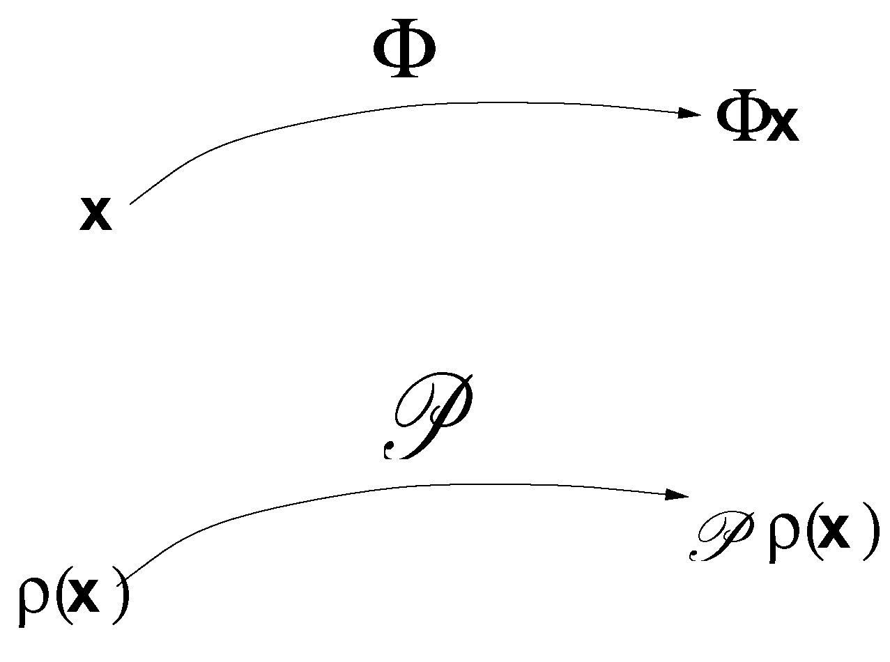
For discrete systems in the form of Equation (4), as $\mathit{x}$ is carried forth under the transformation Φ, there is another transformation, called Frobenius–Perron operator $\mathcal{P}$ (F-P operator hereafter), steering $\rho \left(\mathit{x}\right)$, i.e., the pdf of $\mathit{x}$, to $\mathcal{P}\rho$ (see a schematic in Figure 1). The F-P operator governs the evolution of the density of $\mathit{x}$.

A rigorous definition requires some ingredients of measure theory which is beyond the scope this review, and the reader may consult with the reference [50]. Loosely speaking, given a transformation $\Phi :\Omega \to \Omega$ (in this review, $\Omega ={\mathbb{R}}^n$), $\mathit{x}\mapsto \Phi \mathit{x}$, it is a mapping $\mathcal{P}:L^1\left({\Omega }^n\right)\to L^1\left({\Omega }^n\right)$, $\rho \mapsto \mathcal{P}\rho$, such that

$$\begin{array}{c}\hfill {\int }_{\omega }\mathcal{P}\rho \left(\mathit{x}\right)d\mathit{x}={\int }_{{\Phi }^{-1}\left(\omega \right)}\rho \left(\mathit{x}\right)d\mathit{x}\end{array}$$

(17)

for any $\omega \subset \Omega$. If Φ is nonsingular and invertible, it actually can be explicitly evaluated. Making transformation $\mathit{y}=\Phi \left(\mathit{x}\right)$, the right hand side is, in this case,

$$\begin{array}{c}\hfill {\int }_{{\Phi }^{-1}\left(\omega \right)}\rho \left(\mathit{x}\right)d\mathit{x}={\int }_{\omega }\rho \left[{\Phi }^{-1}\left(\mathit{y}\right)\right]·\left|J^{-1}\right|d\mathit{y}\end{array}$$

where J is the Jacobian of Φ:

$$\begin{array}{c}\hfill J=det\left[\frac{\partial (y_1,y_2,\dots y_n)}{\partial (x_1,x_2,\dots x_n)}\right]\end{array}$$

and $J^{-1}$ its inverse. Since ω is arbitrarily chosen, we have

$$\begin{array}{c}\hfill \mathcal{P}\rho \left(\mathit{x}\right)=\rho \left[{\Phi }^{-1}\left(\mathit{x}\right)\right]·\left|J^{-1}\right|\end{array}$$

(18)

If no nonsingularity is assumed for the transformation Φ, but the sample space Ω is in a Cartesian product form, as is for this review, the F-P operator can also be evaluated, though not in an explicit form. Consider a domain

$$\begin{array}{c}\hfill \omega =[a_1,x_1]\times [a_2,x_2]\times \dots \times [a_n,x_n]\end{array}$$

where $\mathit{a}=(a_1,\dots ,a_n)$ is some constant point (usually can be set to be the origin). Let the counterimage of ω be ${\Phi }^{-1}\left(\omega \right)$, then it has been proved (c.f. [50]) that

$$\begin{array}{c}\hfill \mathcal{P}\rho \left(\mathit{x}\right)=\frac{{\partial }^n}{\partial x_n\dots \partial x_2\partial x_1}{\int }_{{\Phi }^{-1}\left(\omega \right)}\rho ({\xi }_1,{\xi }_2,\dots ,{\xi }_n)d{\xi }_{1}d{\xi }_2\dots d{\xi }_n\end{array}$$

In this review, we consider a sample space ${\mathbb{R}}^n$, so essentially all the F-P operators can be calculated this way.

Figure 1. Illustration of the Frobenius-Perron operator $\mathcal{P}$, which takes $\rho \left(\mathit{x}\right)$ to $\mathcal{P}\rho \left(\mathit{x}\right)$ as Φ takes $\mathit{x}$ to $\Phi \mathit{x}$.

Figure 1. Illustration of the Frobenius-Perron operator $\mathcal{P}$, which takes $\rho \left(\mathit{x}\right)$ to $\mathcal{P}\rho \left(\mathit{x}\right)$ as Φ takes $\mathit{x}$ to $\Phi \mathit{x}$.

3.2. Information Flow

The F-P operator $\mathcal{P}$ allows for an evaluation of the change of entropy as the system evolves forth. By the formalism (16) , we need to examine how the marginal entropy changes on a time interval $[\tau ,\tau +1]$. Without loss of generality, consider only the flow from $x_2$ to $x_1$. First look at increase of $H_1$. Let ρ be the joint density at step τ, then the joint density at step $\tau +1$ is $\mathcal{P}\rho$, and hence

$$\begin{array}{ccc}\hfill \Delta H_1& =& H_1(\tau +1)-H_1\left(\tau \right)\hfill \\ & =& -{\int }_{\mathbb{R}}{\left(\mathcal{P}\rho \right)}_1\left(y_1\right)·log{\left(\mathcal{P}\rho \right)}_1\left(y_1\right)d{y}_1+{\int }_{\mathbb{R}}{\rho }_1\left(x_1\right)·log{\rho }_1\left(x_1\right)d{x}_1\hfill \end{array}$$

(19)

Here ${\left(\mathcal{P}\rho \right)}_1$ means the marginal density of $x_1$ at $\tau +1$; it is equal to $\mathcal{P}\rho$ with all components of $\mathit{x}$ but $x_1$ being integrated out. The independent variables with respect to which the integrations are taken are dummy; but for the sake of clarity, we use different notations, i.e., x and y, for them at time step τ and $\tau +1$, respectively.

The key to the formalism (16) is the finding of

$$\begin{array}{c}\hfill \Delta H_{1\setminus 2}=H_{1\setminus 2}(\tau +1)-H_1\left(\tau \right)\end{array}$$

(20)

namely the increment of the marginal entropy of $x_1$ on $[\tau ,\tau +1]$ with the contribution from $x_2$ excluded. Here the system in question is no longer Equation (4), but a system with a mapping modified from Φ:

$$\begin{array}{c}\hfill {\Phi }_{\setminus 2}:\left\{\begin{array}{cc}{y}_1=\hfill & {\Phi }_1(x_1,x_2,x_3,\dots ,x_n)\hfill \\ y_3=\hfill & {\Phi }_3(x_1,x_2,x_3,\dots ,x_n)\hfill \\ ⋮\hfill & ⋮\hfill \\ y_n=\hfill & {\Phi }_n(x_1,x_2,x_3,\dots ,x_n)\hfill \end{array}\right.\end{array}$$

(21)

with $x_2$ frozen instantaneously at τ as a parameter. Again, we use $x_i=x_i\left(\tau \right)$, $y_i=\Phi \left(\mathit{x}\left(\tau \right)\right)=x_i(\tau +1)$, $i=1,\dots ,n$, to indicate the state variables at steps τ and $\tau +1$, respectively, to avoid any possible confusion. In the mean time, the dependence on τ and $\tau +1$ are suppressed for notational economy. Corresponding to the modified transformation ${\Phi }_{\setminus 2}$ is a modified F-P operator, written ${\mathcal{P}}_{\setminus 2}$. To find $H_{1\setminus 2}(\tau +1)$, examine the quantity $h=-log{\left({\mathcal{P}}_{\setminus 2}\rho \right)}_1\left(y_1\right)$, where the subscript 1 indicates that this is a marginal density of the first component, and the dependence on $y_1$ tells that this is evaluated at step $\tau +1$. Recall how Shannon entropy is defined: $H_{1\setminus 2}(\tau +1)$ is essentially the mathematical expectation, or “average” in loose language, of h. More specifically, it is h multiplied with some pdf followed by an integration over ${\mathbb{R}}^n$, i.e., the corresponding sample space. The pdf is composed of several different factors. The first is, of course, ${\left({\mathcal{P}}_{\setminus 2}\rho \right)}_1\left(y_1\right)$. But h, as well as ${\left({\mathcal{P}}_{\setminus 2}\rho \right)}_1$, also has dependence on $x_2$, which is embedded within the subscript $\setminus 2$. Recall how $x_2$ is treated during $[\tau ,\tau +1]$: It is frozen at step τ and kept on as a parameter, given all other components at τ. Therefore, the second part of the density is $\rho \left(x_2\right|x_1,x_3,\dots ,x_n)$, i.e., the conditional density of $x_2$ on $x_1,x_3,\dots ,x_n$. (Note again that $x_i$ means variables at time step τ.) This factor introduces extra dependencies: $x_3$, $x_4$, ..., $x_n$ (that of $x_1$ is embedded in $y_1$), which must also be averaged out, so the third factor of the density is ${\rho }_{3\dots n}(x_3,\dots ,x_n)$ namely the joint density of $(x_3,x_4,\dots ,x_n)$. Put all these together,

$$\begin{array}{ccc}\hfill H_{1\setminus 2}(\tau +1)& =& -{\int }_{{\mathbb{R}}^n}{\left({\mathcal{P}}_{\setminus 2}\rho \right)}_1\left(y_1\right)·log{\left({\mathcal{P}}_{\setminus 2}\rho \right)}_1\left(y_1\right)·\rho \left(x_2\right|x_1,x_3,\dots ,x_n)\hfill \\ & & ·{\rho }_{3\dots n}(x_3,\dots ,x_n)d{y}_{1}d{x}_{2}d{x}_3\dots d{x}_n\hfill \end{array}$$

(22)

Subtraction of $H_{1\setminus 2}(\tau +1)-H_1\left(\tau \right)$ from Equation (19) gives, eventually, the rate of information flow/transfer from $x_2$ to $x_1$:

$$\begin{array}{ccc}\hfill T_{2\to 1}& =& -{\int }_{\mathbb{R}}{\left(\mathcal{P}\rho \right)}_1\left(y_1\right)·log{\left(\mathcal{P}\rho \right)}_1\left(y_1\right)d{y}_1\hfill \\ & & +{\int }_{{\mathbb{R}}^n}{\left({\mathcal{P}}_{\setminus 2}\rho \right)}_1\left(y_1\right)·log{\left({\mathcal{P}}_{\setminus 2}\rho \right)}_1\left(y_1\right)·\rho \left(x_2\right|x_1,x_3,\dots ,x_n)·\hfill \\ & & {\rho }_{3\dots n}(x_3,\dots ,x_n)d{y}_{1}d{x}_{2}d{x}_3\dots d{x}_n\hfill \end{array}$$

(23)

Notice that the conditional density of $x_2$ is on $x_1$, not on $y_1$. ($x_1$ and $y_1$ are the same state variable evaluated at different time steps, and are connected via $y_1={\Phi }_1(x_1,x_2,\dots ,x_n)$.

Likewise, it is easy to obtain the information flow between any pair of components. If, for example, we are concerned with the flow from $x_j$ to $x_i$ ($i,j=1,2,\dots ,n$, $i\ne j$), replacement of the indices 1 and 2 in Equation (23) respectively with i and j gives

$$\begin{array}{ccc}\hfill T_{j\to i}& =& -{\int }_{\mathbb{R}}{\left(\mathcal{P}\rho \right)}_i\left(y_i\right)·log{\left(\mathcal{P}\rho \right)}_i\left(y_i\right)d{y}_i\hfill \\ & & +{\int }_{{\mathbb{R}}^n}{\left({\mathcal{P}}_{\setminus j}\rho \right)}_i\left(y_i\right)·log{\left({\mathcal{P}}_{\setminus j}\rho \right)}_1\left(y_i\right)·\rho \left(x_j\right|x_1,x_2,\dots ,x_{j-1},x_{j+1},\dots ,x_n)·\hfill \\ & & {\rho }_{\setminus i\setminus j}d{x}_{1}d{x}_2\dots d{x}_{i-1}d{y}_{i}d{x}_{i+1}\dots d{x}_n\hfill \end{array}$$

(24)

Here the subscript $\setminus j$ of $\mathcal{P}$ means the F-P operator with the effect of the $j^{\mathrm{th}}$ component excluded through freezing it instantaneously as a parameter. We have also abused the notation a little bit for the density function to indicate the marginalization of that component. That is to say,

$$\begin{array}{c}\hfill {\rho }_{\setminus i}={\rho }_{\setminus i}(x_1,\dots ,x_{i-1},x_{i+1},\dots ,x_n)={\int }_{\mathbb{R}}\rho \left(\mathit{x}\right)d{x}_i\end{array}$$

(25)

and ${\rho }_{\setminus i\setminus j}$ is the density after being marginalized twice, with respect to $x_i$ and $x_j$. To avoid this potential notation complexity, alternatively, one may reorganize the order of the components of the vector $\mathit{x}={(x_1,\dots ,x_n)}^T$ such that the pair appears in the first two slots, and modify the mapping Φ accordingly. In this case, the flow/transfer is precisely the same in form as Equation (23). Equations (23) and (24) can be evaluated explicitly for systems that are definitely specified. In the following sections we will see several concrete examples.

3.3. Properties

The information flow obtained in Equations (23) or (24) has some nice properties. The first is a concretization of the transfer asymmetry emphasized by Schreiber [47] (as mentioned in the introduction), and the second a special property for 2D systems.

Theorem 3.1 

For the system Equation (4), if ${\Phi }_i$ is independent of $x_j$, then $T_{j\to i}=0$ (in the mean time, $T_{i\to j}$ need not be zero).

The proof is rather technically involved; the reader is referred to [48] for details. This theorem states that, if the evolution of $x_i$ has nothing to do with $x_j$, then there will be no information flowing from $x_j$ to $x_i$. This is in agreement with observations, and with what one would argue on physical grounds. On the other hand, the vanishing $T_{j\to i}$ yields no clue on $T_{i\to j}$, i.e., the flow from $x_i$ to $x_j$ need not be zero in the mean time, unless ${\Phi }_j$ does not rely on $x_i$. This is indicative of a very important physical fact: information flow between a component pair is not symmetric, in contrast to the notion of mutual information ever existing in information theory. As emphasized by Schreiber [47], a faithful formalism must be able to recover this asymmetry. The theorem shows that our formalism yields precisely what is expected. Since transfer asymmetry is a reflection of causality, the above theorem is also referred to as property of causality by Liang and Kleeman [48].

Theorem 3.2 

For the system Equation (4), if $n=2$ and ${\Phi }_1$ is invertible, then $T_{2\to 1}=\Delta H_1-Elog\left|J_1\right|$, where $J_1=\partial {\Phi }_1/\partial x_1$.

A brief proof will help to gain better understanding of the theorem. If $n=2$, the modified system has a mapping ${\Phi }_{\setminus 2}$ which is simply ${\Phi }_1$ with $x_2$ as a parameter. Equation (22) is thus reduced to

$$\begin{array}{ccc}\hfill H_{1\setminus 2}(\tau +1)& =& -{\int }_{{\mathbb{R}}^2}{\left({\mathcal{P}}_{\setminus 2}\rho \right)}_1\left(y_1\right)·log{\left({\mathcal{P}}_{\setminus 2}\rho \right)}_1\left(y_1\right)·\rho \left(x_2\right|x_1)d{y}_{1}d{x}_2\hfill \end{array}$$

where $y_1={\Phi }_1(x_1,x_2)$, and ${\left({\mathcal{P}}_{\setminus 2}\rho \right)}_1$ the marginal density of $x_1$ evolving from ${\rho }_{\setminus 2}={\rho }_1$ upon one transformation of ${\Phi }_{\setminus 2}={\Phi }_1$. By assumption ${\Phi }_1$ is invertible, that is to say, $J_1=\frac{\partial {\Phi }_1}{\partial x_1}\ne 0$. The F-P operator hence can be explicitly written out:

$$\begin{array}{ccc}\hfill {\left({\mathcal{P}}_{\setminus 2}\rho \right)}_1\left(y_1\right)& =& \rho \left[{\Phi }_1^{-1}(y_1,x_2)\right]·\left|J_1^{-1}\right|\hfill \\ & =& {\rho }_1\left(x_1\right)\left|J_1^{-1}\right|\hfill \end{array}$$

(26)

So

$$\begin{array}{ccc}\hfill \Delta H_{1\setminus 2}& =& H_{1\setminus 2}(\tau +1)-H_1\left(\tau \right)\hfill \\ & =& -{\int }_{{\mathbb{R}}^2}{\rho }_1\left(x_1\right)\left|J_1^{-1}\right|log\left({\rho }_1\left(x_1\right)\left|J_1^{-1}\right|\right)\rho \left(x_2\right|x_1)\left|J_1\right|d{x}_{1}d{x}_2+{\int }_{\mathbb{R}}{\rho }_{1}log{\rho }_{1}d{x}_1\hfill \\ & =& -{\int }_{{\mathbb{R}}^2}{\rho }_1\left(x_1\right)\rho \left(x_2\right|x_1)log\left|J_1^{-1}\right|d{x}_{1}d{x}_2\hfill \\ & =& {\int }_{{\mathbb{R}}^2}\rho (x_1,x_2)log\left|J_1\right|d{x}_{1}d{x}_2\hfill \\ & =& Elog\left|J_1\right|\hfill \end{array}$$

(27)

The conclusion follows subsequently from Equation (16).

The above theorem actually states another interesting fact that parallels what we introduced previously in §2.2 via heuristic reasoning. To see this, reconsider the mapping $\Phi :{\mathbb{R}}^n\to {\mathbb{R}}^n$, $\mathit{x}\mapsto \mathit{x}$. Let Φ be nonsingular and invertible. By Equation (18), the F-P operator of the joint pdf ρ can be explicitly evaluated. Accordingly, the entropy increases, as time moves from step τ to step $\tau +1$, by

$$\begin{array}{ccc}\hfill \Delta H& =& -{\int }_{{\mathbb{R}}^n}\mathcal{P}\rho \left(\mathit{x}\right)log\mathcal{P}\rho \left(\mathit{x}\right)d\mathit{x}+{\int }_{{\mathbb{R}}^n}\rho \left(\mathit{x}\right)log\rho \left(\mathit{x}\right)d\mathit{x}\hfill \\ & =& -{\int }_{{\mathbb{R}}^n}\rho \left[{\Phi }^{-1}\left(\mathit{x}\right)\right]\left|J^{-1}\right|log\rho \left[{\Phi }^{-1}\left(\mathit{x}\right)\right]\left|J^{-1}\right|d\mathit{x}+{\int }_{{\mathbb{R}}^n}\rho \left(\mathit{x}\right)log\rho \left(\mathit{x}\right)d\mathit{x}\hfill \end{array}$$

After some manipulation (see [48] for details), this is reduced to

$$\begin{array}{c}\hfill \Delta H=Elog\left|J\right|\end{array}$$

(28)

This is the discrete counterpart of Equation (12), yet another remarkably concise formula. Now, if the system in question is 2-dimensional, then, as argued in §2.2, the information flow from $x_2$ to $x_1$ should be $\Delta H_1-\Delta H_1^{*}$, with $\Delta H_1^{*}$ being the marginal entropy increase due to $x_1$ itself. Furthermore, if ${\Phi }_1$ is nonsingular and invertible, then Equation (28) tells us it must be that

$$\begin{array}{c}\hfill \Delta H_1^{*}=Elog\left|J_1\right|\end{array}$$

and this is precisely what Theorem 3.2 reads.

4. Continuous Systems

For continuous systems in the form of Equation (3), we may take advantage of what we already have from the previous section to obtain the information flow. Without loss of generality, consider only the flow/transfer from $x_2$ to $x_1$, $T_{2\to 1}$. We adopt the following strategy to fulfill the task:

• Discretize the continuous system in time on $[t,t+\Delta t]$, and construct a mapping Φ to take $\mathit{x}\left(t\right)$ to $\mathit{x}(t+\Delta t)$;
• Freeze $x_2$ in Φ throughout $[t,t+\Delta t]$ to obtain a modified mapping ${\Phi }_{\setminus 2}$;
• Compute the marginal entropy change $\Delta H_1$ as Φ steers the system from t to $t+\Delta t$;
• Derive the marginal entropy change $\Delta H_{1\setminus 2}$ as ${\Phi }_{\setminus 2}$ steers the modified system from t to $t+\Delta t$;
• Take the limit

  $$T_{2\to 1}=\underset{\Delta t\to 0}{lim}\frac{\Delta H_1-\Delta H_{1\setminus 2}}{\Delta t}$$

  to arrive at the desiderata.

4.1. Discretization of the Continuous System

As the first step, construct out of Equation (3) an n-dimensional discrete system, which steers $\mathit{x}\left(t\right)=(x_1,x_2,\dots ,x_n)$ to $\mathit{x}(t+\Delta t)$. To avoid any confusion that may arise, $\mathit{x}(t+\Delta t)$ will be denoted as $\mathit{y}=(y_1,y_2,\dots ,y_n)$ hereafter. Discretization of Equation (3) results in a mapping, to the first order of $\Delta t$, $\Phi =({\Phi }_1,{\Phi }_2,\dots ,{\Phi }_n)$: ${\mathbb{R}}^n\to {\mathbb{R}}^n$, $\mathit{x}\mapsto \mathit{y}$:

$$\begin{array}{c}\hfill \Phi :\left\{\begin{array}{cc}{y}_1=\hfill & x_1+\Delta t·F_1\left(\mathit{x}\right)\hfill \\ y_2=\hfill & x_2+\Delta t·F_2\left(\mathit{x}\right)\hfill \\ ⋮\hfill & ⋮\hfill \\ y_n=\hfill & x_n+\Delta t·F_n\left(\mathit{x}\right)\hfill \end{array}\right.\end{array}$$

(29)

Clearly, this mapping is always invertible so long as $\Delta t$ is small enough. In fact, we have

$$\begin{array}{c}\hfill {\Phi }^{-1}:\left\{\begin{array}{cc}{x}_1=\hfill & y_1-\Delta t·F_1\left(\mathit{y}\right)+O(\Delta t^2)\hfill \\ x_2=\hfill & y_2-\Delta t·F_2\left(\mathit{y}\right)+O(\Delta t^2)\hfill \\ ⋮\hfill & ⋮\hfill \\ x_n=\hfill & y_n-\Delta t·F_n\left(\mathit{y}\right)+O(\Delta t^2)\hfill \end{array}\right.\end{array}$$

(30)

to the first order of $\Delta t$. Furthermore, its Jacobian J is

$$\begin{array}{ccc}\hfill J& =& det\left[\frac{\partial (y_1,y_2,\dots y_n)}{\partial (x_1,x_2,\dots x_n)}\right]\hfill \\ & =& \prod _i\left(1+\Delta t\frac{\partial F_i}{\partial x_i}\right)+O(\Delta t^2)\hfill \\ & =& 1+\Delta t\sum _{i=1}^n\frac{\partial F_i}{\partial x_i}+O(\Delta t^2)\hfill \end{array}$$

(31)

Likewise, it is easy to get

$$\begin{array}{ccc}\hfill J^{-1}=& =& det\left[\frac{\partial (x_1,x_2,\dots x_n)}{\partial (y_1,y_2,\dots y_n)}\right]\hfill \\ & =& 1-\Delta t\sum _{i=1}^n\frac{\partial F_i}{\partial x_i}+O(\Delta t^2)\hfill \end{array}$$

(32)

This makes it possible to evaluate the F-P operator associated with Φ. By Equation (18),

$$\begin{array}{ccc}\hfill \mathcal{P}\rho (y_1,\dots ,y_n)& =& \rho \left({\Phi }^{-1}(y_1,\dots y_n)\right)\left|J^{-1}\right|\hfill \\ & =& \rho (x_1,x_2,\dots ,x_n)·\left|1-\Delta t\nabla ·\mathit{F}\right|+O(\Delta t^2)\hfill \end{array}$$

(33)

Here $\nabla ·\mathit{F}={\sum }_i\frac{\partial F_i}{\partial x_1}$; we have suppressed its dependence on $\mathit{x}$ to simplify the notation.

As an aside, the explicit evaluation (31), and subsequently (32) and (33), actually can be utilized to arrive at the important entropy evolution law (12) without invoking any assumptions. To see this, recall $\Delta H=Elog\left|J\right|$ by Equation (28). Let $\Delta t$ go to zero to get

$$\begin{array}{ccc}\hfill \frac{dH}{dt}& =& \underset{\Delta t\to 0}{lim}\frac{\Delta H}{\Delta t}=E\underset{\Delta t\to 0}{lim}\frac{1}{\Delta t}log\left(1+\Delta t\nabla ·\mathit{F}+O(\Delta t^2)\right)\hfill \end{array}$$

which is the very result $E(\nabla ·\mathit{F})$, just as one may expect.

4.2. Information Flow

To compute the information flow $T_{2\to 1}$, we need to know $d{H}_1/dt$ and $d{H}_{1\setminus 2}/dt$. The former is easy to find from the Liouville equation associated with Equation (3), i.e.,

$$\begin{array}{c}\hfill \frac{\partial \rho }{\partial t}+\frac{\partial \left(F_1\rho \right)}{\partial x_1}+\frac{\partial \left(F_2\rho \right)}{\partial x_2}+\dots +\frac{\partial \left(F_n\rho \right)}{\partial x_n}=0\end{array}$$

(34)

following the same derivation as that in §2.2:

$$\begin{array}{c}\hfill \frac{d{H}_1}{dt}={\int }_{{\mathbb{R}}^n}log{\rho }_1\frac{\partial \left(F_1\rho \right)}{\partial x_1}d\mathit{x}\end{array}$$

(35)

The challenge lies in the evaluation of $d{H}_{1\setminus 2}/dt$. We summarize the result in the following proposition:

Proposition 4.1 

For the dynamical system (3), the rate of change of the marginal entropy of $x_1$ with the effect of $x_2$ instantaneously excluded is:

$$\begin{array}{ccc}\hfill \frac{d{H}_{1\setminus 2}}{dt}& =& {\int }_{{\mathbb{R}}^n}(1+log{\rho }_1)·\frac{\partial \left(F_1{\rho }_{\setminus 2}\right)}{\partial x_1}·{\Theta }_{2|1}d\mathit{x}+\hfill \\ & & {\int }_{{\mathbb{R}}^n}{\rho }_{1}log{\rho }_1·F_1·\frac{\partial (\rho /{\rho }_{\setminus 2})}{\partial x_1}·{\rho }_{\setminus 1\setminus 2}d\mathit{x}\hfill \end{array}$$

(36)

where

$$\begin{array}{ccc}& & {\theta }_{2|1}={\theta }_{2|1}(x_1,x_2,x_3,\dots ,x_n)=\frac{\rho }{{\rho }_{\setminus 2}}{\rho }_{\setminus 1\setminus 2}\hfill \end{array}$$

(37)

$$\begin{array}{ccc}& & {\Theta }_{2|1}={\int }_{{\Omega }_{{\mathbb{R}}^{n-2}}}{\theta }_{2|1}\left(\mathit{x}\right)d{x}_3\dots d{x}_n\hfill \end{array}$$

(38)

and ${\rho }_{\setminus 2}={\int }_{\mathbb{R}}\rho d{x}_2$, ${\rho }_{\setminus 1\setminus 2}={\int }_{{\mathbb{R}}^2}\rho d{x}_{1}d{x}_2$ are the densities after marginalized with $x_2$ and $(x_1,x_2)$, respectively.

The proof is rather technically involved; for details, see [51], section 5.

With the above result, subtract $d{H}_{1\setminus 2}/dt$ from $d{H}_1/dt$ and one obtains the flow rate from $x_2$ to $x_1$. Likewise, the information flow between any component pair $(x_i,x_j)$, $i,j=1,2,\dots ,n$; $i\ne j$, can be obtained henceforth.

Theorem 4.1 

For the dynamical system Equation (3), the rate of information flow from $x_j$ to $x_i$ is

$$\begin{array}{ccc}\hfill T_{j\to i}& =& {\int }_{\Omega }(1+log{\rho }_i)\left(\frac{\partial \left(F_i\rho \right)}{\partial x_i}-\frac{\partial \left(F_i{\rho }_{\setminus j}\right)}{\partial x_i}·{\Theta }_{j|i}\right)d\mathit{x}\hfill \\ & +& {\int }_{\Omega }\frac{\partial (F_i{\rho }_{i}log{\rho }_i)}{\partial x_i}·{\theta }_{j|i}d\mathit{x}\hfill \end{array}$$

(39)

where

$$\begin{array}{ccc}& & {\theta }_{j|i}={\theta }_{j|i}\left(\mathit{x}\right)=\frac{\rho }{{\rho }_{\setminus j}}{\rho }_{\setminus i\setminus j}\hfill \end{array}$$

(40)

$$\begin{array}{ccc}& & {\rho }_{\setminus i}={\int }_{\mathbb{R}}\rho \left(\mathit{x}\right)d{x}_i\hfill \end{array}$$

(41)

$$\begin{array}{ccc}& & {\rho }_{\setminus i\setminus j}={\int }_{{\mathbb{R}}^2}\rho \left(\mathit{x}\right)d{x}_{i}d{x}_j\hfill \end{array}$$

(42)

$$\begin{array}{ccc}& & {\Theta }_{j|i}={\Theta }_{j|i}(x_i,x_j)={\int }_{{\mathbb{R}}^{n-2}}{\theta }_{j|i}\left(\mathit{x}\right)\prod _{\nu \ne i,j}d{x}_{\nu }\hfill \end{array}$$

(43)

In this formula, ${\Theta }_{j|i}$ reminds one of the conditional density $x_j$ on $x_i$, and, if $n=2$, it is indeed so. We may therefore call it the “generalized conditional density” of $x_j$ on $x_i$.

4.3. Properties

Recall that, as we argue in §2.2 based on the entropy evolution law (12), the time rate of change of the marginal entropy of a component, say $x_1$, due to its own reason, is $d{H}_1^{*}/dt=E(\partial F_1/\partial x_1)$. Since for a 2D system, $d{H}_1^{*}/dt$ is precisely $d{H}_{1\setminus 2}/dt$, we expect that the above formalism (36) or (39) verifies this result.

Theorem 4.2 

If the system Equation (3) has a dimensionality 2, then

$$\begin{array}{c}\hfill \frac{d{H}_{1\setminus 2}}{dt}=E\left(\frac{\partial F_1}{\partial x_1}\right)\end{array}$$

(44)

and hence the rate of information flow from $x_2$ to $x_1$ is

$$\begin{array}{c}\hfill T_{2\to 1}=-E\left[\frac{1}{{\rho }_1}\frac{\partial \left(F_1{\rho }_1\right)}{\partial x_1}\right]\end{array}$$

(45)

What makes a 2D system so special is that, when $n=2$, ${\rho }_{\setminus 2}={\rho }_1$, and ${\Theta }_{2|1}$ is just the conditional distribution of $x_2$ given $x_1$, $\rho /{\rho }_1=\rho \left(x_2\right|x_1)$. Equation (36) can thereby be greatly simplified:

$$\begin{array}{ccc}\hfill \frac{d{H}_{1\setminus 2}}{dt}& =& {\int }_{{\mathbb{R}}^n}(1+log{\rho }_1)\frac{\partial F_1{\rho }_1}{\partial x_1}·\frac{\rho }{{\rho }_1}d\mathit{x}+{\int }_{{\mathbb{R}}^n}{\rho }_{1}log{\rho }_1·F_1·\frac{\partial \rho \left(x_2\right|x_1)}{\partial x_1}d\mathit{x}\hfill \\ & =& {\int }_{{\mathbb{R}}^n}\frac{\partial \left(F_1{\rho }_1\right)}{\partial x_1}\frac{\rho }{{\rho }_1}d\mathit{x}+{\int }_{{\mathbb{R}}^n}log{\rho }_1·\frac{\partial \left(F_1\rho \right)}{\partial x_1}d\mathit{x}\hfill \\ & =& {\int }_{{\mathbb{R}}^n}\rho \left(\frac{\partial F_1}{\partial x_1}\right)d\mathit{x}=E\left(\frac{\partial F_1}{\partial x_1}\right)\hfill \end{array}$$

(46)

Subtract this from what has been obtained above for $d{H}_1/dt$, and we get an information flow just as that in Equation (14) via heuristic argument.

As in the discrete case, one important property that $T_{j\to i}$ must possess is transfer asymmetry, which has been emphasized previously, particularly by Schreiber [47]. The following is a concretization of the argument.

Theorem 4.3 (Causality) 

For system (3), if $F_i$ is independent of $x_j$, then $T_{j\to i}=0$; in the mean time, $T_{i\to j}$ need not vanish, unless $F_j$ has no dependence on $x_i$.

Look at the right-hand side of the formula (39). Given that $(1+log{\rho }_i)$ and ${\rho }_{\setminus j}$, as well as $F_i$ (by assumption), are independent of $x_j$, the integration with respect to $x_j$ can be taken within the multiple integrals. Consider the second integral first. All the variables except ${\theta }_{j|i}$ have dependence on $x_j$. But $\int {\theta }_{j|i}d{x}_j=1$, so the whole term is equal to ${\int }_{{\mathbb{R}}^{n-1}}\frac{\partial (F_i{\rho }_{i}log{\rho }_i)}{\partial x_i}d{x}_1\dots d{x}_{j-1}d{x}_{j+1}\dots d{x}_n$ which vanishes by the assumption of compact support. For the first integral, move the integration with respect to $x_j$ into the parentheses, as the factor outside has nothing to do with $x_j$. This integration yields

$$\begin{array}{ccc}& & {\int }_{\mathbb{R}}\frac{\partial \left(F_i\rho \right)}{\partial x_i}d{x}_j-{\int }_{\mathbb{R}}\frac{\partial \left(F_i{\rho }_{\setminus j}\right)}{\partial x_i}·{\Theta }_{j|i}d{x}_j\hfill \\ & & ={\int }_{{\mathbb{R}}^{n-1}}\left[\frac{\partial }{\partial x_i}\left(F_i\int \rho d{x}_j\right)-\frac{\partial }{\partial x_i}\left(F_i{\rho }_{\setminus j}\right)·\int {\Theta }_{j|i}d{x}_j\right]d{x}_1\dots d{x}_{j-1}d{x}_{j+1}\dots d{x}_n\hfill \\ & & =0\hfill \end{array}$$

because $\int \rho d{x}_j={\rho }_{\setminus j}$ and $\int {\Theta }_{j|i}d{x}_j=1$. For all that account, both the two integrals on the right-hand side of Equation (39) vanish, leaving a zero flow of information from $x_j$ to $x_i$. Notice that this vanishing $T_{j\to i}$ gives no hint on the flow in the opposite direction. In other words, this kind of flow or transfer is not symmetric, reflecting the causal relation between the component pair. As Theorem 3.1 is for discrete systems, Theorem 4.3 is the property of causality for continuous systems.

5. Stochastic Systems

So far, all the systems considered are deterministic. In this section we turn to systems with stochasticity included. Consider the stochastic counterpart of Equation (3)

$$\begin{array}{c}\hfill d\mathit{x}=\mathit{F}(\mathit{x},t)dt+\mathit{B}(\mathit{x},t)d\mathit{w}\end{array}$$

(47)

where $\mathit{w}$ is a vector of standard Wiener processes, and $\mathit{B}=\left(b_{ij}\right)$ the matrix of perturbation amplitudes. In this section, we limit our discussion to 2D systems, and hence have only two flows/transfers to discuss. Without loss of generality, consider only $T_{2\to 1}$, i.e., the rate of flow/transfer from $x_2$ to $x_1$.

As before, we first need to find the time rate of change of $H_1$, the marginal entropy of $x_1$. This can be easily derived from the density evolution equation corresponding to Equation (47), i.e., the Fokker-Planck equation:

$$\begin{array}{c}\hfill \frac{\partial \rho }{\partial t}+\frac{\partial \left(F_1\rho \right)}{\partial x_1}+\frac{\partial \left(F_2\rho \right)}{\partial x_2}=\frac{1}{2}\sum _{i,j=1}^2\frac{{\partial }^2\left(g_{ij}\rho \right)}{\partial x_i\partial x_j}\end{array}$$

(48)

where $g_{ij}=g_{ji}={\sum }_{k=1}^2{b}_{ik}{b}_{jk},$ $i,j=1,2$. This integrated over $\mathbb{R}$ with respect to $x_2$ gives the evolution of ${\rho }_1$:

$$\begin{array}{c}\hfill \frac{\partial {\rho }_1}{\partial t}+{\int }_{\mathbb{R}}\frac{\partial \left(F_1\rho \right)}{\partial x_1}d{x}_2=\frac{1}{2}{\int }_{\mathbb{R}}\frac{{\partial }^2\left(g_{11}\rho \right)}{\partial x_1^2}d{x}_2\end{array}$$

(49)

Multiply (49) by $-(1+log{\rho }_1)$, and integrate with respect to $x_1$ over $\mathbb{R}$. After some manipulation, one obtains, using the compact support assumption,

$$\begin{array}{c}\hfill \frac{d{H}_1}{dt}=-E\left(F_1\frac{\partial log{\rho }_1}{\partial x_1}\right)-\frac{1}{2}E\left(g_{11}\frac{{\partial }^{2}log{\rho }_1}{\partial x_1^2}\right)\end{array}$$

(50)

where E is the mathematical expectation with respect to ρ.

Again, the key to the formalism is the finding of $d{H}_{1\setminus 2}/dt$. For stochastic systems, this could be a challenging task. The major challenge is that we cannot obtain an F-P operator as nice as that in the previous section for the map resulting from discretization. In early days, Majda and Harlim [53] have tried our heuristic argument in §2.2 to consider a special system modeling the atmosphere–ocean interaction, which is in the form

$$\begin{array}{ccc}& & d{x}_1=F_1(x_1,x_2)dt\hfill \\ & & d{x}_2=F_2(x_1,x_2)dt+b_{22}d{w}_2\hfill \end{array}$$

Their purpose is to find $T_{2\to 1}$ namely the information transfer from $x_2$ to $x_1$. In this case, since the governing equation for $x_1$ is deterministic, the result is precisely the same as that of LK05, which is shown in in §2.2. The problem here is that the approach cannot be extended even to finding $T_{1\to 2}$, since the nice law on which the argument is based, i.e., Equation (12), does not hold for stochastic processes.

Liang (2008) [54] adopted a different approach to give this problem a solution. As in the previous section, the general strategy is also to discretize the system in time, modify the discretized system with $x_2$ frozen as a parameter on an interval $[t,t+\Delta t]$, and then let $\Delta t$ go to zero and take the limit. But this time no operator analogous to the F-P operator is sought; instead, we discretize the Fokker–Planck equation and expand $x_{1\setminus 2(t+\Delta t)}$, namely the first component at $t+\Delta t$ with $x_2$ frozen at t, using the Euler–Bernstein approximation. The complete derivation is beyond the scope of this review; the reader is referred to [54] for details. In the following, the final result is supplied in the form of a proposition.

Proposition 5.1 

For the 2D stochastic system (47), the time change of the marginal entropy of $x_1$ with the contribution from $x_2$ excluded is

$$\begin{array}{ccc}\hfill \frac{d{H}_{1\setminus 2}}{dt}& =& E\left(\frac{\partial F_1}{\partial x_1}\right)-\frac{1}{2}E\left(g_{11}\frac{{\partial }^{2}log{\rho }_1}{\partial x_1^2}\right)-\frac{1}{2}E\left(\frac{1}{{\rho }_1}\frac{{\partial }^2\left(g_{11}{\rho }_1\right)}{\partial x_1^2}\right)\hfill \end{array}$$

(51)

In the equation, the second and the third terms on the right hand side are from the stochastic perturbation. The first term, as one may recall, is precisely the result of Theorem 4.2. The heuristic argument for 2D systems in Equation (13) is successfully recovered here. With this the rate of information flow can be easily obtained by subtracting $d{H}_{1\setminus 2}/dt$ from $d{H}_1/dt$.

Theorem 5.1 

For the 2D stochastic system (47), the rate of information flow from $x_2$ to $x_1$ is

$$\begin{array}{c}\hfill T_{2\to 1}=-E\left(\frac{1}{{\rho }_1}\frac{\partial \left(F_1{\rho }_1\right)}{\partial x_1}\right)+\frac{1}{2}E\left(\frac{1}{{\rho }_1}\frac{{\partial }^2\left(g_{11}{\rho }_1\right)}{\partial x_1^2}\right)\end{array}$$

(52)

where E is the expectation with respect to $\rho (x_1,x_2)$.

It has been a routine to check for the obtained flow the property of causality or asymmetry. Here in Equation (52), the first term on the right hand side is from the deterministic part of the system, which has been checked before. For the second term, if $b_{11}$, $b_{12}$, and hence $g_{11}={\sum }_k{b}_{1k}{b}_{1k}$ have no dependence on $x_2$, then the integration with respect to $x_2$ can be taken inside with $\rho /{\rho }_1$ or $\rho \left(x_2\right|x_1)$, and results in 1. The remaining part is in a divergence form, which, by the assumption of compact support, gives a zero contribution from the stochastic perturbation. We therefore have the following theorem:

Theorem 5.2 

If, in the stochastic system (47), the evolution of $x_1$ is independent of $x_2$, then $T_{2\to 1}=0$.

The above argument actually has more implications. Suppose $\mathit{B}=\left(b_{ij}\right)$ are independent of $\mathit{x}$, i.e., the noises are uncorrelated with the state variables. This model is indeed of interest, as in the real world, a large portion of noises are additive; in other words, $b_{ij}$, and hence $g_{ij}$, are constant more often than not. In this case, no matter what the vector field $\mathit{F}$ is, by the above argument the resulting information flows within the system will involve no contribution from the stochastic perturbation. That is to say,

Theorem 5.3 

Within a stochastic system, if the noise is additive, then the information flows are the same in form as that of the corresponding deterministic system.

This theorem shows that, if only information flows are considered, a stochastic system with additive noise functions just like deterministic. Of course, the resemblance is limited to the form of formula; the marginal density ${\rho }_1$ in Equation (52) already takes into account the effect of stochasticity, as can be seen from the integrated Fokker–Planck Equation (49). A more appropriate statement might be that, for this case, stochasticity is disguised within the formula of information flow.

6. Applications

Since its establishment, the formalism of information flow has been applied with a variety of dynamical system problems. In the following we give a brief description of these applications.

6.1. Baker Transformation

The baker transformation as a prototype of an area-conserving chaotic map is one of the most studied discrete dynamical systems. Topologically it is conjugate to another well-studied system, the horseshoe map, and has been be used to model the diffusion process in real physical world.

The baker transformation mimicks the kneading of dough: first the dough is compressed, then cut in half; the two halves are stacked on one another, compressed, and so forth. Formally, it is defined as a mapping on the unit square $\Omega =[0,1]\times [0,1]$, $\Phi :\Omega \to \Omega$,

$$\begin{array}{c}\hfill \Phi (x_1,x_2)=\left\{\begin{array}{cc}(2x_1,\frac{x_2}{2}),\hfill & 0\le x_1\le \frac{1}{2},0\le x_2\le 1\hfill \\ (2x_1-1,\frac{1}{2}{x}_2+\frac{1}{2}),\hfill & \frac{1}{2}<x_1\le 1,0\le x_2\le 1\hfill \end{array}\right.\end{array}$$

(53)

with a Jacobian $J=det\left[\frac{\partial ({\Phi }_1\left(\mathit{x}\right),{\Phi }_2\left(\mathit{x}\right))}{\partial (x_1,x_2)}\right]=1$. This is the area-conserving property, which, by Equation (28) yields $\Delta H=Elog\left|J\right|=0$; that is to say, the entropy is also conserved. The nonvanishing Jacobian implies that it is invertible; in fact, it has an inverse

$$\begin{array}{c}\hfill {\Phi }^{-1}(x_1,x_2)=\left\{\begin{array}{cc}(\frac{x_1}{2},2x_2),\hfill & 0\le x_2\le \frac{1}{2},0\le x_1\le 1\hfill \\ (\frac{x_1+1}{2},2x_2-1),\hfill & \frac{1}{2}\le x_2\le 1,0\le x_1\le 1\hfill \end{array}\right.\end{array}$$

(54)

Thus the F-P operator $\mathcal{P}$ can be easily found

$$\begin{array}{c}\hfill \mathcal{P}\rho (x_1,x_2)=\rho \left[{\Phi }^{-1}(x_1,x_2)\right]·\left|J^{-1}\right|=\left\{\begin{array}{cc}\rho (\frac{x_1}{2},2x_2),\hfill & 0\le x_2<\frac{1}{2}\hfill \\ \rho (\frac{1+x_1}{2},2x_2-1),\hfill & \frac{1}{2}\le x_2\le 1\hfill \end{array}\right.\end{array}$$

(55)

First compute $T_{2\to 1}$, the information flow from $x_2$ to $x_1$. Let ${\rho }_1$ be the marginal density of $x_1$ at time step τ. Taking integration of Equation (55) with respect to $x_2$, one obtains the marginal density of $x_1$ at $\tau +1$

$$\begin{array}{ccc}\hfill {\left(\mathcal{P}\rho \right)}_1\left(x_1\right)& =& {\int }_0^{1/2}\rho (\frac{x_1}{2},2x_2)d{x}_2+{\int }_{1/2}^1\rho (\frac{x_1+1}{2},2x_2-1)d{x}_2\hfill \\ & =& \frac{1}{2}{\int }_0^1\left[\rho \left(\frac{x_1}{2},x_2\right)+\rho \left(\frac{x_1+1}{2},x_2\right)\right]d{x}_2\hfill \\ & =& \frac{1}{2}\left[{\rho }_1\left(\frac{x_1}{2}\right)+{\rho }_1\left(\frac{x_1+1}{2}\right)\right]\hfill \end{array}$$

(56)

One may also compute the marginal entropy $H_1(\tau +1)$, which is an entropy functional of ${\left(\mathcal{P}\rho \right)}_1$. However, here it is not necessary, as will soon become clear.

If, on the other hand, $x_2$ is frozen as a parameter, the transformation (53) then reduces to a dyadic mapping in the stretching direction, ${\Phi }_1:[0,1]\to [0,1]$, ${\Phi }_1\left(x_1\right)=2x_1\left(\mathrm{mod}1\right)$. For any $0<x_1<1$, The counterimage of $[0,x_1]$ is

$$\begin{array}{c}\hfill {\Phi }^{-1}\left([0,x_1]\right)=\left[0,\frac{x_1}{2}\right]\cup \left[\frac{1}{2},\frac{1+x_1}{2}\right]\end{array}$$

so

$$\begin{array}{ccc}\hfill {\left({\mathcal{P}}_{\setminus 2}\rho \right)}_1\left(x_1\right)& =& \frac{\partial }{\partial x_1}{\int }_{{\Phi }^{-1}\left([0,x_1]\right)}\rho \left(s\right)ds\hfill \\ & =& \frac{\partial }{\partial x_1}{\int }_0^{x_1/2}\rho \left(s\right)ds+\frac{\partial }{\partial x_1}{\int }_{1/2}^{(1+x_1)/2}\rho \left(s\right)ds\hfill \\ & =& \frac{1}{2}\left[\rho \left(\frac{x_1}{2}\right)+\rho \left(\frac{1+x_1}{2}\right)\right]\hfill \end{array}$$

Two observations: (1) This result is exactly the same as Equation (56), i.e., ${\left({\mathcal{P}}_{\setminus 2}\rho \right)}_1$ is equal to ${\left(\mathcal{P}\rho \right)}_1$. (2) The resulting ${\left({\mathcal{P}}_{\setminus 2}\rho \right)}_1$ has no dependence on the parameter $x_2$. The latter helps to simplify the computation of $H_{1\setminus 2}(\tau +1)$ in Equation (22): Now the integration with respect to $x_2$ can be taken inside, giving $\int \rho \left(x_2\right|x_1)d{x}_2=1$. So $H_{1\setminus 2}(\tau +1)$ is precisely the entropy functional of ${\left({\mathcal{P}}_{\setminus 2}\rho \right)}_1$. But ${\left({\mathcal{P}}_{\setminus 2}\rho \right)}_1={\left(\mathcal{P}\rho \right)}_1$ by observation (1). Thus $H_1(\tau +1)=H_{1\setminus 2}(\tau +1)$, leading to a flow/transfer

$$\begin{array}{c}\hfill T_{2\to 1}=0\end{array}$$

(57)

The information flow in the opposite direction is different. As above, first compute the marginal density

$$\begin{array}{c}\hfill {\left(\mathcal{P}\rho \right)}_2\left(x_2\right)={\int }_0^1\mathcal{P}\rho (x_1,x_2)d{x}_1=\left\{\begin{array}{cc}{\int }_0^1\rho \left(\frac{x_1}{2},2x_2\right)d{x}_1,\hfill & 0\le x_2<\frac{1}{2}\hfill \\ {\int }_0^1\rho \left(\frac{x_1+1}{2},2x_2-1\right)d{x}_1,\hfill & \frac{1}{2}\le x_2\le 1\hfill \end{array}\right.\end{array}$$

(58)

The marginal entropy increase of $x_2$ is then

$$\begin{array}{ccc}\hfill \Delta H_2& =& -{\int }_0^1{\int }_0^1\mathcal{P}\rho (x_1,x_2)·\left[log\left({\int }_0^1\mathcal{P}\rho (\lambda ,x_2)d\lambda \right)\right]d{x}_{1}d{x}_2\hfill \end{array}$$

$$\begin{array}{ccc}& & +{\int }_0^1{\int }_0^1\rho (x_1,x_2)·\left[log\left({\int }_0^1\rho (\lambda ,x_2)d\lambda \right)\right]d{x}_{1}d{x}_2,\hfill \end{array}$$

(59)

which is reduced to, after some algebraic manipulation,

$$\begin{array}{c}\hfill \Delta H_2=-log2+(I+II)\end{array}$$

(60)

where

$$\begin{array}{ccc}\hfill I& =& {\int }_0^1{\int }_0^{1/2}\rho (x_1,x_2)·\left[log\frac{{\int }_0^1\rho (\lambda ,x_2)d\lambda }{{\int }_0^{1/2}\rho (\lambda ,x_2)d\lambda }\right]d{x}_{1}d{x}_2\hfill \end{array}$$

(61)

$$\begin{array}{ccc}\hfill II& =& {\int }_0^1{\int }_{1/2}^1\rho (x_1,x_2)·\left[log\frac{{\int }_0^1\rho (\lambda ,x_2)d\lambda }{{\int }_{1/2}^1\rho (\lambda ,x_2)d\lambda }\right]d{x}_{1}d{x}_2\hfill \end{array}$$

(62)

To compute $H_{2\setminus 1}$, freeze $x_1$. The transformation is invertible and the Jacobian $J_2$ is equal to a constant $\frac{1}{2}$. By Theorem 3.2,

$$\begin{array}{c}\hfill \Delta H_{2\setminus 1}=Elog\frac{1}{2}=-log2\end{array}$$

(63)

So,

$$\begin{array}{c}\hfill T_{1\to 2}=\Delta H_2-\Delta H_{2\setminus 1}=I+II\end{array}$$

(64)

In the expressions for I and $II$, since both ρ and the terms within the brackets are nonnegative, $I+II\ge 0$. Furthermore, the two brackets cannot vanish simultaneously, hence $I+II>0$. By Equation (64) $T_{1\to 2}$ is strictly positive; in other words, there is always information flowing from $x_1$ to $x_2$.

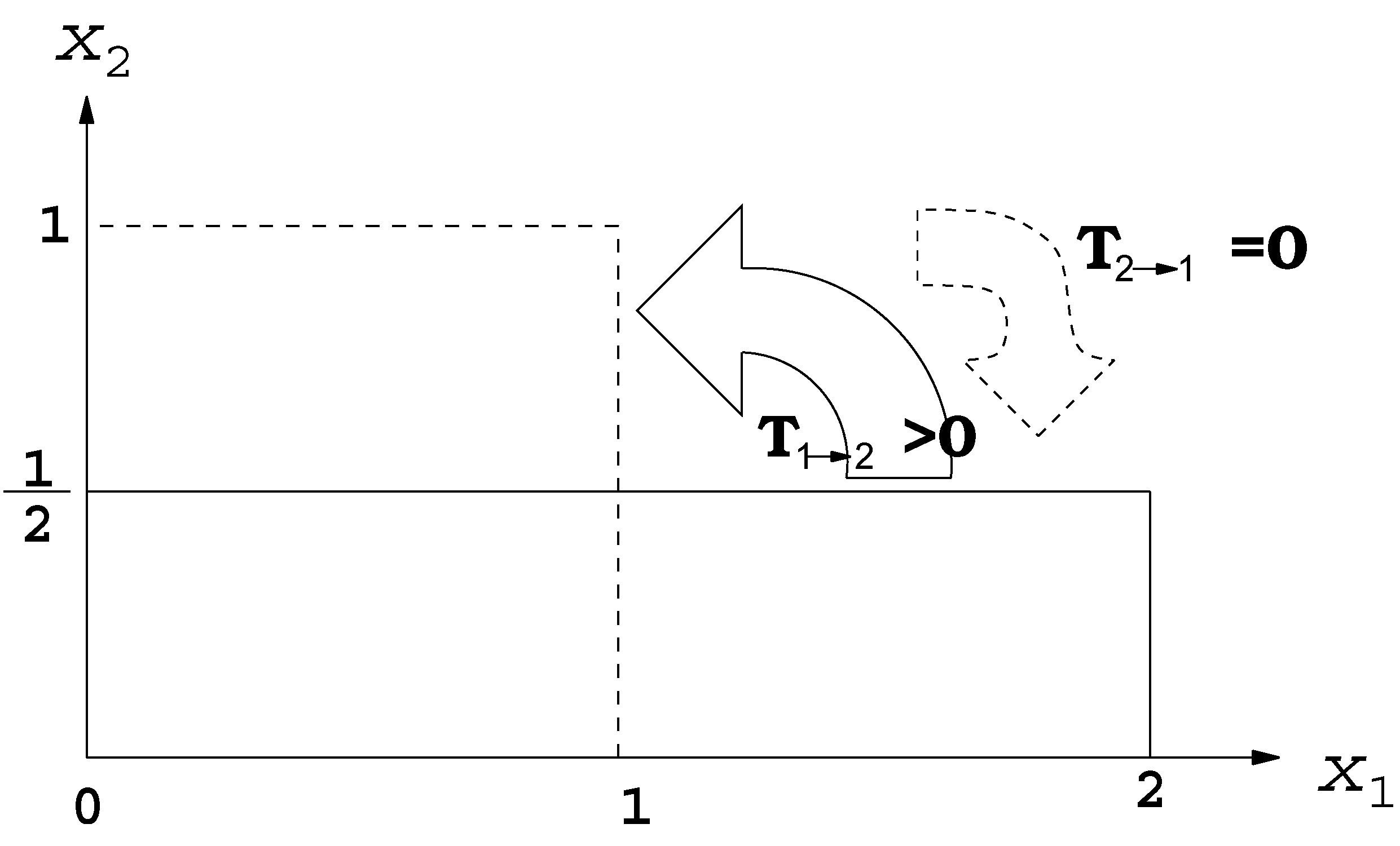
To summarize, the baker transformation transfers information asymmetrically between the two directions $x_1$ and $x_2$. As the baker stretches the dough, and folds back on top the other, information flows continuously from the stretching direction $x_1$ to the folding direction $x_2$ ($T_{1\to 2}>0$), while no transfer occurs in the opposite direction ($T_{2\to 1}=0$). These results are schematically illustrated in Figure 2; they are in agreement with what one would observe in daily life, as described in the beginning of this review.

Figure 2. Illustration of the unidirectional information flow within the baker transformation.

Figure 2. Illustration of the unidirectional information flow within the baker transformation.

6.2. H$\acute{\mathrm{e}}$non Map

The H$\acute{\mathrm{e}}$non map is another most studied discrete dynamical systems that exhibit chaotic behavior. Introduced by Michel H$\acute{\mathrm{e}}$non as a simplified Poincaré section of the Lorenz system, it is a mapping $\Phi =({\Phi }_1,{\Phi }_2):{\mathbb{R}}^2\mapsto {\mathbb{R}}^2$ defined such that

$$\begin{array}{c}\hfill \left\{\begin{array}{c}{\Phi }_1(x_1,x_2)=1+x_2-a{x}_1^2\hfill \\ {\Phi }_2(x_1,x_2)=b{x}_1\hfill \end{array}\right.\end{array}$$

(65)

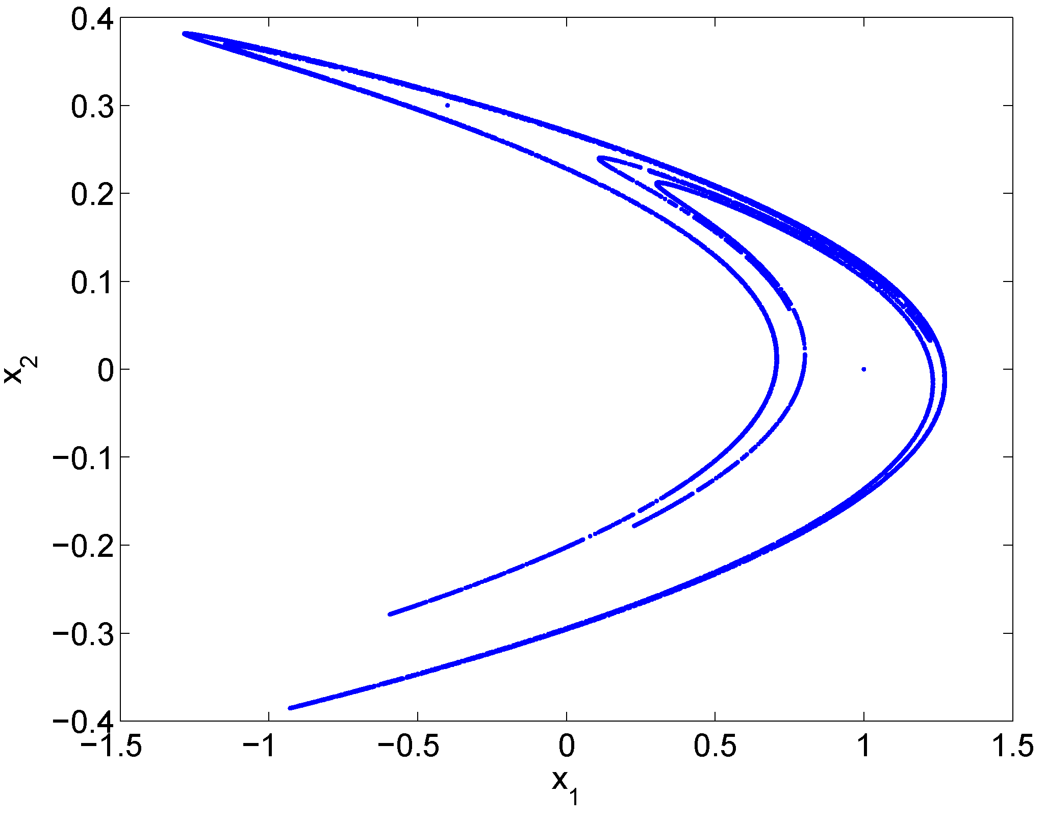
with $a>0$, $b>0$. When $a=1.4$, $b=0.3$, the map is termed “canonical,” for which initially a point will either diverge to infinity, or approach an invariant set known as the H$\acute{\mathrm{e}}$non strange attractor. Shown in Figure 3 is the attractor.

Like the baker transformation, the H$\acute{\mathrm{e}}$non map is invertible, with an inverse

$$\begin{array}{c}\hfill {\Phi }^{-1}(x_1,x_2)=\left(\frac{x_2}{b},x_1-1+\frac{a}{b^2}{x}_2^2\right)\end{array}$$

(66)

The F-P operator thus can be easily found from Equation (18):

$$\begin{array}{ccc}\hfill \mathcal{P}\rho (x_1,x_2)& =& \rho \left({\Phi }^{-1}(x_1,x_2)\right)\left|J^{-1}\right|\hfill \\ & =& \frac{1}{b}·\rho \left(\frac{x_2}{b},x_1-1+\frac{a}{b^2}{x}_2^2\right)\hfill \end{array}$$

(67)

In the following, we compute the flows/transfers between $x_1$ and $x_2$.

Figure 3. A trajectory of the canonical H$\acute{\mathrm{e}}$non map ($a=1.4$, $b=0.3$) starting at $(x_1,x_2)=(1,0)$.

Figure 3. A trajectory of the canonical H$\acute{\mathrm{e}}$non map ($a=1.4$, $b=0.3$) starting at $(x_1,x_2)=(1,0)$.

First, consider $T_{2\to 1}$, i.e., the flow from the linear component $x_2$ to the quadratic component $x_1$. By Equation (23), we need to find the marginal density of $x_1$ at step $\tau +1$ with and without the effect of $x_2$, i.e., ${\left(\mathcal{P}\rho \right)}_1$ and ${\left(\mathcal{P}\rho \right)}_{1\setminus 2}$. With the F-P operator obtained above, ${\left(\mathcal{P}\rho \right)}_1$ is

$$\begin{array}{ccc}\hfill {\left(\mathcal{P}\rho \right)}_1\left(x_1\right)& =& {\int }_{\mathbb{R}}\mathcal{P}\rho (x_1,x_2)d{x}_2\hfill \\ & =& {\int }_{\mathbb{R}}\frac{1}{b}·\rho \left(\frac{x_2}{b},x_1-1+\frac{a}{b}{x}_2^2\right)d{x}_2\hfill \\ & =& {\int }_{\mathbb{R}}\rho (\eta ,x_1-1+a{\eta }^2)d\eta (x_2/b\equiv \eta )\hfill \end{array}$$

If $a=0$, this integral would be equal to ${\rho }_2(x_1-1)$. Note it is the marginal density of $x_2$, but the argument is $x_1-1$. But here $a>0$, the integration is taken along a parabolic curve rather than a straight line. Still the final result will be related to the marginal density of $x_2$; we may as well write it ${\tilde{\rho }}_2\left(x_1\right)$, that is

$$\begin{array}{c}\hfill {\left(\mathcal{P}\rho \right)}_1\left(x_1\right)={\tilde{\rho }}_2\left(x_1\right)\end{array}$$

(68)

Again, notice that the argument is $x_1$.

To compute ${\left({\mathcal{P}}_{\setminus 2}\rho \right)}_1$, let

$$\begin{array}{c}\hfill y_1\equiv {\Phi }_1\left(x_1\right)=1+x_2-a{x}_1^2\end{array}$$

following our convention to distinguish variables at different steps. Modify the system so that $x_2$ is now a parameter. As before, we need to find the counterimage of $(-\infty ,y_1]$ under the transformation with $x_2$ frozen:

$$\begin{array}{c}\hfill {\Phi }_1^{-1}\left((-\infty ,y_1]\right)=\left(-\infty ,-\sqrt{(1+x_2-y_1)/a}\right]\cup \left[\sqrt{(1+x_2-y_1)/a},\infty \right)\end{array}$$

Therefore,

$$\begin{array}{ccc}& & {\left({\mathcal{P}}_{\setminus 2}\rho \right)}_1\left(y_1\right)=\frac{d}{d{y}_1}{\int }_{{\Phi }_1^{-1}\left((-\infty ,y_1]\right)}{\rho }_1\left(s\right)ds\hfill \\ & & =\frac{d}{d{y}_1}{\int }_{-\infty }^{-\sqrt{(1+x_2-y_1)/a}}{\rho }_1\left(s\right)ds+\frac{d}{d{y}_1}{\int }_{\sqrt{(1+x_2-y_1)/a}}^{\infty }{\rho }_1\left(s\right)ds\hfill \\ & & =\frac{1}{2\sqrt{a(1+x_2-y_1)}}\left[{\rho }_1\left(-\sqrt{(1+x_2-y_1)/a}\right)+{\rho }_1\left(\sqrt{(1+x_2-y_1)/a}\right)\right]\hfill \\ & & (y_1<1+x_2)\hfill \\ & & =\frac{1}{2a|x_1|}\left[{\rho }_1(-x_1)+{\rho }_1\left(x_1\right)\right].(\mathrm{recall}{y}_1=1+x_2-a{x}_1^2)\hfill \end{array}$$

Denote the average of ${\rho }_1(-x_1)$ and ${\rho }_1\left(x_1\right)$ as ${\overline{\rho }}_1\left(x_1\right)$ to make an even function of $x_1$. Then ${\left({\mathcal{P}}_{\setminus 2}\rho \right)}_1$ is simply

$$\begin{array}{c}\hfill {\left({\mathcal{P}}_{\setminus 2}\rho \right)}_1\left(y_1\right)=\frac{{\overline{\rho }}_1\left(x_1\right)}{a|x_1|}\end{array}$$

(69)

Note that the parameter $x_2$ does not appear in the arguments. Furthermore, $J_1=det\left(\frac{\partial {\Phi }_1}{\partial x_1}\right)=-2a{x}_1$. Substitute all the above into Equation (23) to get

$$\begin{array}{ccc}\hfill T_{2\to 1}& =& -{\int }_{\mathbb{R}}{\left(\mathcal{P}\rho \right)}_1\left(x_1\right)·log{\left(\mathcal{P}\rho \right)}_1\left(x_1\right)d{x}_1\hfill \\ & & +{\int }_{{\mathbb{R}}^2}{\left({\mathcal{P}}_{\setminus 2}\rho \right)}_1\left(y_1\right)log{\left(\mathcal{P}\rho \right)}_{1\setminus 2}\left(y_1\right)·\rho \left(x_2\right|x_1)·\left|J_1\right|d{x}_{1}d{x}_2\hfill \\ & =& -{\int }_{\mathbb{R}}{\tilde{\rho }}_2\left(x_1\right)log{\tilde{\rho }}_2\left(x_1\right)d{x}_1\hfill \\ & & +{\int }_{\mathbb{R}}\frac{{\overline{\rho }}_1\left(x_1\right)}{a|x_1|}log\frac{{\overline{\rho }}_1\left(x_1\right)}{a|x_1|}·\left|-2a{x}_1\right|·\left[{\int }_{\mathbb{R}}\rho \left(x_2\right|x_1)d{x}_2\right]d{x}_1\hfill \end{array}$$

The taking of the integration with respect to $x_2$ inside the integral is legal since all the terms except the conditional density are independent of $x_2$. With the fact ${\int }_{\mathbb{R}}\rho \left(x_2\right|x_1)d{x}_2=1$, and the introduction of notations $\tilde{H}$ and $\overline{H}$ for the entropy functionals of $\tilde{\rho }$ and $\overline{\rho }$, respectively, we have

$$\begin{array}{c}\hfill T_{2\to 1}={\tilde{H}}_2-2{\overline{H}}_1-log\left|a{x}_1\right|\end{array}$$

(70)

Next, consider $T_{1\to 2}$, the flow from the quadratic component to the linear component. As a common practice, one may start off by computing ${\left(\mathcal{P}\rho \right)}_2$ and ${\left({\mathcal{P}}_{\setminus 1}\rho \right)}_2$. However, in this case, things can be much simplified. Observe that, for the modified system with $x_1$ frozen as a parameter, the Jacobian of the transformation $J_2=det\left[\frac{\partial {\Phi }_2}{\partial x_2}\right]=0.$ So, by Equation (24),

$$\begin{array}{ccc}\hfill T_{1\to 2}& =& -{\int }_{\mathbb{R}}{\left(\mathcal{P}\rho \right)}_2\left(x_2\right)·log{\left(\mathcal{P}\rho \right)}_2\left(x_2\right)d{x}_2\hfill \\ & & +{\int }_{\mathbb{R}}{\left({\mathcal{P}}_{\setminus 1}\rho \right)}_2\left(y_2\right)·log{\left({\mathcal{P}}_{\setminus 1}\rho \right)}_2\left(y_2\right)·\rho \left(x_1\right|x_2)·\left|J_2\right|d{x}_{1}d{x}_2,\hfill \\ & & (y_2\equiv {\Phi }_2(x_1,x_2))\hfill \\ & =& -{\int }_{\mathbb{R}}{\left(\mathcal{P}\rho \right)}_2\left(x_2\right)·log{\left(\mathcal{P}\rho \right)}_2\left(x_2\right)d{x}_2\hfill \end{array}$$

with Equation (67), the marginal density

$$\begin{array}{ccc}\hfill {\left(\mathcal{P}\rho \right)}_2\left(x_2\right)& =& {\int }_{\mathbb{R}}\mathcal{P}\rho (x_1,x_2)d{x}_1\hfill \\ & =& {\int }_{\mathbb{R}}\frac{1}{b}\rho \left(\frac{x_2}{b},x_1-1+a\frac{x_2^2}{b^2}\right)d{x}_1\hfill \\ & =& \frac{1}{b}{\int }_{\mathbb{R}}\rho (y,\xi )d\xi =\frac{1}{b}{\rho }_1\left(\frac{x_2}{b}\right)\hfill \end{array}$$

allowing us to arrive at an information flow from $x_1$ to $x_2$ in the amount of:

$$\begin{array}{ccc}\hfill T_{1\to 2}& =& -{\int }_{\mathbb{R}}\frac{1}{b}{\rho }_1\left(\frac{x_2}{b}\right)·log\left[\frac{1}{b}{\rho }_1\left(\frac{x_2}{b}\right)\right]d{x}_2\hfill \\ & =& H_1+logb\hfill \end{array}$$

(71)

That is to say, the flow from $x_1$ to $x_2$ has nothing to do with $x_2$; it is equal to the marginal entropy of $x_1$, plus a correction term due to the factor b.

The simple result of Equation (71) is remarkable; particularly, if $b=1$, the information flow from $x_1$ to $x_2$ is just the entropy of $x_1$. This is precisely what what one would expect of the mapping component ${\Phi }_2(x_1,x_2)=b{x}_1$ in Equation (65). While the information flow is interesting per se, it also serves as an excellent example for the verification of our formalism.

6.3. Truncated Burgers–Hopf System

In this section, we examine a more complicated system, the Truncated Burgers–Hopf system (TBS hereafter). Originally introduced by Majda and Timofeyev [55] as a prototype of climate modeling, the TBS results from a Galerkin truncation of the Fourier expansion of the inviscid Burgers’ equation, i.e.,

$$\begin{array}{c}\hfill \frac{\partial u}{\partial t}+u\frac{\partial u}{\partial x}=0\end{array}$$

(72)

to the $n^{th}$ order. Liang and Kleeman [51] examined such a system with two Fourier modes retained, which is governed by 4 ordinary differential equations:

$$\begin{array}{ccc}& & \frac{d{x}_1}{dt}=F_1\left(\mathit{x}\right)=x_1{x}_4-x_3{x}_2\hfill \end{array}$$

(73)

$$\begin{array}{ccc}& & \frac{d{x}_2}{dt}=F_2\left(\mathit{x}\right)=-x_1{x}_3-x_2{x}_4\hfill \end{array}$$

(74)

$$\begin{array}{ccc}& & \frac{d{x}_3}{dt}=F_3\left(\mathit{x}\right)=2x_1{x}_2\hfill \end{array}$$

(75)

$$\begin{array}{ccc}& & \frac{d{x}_4}{dt}=F_4\left(\mathit{x}\right)=-x_1^2+x_2^2\hfill \end{array}$$

(76)

Despite its simplicity, the system is intrinsically chaotic, with a strange attractor lying within

$$[-24.8,24.6]\times [-25.0,24.5]\times [-22.3,21.9]\times [-23.7,23.7]$$

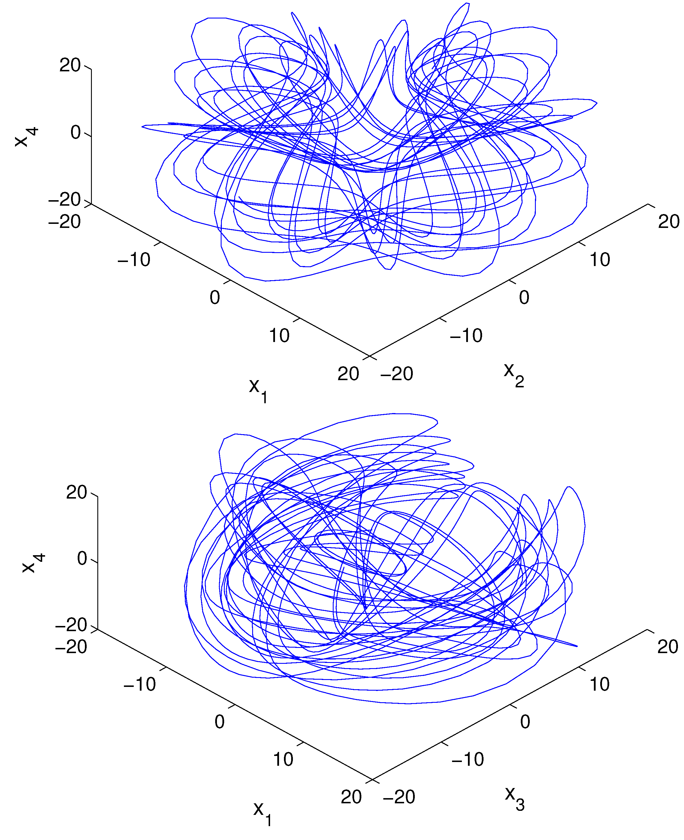
Shown in Figure 4 are its projections onto the $x_1$-$x_2$-$x_4$ and $x_1$-$x_3$-$x_4$ subspaces, respectively.

Finding the information flows within the TBS system turns out to be a challenge in computation, since the Liouville equation corresponding to Equations (73)–(76) is a four-dimensional partial differential equation. In [51], Liang and Kleeman adopt a strategy of ensemble prediction to reduce the computation to an acceptable level. This is summarized in the following steps:

• Initialize the joint density of $(x_1,x_2,x_3,x_4)$ with some distribution ${\rho }_0$; make random draws according to ${\rho }_0$ to form an ensemble. The ensemble should be large enough to resolve adequately the sample space.
• Discretize the sample space into “bins.”
• Do ensemble prediction for the system (73)–(74).
• At each step, estimate the probability density function ρ by counting the bins.
• Plug the estimated ρ back to Equation (39) to compute the rates of information flow at that step.

Figure 4. The invariant attractor of the truncated Burgers–Hopf system (73)–(76). Shown here is the trajectory segment for $2\le t\le 20$ starting at $(40,40,40,40)$. (a) and (b) are the 3-dimensional projections onto the subspaces $x_1$-$x_2$-$x_3$ and $x_2$-$x_3$-$x_4$, respectively.

Figure 4. The invariant attractor of the truncated Burgers–Hopf system (73)–(76). Shown here is the trajectory segment for $2\le t\le 20$ starting at $(40,40,40,40)$. (a) and (b) are the 3-dimensional projections onto the subspaces $x_1$-$x_2$-$x_3$ and $x_2$-$x_3$-$x_4$, respectively.

Notice that the invariant attractor in Figure 4 allows us to perform the computation on a compact subspace of ${\mathbb{R}}^4$. Denote by ${[-d,d]}^4$ the Cartesian product $[-d,d]\times [-d,d]\times [-d,d]\times [-d,d]$. Obviously, ${[-30,30]}^4$ is large enough to cover the whole attractor, and hence can be taken as the sample space. Liang and Kleeman [51] discretize this space into ${30}^4$ bins. With a Gaussian initial distribution $N(\mathbf{\mu },\Sigma )$, where

$$\begin{array}{c}\hfill \mathbf{\mu }=\left[\begin{array}{c}{\mu }_1\hfill \\ {\mu }_2\hfill \\ {\mu }_3\hfill \\ {\mu }_4\hfill \end{array}\right],\Sigma =\left[\begin{array}{cccc}{\sigma }_1^2\hfill & 0\hfill & 0\hfill & 0\hfill \\ 0\hfill & {\sigma }_2^2\hfill & 0\hfill & 0\hfill \\ 0\hfill & 0\hfill & {\sigma }_3^2\hfill & 0\hfill \\ 0\hfill & 0\hfill & 0\hfill & {\sigma }_4^2\hfill \end{array}\right]\end{array}$$

they generate an ensemble of 2,560,000 members, each steered independently under the system (73)–(76). The details about the sample space discretization, probability estimation, etc., are referred to [51]. Shown in the following are only the major results.

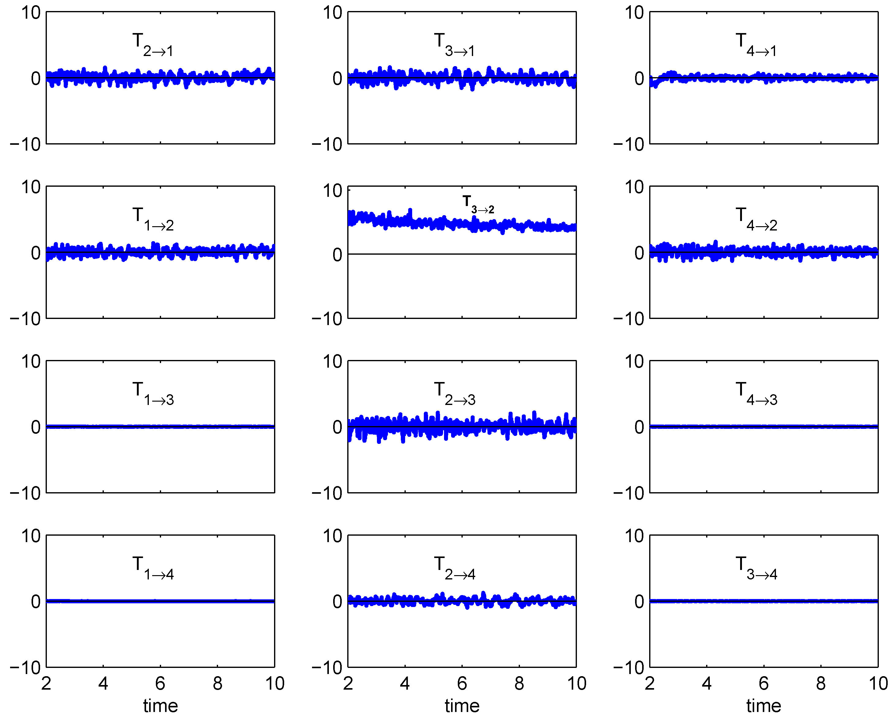
Between the four components of the TBS system, pairwise there are 12 information flows, namely,

$$\begin{array}{ccc}& & T_{2\to 1},T_{3\to 1},T_{4\to 1}\hfill \\ & & T_{1\to 2},T_{3\to 2},T_{4\to 2}\hfill \\ & & T_{1\to 3},T_{2\to 3},T_{4\to 3}\hfill \\ & & T_{1\to 4},T_{2\to 4},T_{3\to 4}\hfill \end{array}$$

To compute these flows, Liang and Kleeman [51] have tried different parameters $\mathbf{\mu }$ and ${\sigma }_k^2$$(k=1,2,3,4)$, but found the final results are the same after $t=2$ when the trajectories are attracted into the invariant set. It therefore suffices to show the result of just one experiment: ${\mu }_k=9$ and ${\sigma }_k^2=9$, $k=1,2,3,4$.

Figure 5. Information flows within the 4D truncated Burgers-Hopf system. The series prior to $t=2$ are not shown because some trajectories have not entered the attractor by that time.

Figure 5. Information flows within the 4D truncated Burgers-Hopf system. The series prior to $t=2$ are not shown because some trajectories have not entered the attractor by that time.

Plotted in Figure 5 are the 12 flow rates. First observe that $T_{3\to 4}=T_{4\to 3}=0$. This is easy to understand, as both $F_3$ and $F_4$ in Equations (75) and (76) have no dependence on $x_3$ nor on $x_4$, implying a zero flow in either direction between the pair ($x_3$, $x_4$) by the property of causality. What makes the result remarkable is, besides $T_{3\to 4}$ and $T_{4\to 3}$, essentially all the flows, except $T_{3\to 2}$, are negligible, although obvious oscillations are found for $T_{2\to 1}$, $T_{3\to 1}$, $T_{1\to 2}$, $T_{4\to 1}$, $T_{2\to 3}$, and $T_{2\to 4}$. The only significant flow, i.e., $T_{3\to 2}$, means that, within the TBS system, it is the fine component that causes an increase in uncertainty in a coarse component but not conversely. Originally the TBS was introduced by Majda and Timofeyev [55] to test their stochastic closure scheme that models the unresolved high Fourier modes. Since additive noises are independent of the state variables, information can only be transferred from the former to the latter. The transfer asymmetry observed here is thus reflected in the scheme.

6.4. Langevin Equation

Most of the applications of information flow/transfer are expected with stochastic systems. Here we illustrate this with a simple 2D system, which has been studied in reference [54] for the validation of Equation (52):

$$\begin{array}{c}\hfill d\mathit{x}=\mathit{A}\mathit{x}dt+\mathit{B}d\mathit{w}\end{array}$$

(77)

where $\mathit{A}=\left(a_{ij}\right)$ and $\mathit{B}=\left(b_{ij}\right)$ are $2\times 2$ constant matrices. This is the linear version of Equation (47). Linear systems are particular in that, if initialized with a normally distributed ensemble, then the distribution of the variables will be a Gaussian subsequently (e.g., [56]). This greatly simplifies the computation which, as we have seen in the previous subsection, is often a formidable task. Let $\mathit{x}\sim N\left(\mathbf{\mu },\Sigma \right)$. Here $\mathbf{\mu }=\left(\begin{array}{c}{\mu }_1\\ {\mu }_2\end{array}\right)$ is the mean vector, and $\Sigma =\left(\begin{array}{cc}{\sigma }_1^2& {\sigma }_{12}\\ {\sigma }_{21}& {\sigma }_2^2\end{array}\right)$ the covariance matrix; they evolve as

$$\begin{array}{ccc}\hfill d\mathbf{\mu }/dt& =& \mathit{A}\mathbf{\mu }\hfill \end{array}$$

(78a)

$$\begin{array}{ccc}\hfill d\Sigma /dt& =& \mathit{A}\Sigma +\Sigma {\mathit{A}}^T+\mathit{B}{\mathit{B}}^T\hfill \end{array}$$

(78b)

($\mathit{B}{\mathit{B}}^T$ is the matrix $\left(g_{ij}\right)$ we have seen in Section 5), which determine the joint density of $\mathit{x}$:

$$\begin{array}{c}\hfill \rho \left(\mathit{x}\right)=\frac{1}{2\pi {\left(det\Sigma \right)}^{1/2}}{e}^{-\frac{1}{2}{(\mathit{x}-\mathbf{\mu })}^T{\Sigma }^{-1}(\mathit{x}-\mathbf{\mu })}\end{array}$$

(79)

By Theorem 5.1, the rates of information flow thus can be accurately computed.

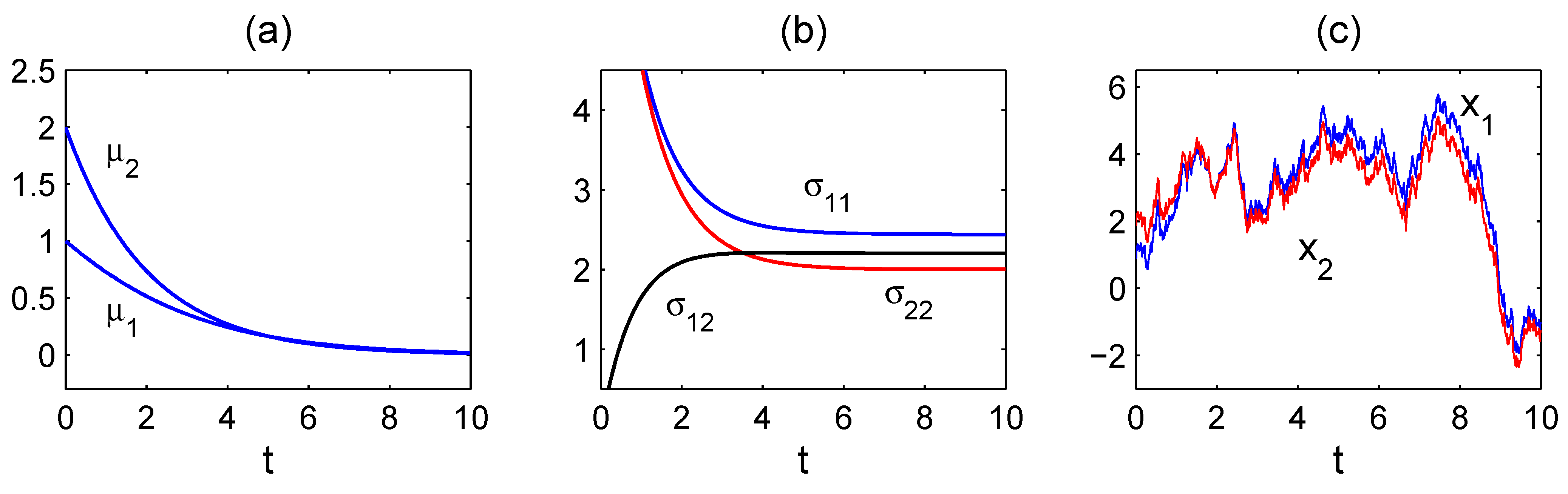
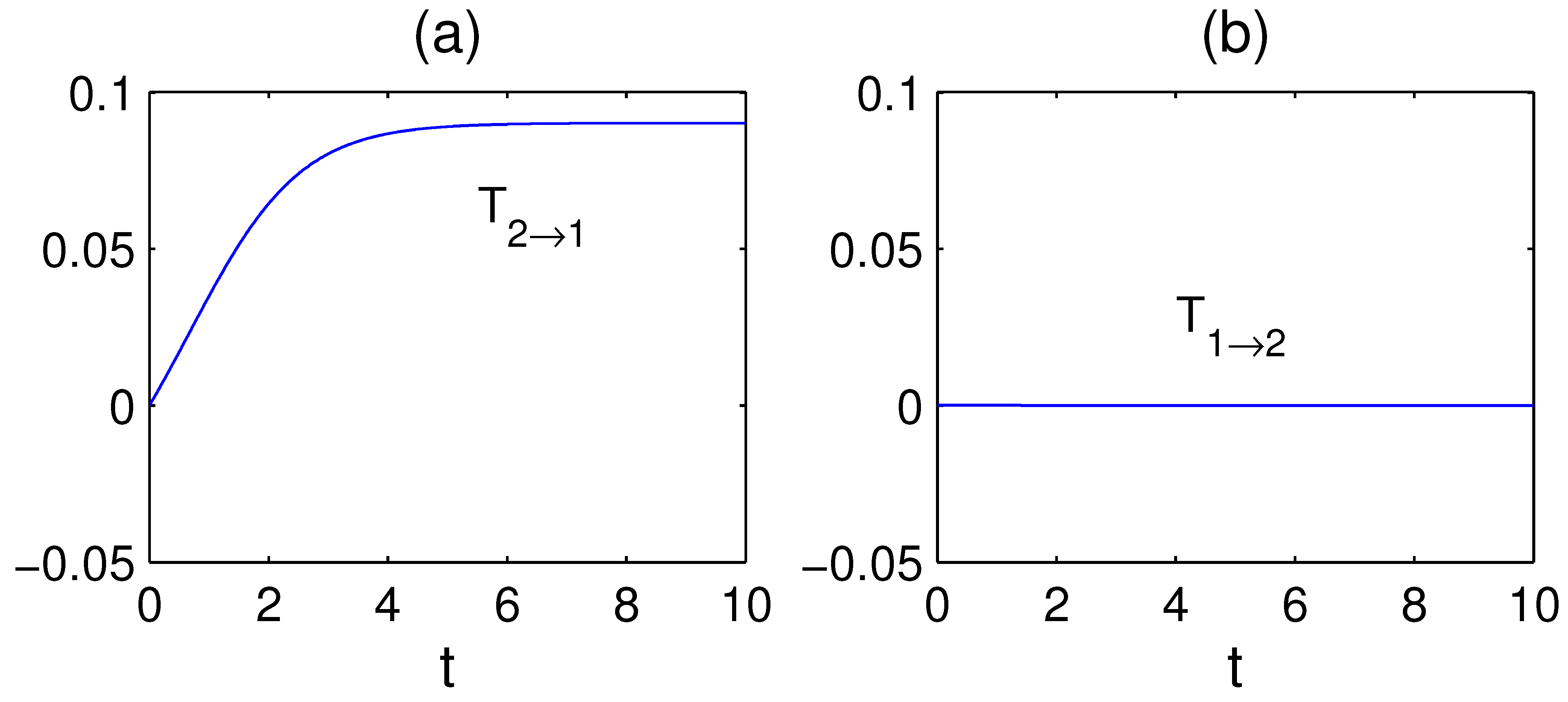
Several sets of parameters have been chosen in [54] to study the model behavior. Here we just look at one such choice: $\mathit{B}=\left(\begin{array}{cc}1& 1\\ 1& 1\end{array}\right)$, $\mathit{A}=\left(\begin{array}{cc}-0.5& 0.1\\ 0& -0.5\end{array}\right)$. Its corresponding mean and covariance approach to an equilibrium: $\mathbf{\mu }\left(\infty \right)=\left(\begin{array}{c}0\\ 0\end{array}\right)$, $\Sigma \left(\infty \right)=\left(\begin{array}{cc}2.44& 2.2\\ 2.2& 2\end{array}\right)$. Shown in Figure 6 are the time evolutions of $\mathbf{\mu }$ and Σ initialized with $\mathbf{\mu }\left(0\right)=\left(\begin{array}{c}1\\ 2\end{array}\right)$ and $\Sigma \left(0\right)=\left(\begin{array}{cc}9\hfill & 0\hfill \\ 0\hfill & 9\hfill \end{array}\right)$, and a sample path of $\mathit{x}$ starting from $(1,2)$. The computed rates of information flow, $T_{2\to 1}$ and $T_{1\to 2}$, are plotted in Figure 7a and b. As time moves on, $T_{2\to 1}$ increases monotonically and eventually approaches a constant; on the other hand, $T_{1\to 2}$ vanishes throughout. While this is within one’s expectations, since $d{x}_2=-0.5x_{2}dt+d{w}_1+dw2$ has no dependence on $x_1$ and hence there should be no transfer of information from $x_1$ to $x_2$, it is interesting to observe that, in contrast, the typical paths of $x_1$ and $x_2$ could be highly correlated, as shown in Figure 6c. In other words, for two highly correlated time series, say $x_1\left(t\right)$ and $x_2\left(t\right)$, one series may have nothing to do with the other. This is a good example illustrating how information flow extends the classical notion of correlation analysis, and how it may be potentially utilized to identify the causal relation between complex dynamical events.

Figure 6. A solution of Equation (78), the model examined in [54], with $a_{21}=0$ and initial conditions as shown in the text: (a) $\mathbf{\mu }$; (b) Σ; and (c) a sample path starting from (1,2).

Figure 6. A solution of Equation (78), the model examined in [54], with $a_{21}=0$ and initial conditions as shown in the text: (a) $\mathbf{\mu }$; (b) Σ; and (c) a sample path starting from (1,2).

Figure 7. The computed rates of information flow for the system (77): (a) $T_{2\to 1}$, (b) $T_{1\to 2}$.

Figure 7. The computed rates of information flow for the system (77): (a) $T_{2\to 1}$, (b) $T_{1\to 2}$.

7. Summary

The past decades have seen a surge of interest in information flow (or information transfer, as it is sometimes called) in different fields of scientific research, mostly in the appearance of some empirical/half-empirical form. We have shown that, given a dynamical system, deterministic or stochastic, this important notion can actually be formulated on a rigorous footing, with flow measures explicitly derived. The general results are summarized in the theorems in Section 3, Section 4 and Section 5. For two-dimensional systems, the result is fairly tight. In fact, if writing such a system as

$$\begin{array}{c}\hfill \left\{\begin{array}{c}d{x}_1=F_1(\mathit{x},t)dt+b_{11}(\mathit{x},t)d{w}_1+b_{12}(\mathit{x},t)d{w}_2\hfill \\ d{x}_2=F_2(\mathit{x},t)dt+b_{21}(\mathit{x},t)d{w}_1+b_{22}(\mathit{x},t)d{w}_2\hfill \end{array}\right.\end{array}$$

where $(w_1,w_2)$ are standard Wiener processes, we have a rate of information flowing from $x_2$ to $x_1$,

$$\begin{array}{c}\hfill T_{2\to 1}=-E\left(F_1\frac{\partial log{\rho }_1}{\partial x_1}\right)-E\left(\frac{\partial F_1}{\partial x_1}\right)+\frac{1}{2}E\left(\frac{1}{{\rho }_1}\frac{{\partial }^2\left(g_{11}{\rho }_1\right)}{\partial x_1^2}\right)\end{array}$$

This is an alternative expression of that in Theorem 5.1; $T_{1\to 2}$ can be obtained by switching the subscripts 1 and 2. In the formula, $g_{11}={\sum }_k{b}_{1k}^2$, ${\rho }_1$ is the marginal density of $x_1$, and E stands for mathematical expectation with respect to ρ, i.e., the joint probability density. On the right-hand side, the third term is contributed by the Brownian notion; if the system is deterministic, this term vanishes. In the remaining two terms, the first is the tendency of $H_1$, namely the marginal entropy of $x_1$; the second can be interpreted as the rate of $H_1$ increase on $x_1$ its own, thanks to the law of entropy production (12) [49], which we restate here:

For an n-dimensional system $\frac{d\mathit{x}}{dt}=\mathit{F}(\mathit{x},t)$, its joint entropy H evolves as $\frac{dH}{dt}=E(\nabla ·\mathit{F})$

This interpretation lies at the core of all the theories along this line. It illustrates that the marginal entropy increase of a component, say, $x_1$, is due to two different mechanisms: the information transferred from some component, say, $x_2$, and the marginal entropy increase associated with a system without taking $x_2$ into account. On this ground, the formalism is henceforth established, with respect to discrete mappings, continuous flows, and stochastic systems, respectively. Correspondingly, the resulting measures are summarized in Equations (24), (39) and (52).

The above-obtained measures possess several interesting properties, some of which one may expect based on daily life experiences. The first one is a property of flow/transfer asymmetry, which has been set as the basic requirement for the identification of causal relations between dynamical events. The information flowing from one event to another event, denoted respectively as $x_2$ and $x_1$, may yield no clue about its counterpart in the opposite direction, i.e., the flow/transfer from $x_1$ to $x_2$. The second says that, if the evolution of $x_1$ is independent of $x_2$, then the flow from $x_2$ to $x_1$ is zero. The third one is about the role of stochasticity, which asserts that, if the stochastic perturbation to the receiving component does not rely on the given component, the flow measure then has a form same as that for the corresponding deterministic system. As a direct corollary, when the noise is additive, then in terms of information flow, the stochastic system functions in a deterministic manner.

The formalism has been put to application with benchmark dynamical systems. In the context of the baker transformation, it is found that there is always information flowing from the stretching direction to the folding direction, while no flow exists conversely. This is in agreement with what one would observe in kneading dough. Application to the H$\acute{\mathrm{e}}$non map also yields a result just as expected on physical grounds. In a more complex case, the formalism has been applied to the study of the scale–scale interaction and information flow between the first two modes of the chaotic truncated Burgers equation. Surprisingly, all the twelve flows are essentially zero, save for one strong flow from the high-frequency mode to the low-frequency mode. This demonstrates that the route of information flow within a dynamical system, albeit seemingly complex, could be simple. In another application, we test how one may control the information flow by tuning the coefficients in a two-dimensional Langevin system. A remarkable observation is that, for two highly correlated time series, there could be no transfer from one certain series, say $x_2$, to the other ($x_1$). That is to say, the evolution of $x_1$ may have nothing to do with $x_2$, even though $x_1$ and $x_2$ are highly correlated. Information flow/transfer analysis thus extends the traditional notion of correlation analysis and/or mutual information analysis by providing a quantitative measure of causality between dynamical events, and this quantification is based firmly on a rigorous mathematical and physical footing.

The above applications are mostly with idealized systems; this is, to a large extent, intended for the validation of the obtained flow measures. Next, we would extend the results to more complex systems, and develop important applications to realistic problems in different disciplines, as envisioned in the beginning of this paper. The scale–scale information flow within the Burgers–Hopf system in § 6.3, for example, may be extended to the flow between scale windows. By a scale window we mean, loosely, a subspace with a range of scales included (cf. [57]). In atmosphere–ocean science, important phenomena are usually defined on scale windows, rather than on individual scales (e.g., [58]). As discussed in [53], the dynamical core of the atmosphere and ocean general circulation models is essentially a quadratically nonlinear system, with the linear and nonlinear operators possessing certain symmetry resulting from some conservation properties (such as energy conservation). Majda and Harlim [53] argue that the state space may be decomposed into a direct sum of scale windows which inherit evolution properties from the quadratic system, and then information flow/transfer may be investigated between these windows. Intriguing as this conceptual model might be, there still exist some theoretical difficulties. For example, the governing equation for a window may be problem-specific; there may not be such governing equations as simply written as those like Equation (3) for individual components. Hence one may need to seek new ways to the derivation of the information flow formula. Nonetheless, central at the problem is still the aforementioned classification of mechanisms that govern the marginal entropy evolution; we are expecting new breakthroughs along this line of development.

The formalism we have presented thus far is with respect to Shannon entropy, or absolute entropy as one may choose to refer to it. In many cases, such as in the El Niño case where predictability is concerned, this may need to be modified, since the predictability of a dynamical system is measured by relative entropy. Relative entropy is also called Kullback–Leibler divergence; it is defined as

$$\begin{array}{c}\hfill D(\rho \parallel q)=E_{\rho }\left[log\left(\frac{\rho }{q}\right)\right]\end{array}$$

i.e., the expectation of the logarithmic difference between a probability ρ and another reference probability q, where the expectation is with respect to ρ. Roughly it may be interpreted as the “distance” between ρ and q, though it does not satisfy all the axioms for a distance functional. Therefore, for a system, if letting the reference density be the initial distribution, its relative entropy at a time t informs how much additional information is added (rather than how much information it has). This provides a natural choice for the measure of the utility of a prediction, as pointed out by Kleeman (2002) [59]. Kleeman also argues in favor of relative entropy because of its appealing properties, such as nonnegativity and invariance under nonlinear transformations [60]. Besides, in the context of a Markov chain, it has been proved that it always decreases monotonically with time, a property usually referred to as the generalized second law of thermodynamics (e.g., [60,61]). The concept of relative entropy is now a well-accepted measure of predictability (e.g., [59,62]). When predictability problems (such as those problems in atmosphere-ocean science and financial economics as mentioned in the introduction) are dealt with, it is necessary to extend the current formalism to one with respect to the relative entropy functional. For all the dynamical system settings in this review, the extension should be straightforward.

References

- Baptista, M.S.; Garcia, S.P.; Dana, S.K.; Kurths, J. Transmission of information and synchronization in a pair of coupled chaotic circuits: An experimental overview. Eur. Phys. J.-Spec. Top. 2008, 165, 119–128. [Google Scholar] [CrossRef]
- Baptista, M.D.S.; Kakmeni, F.M.; Grebogi, C. Combined effect of chemical and electrical synapses in Hindmarsh-Rose neural networks on synchronization and the rate of information. Phys. Rev. E 2010, 82, 036203. [Google Scholar] [CrossRef] [PubMed]
- Bear, M.F.; Connors, B.W.; Paradiso, M.A. Neuroscience: Exploring the Brain, 3rd ed.; Lippincott Williams & Wilkins: Baltimore, MD, USA, 2007; p. 857. [Google Scholar]
- Vakorin, V.A.; MiAiA, B.; Krakovska, O.; McIntosh, A.R. Empirical and theoretical aspects of generation and transfer of information in a neuromagnetic source network. Front. Syst. Neurosci. 2011, 5, 96. [Google Scholar] [CrossRef] [PubMed]
- Ay, N.; Polani, D. Information flows in causal networks. Advs. Complex Syst. 2008, 11. [Google Scholar] [CrossRef]
- Peruani, F.; Tabourier, L. Directedness of information flow in mobile phone communication networks. PLoS One 2011, 6, e28860. [Google Scholar] [CrossRef] [PubMed]
- Sommerlade, L.; Amtage, F.; Lapp, O.; Hellwig, B.; Licking, C.H.; Timmer, J.; Schelter, B. On the estimation of the direction of information flow in networks of dynamical systems. J. Neurosci. Methods 2011, 196, 182–189. [Google Scholar] [CrossRef] [PubMed]
- Donner, R.; Barbosa, S.; Kurths, J.; Marwan, N. Understanding the earth as a complex system-recent advances in data analysis and modelling in earth sciences. Eur. Phys. J. 2009, 174, 1–9. [Google Scholar] [CrossRef]
- Kleeman, R. Information flow in ensemble weather prediction. J. Atmos. Sci. 2007, 64, 1005–1016. [Google Scholar] [CrossRef]
- Materassi, M.; Ciraolo, L.; Consolini, G.; Smith, N. Predictive space weather: An information theory approach. Adv. Space Res. 2011, 47, 877–885. [Google Scholar] [CrossRef]
- Tribbia, J.J. Waves, Information and Local Predictability. In Proceedings of the Workshop on Mathematical Issues and Challenges in Data Assimilation for Geophysical Systems: Interdisciplinary Perspectives, IPAM, UCLA, 22–25 February 2005.
- Chen, C.R.; Lung, P.P.; Tay, N.S.P. Information flow between the stock and option markets: Where do informed traders trade? Rev. Financ. Econ. 2005, 14, 1–23. [Google Scholar] [CrossRef]
- Lee, S.S. Jumps and information flow in financial markets. Rev. Financ. Stud. 2012, 25, 439–479. [Google Scholar] [CrossRef]
- Sommerlade, L.; Eichler, M.; Jachan, M.; Henschel, K.; Timmer, J.; Schelter, B. Estimating causal dependencies in networks of nonlinear stochastic dynamical systems. Phys. Rev. E 2009, 80, 051128. [Google Scholar] [CrossRef] [PubMed]
- Zhao, K.; Karsai, M.; Bianconi, G. Entropy of dynamical social networks. PLoS One 2011. [Google Scholar] [CrossRef] [PubMed]
- Cane, M.A. The evolution of El Niño, past and future. Earth Planet. Sci. Lett. 2004, 164, 1–10. [Google Scholar] [CrossRef]
- Jin, F.-F. An equatorial ocean recharge paradigm for ENSO. Part I: conceptual model. J. Atmos. Sci. 1997, 54, 811–829. [Google Scholar] [CrossRef]
- Philander, S.G. El Niño, La Niña, and the Southern Oscillation; Academic Press: San Diego, CA, USA, 1990. [Google Scholar]
- Ghil, M.; Chekroun, M.D.; Simonnet, E. Climate dynamics and fluid mechanics: Natural variability and related uncertainties. Physica D 2008, 237, 2111–2126. [Google Scholar] [CrossRef]
- Mu, M.; Xu, H.; Duan, W. A kind of initial errors related to “spring predictability barrier” for El Niño events in Zebiak-Cane model. Geophys. Res. Lett. 2007, 34, L03709. [Google Scholar] [CrossRef]
- Zebiak, S.E.; Cane, M.A. A model El Niño-Southern Oscillation. Mon. Wea. Rev. 1987, 115, 2262–2278. [Google Scholar] [CrossRef]
- Chen, D.; Cane, M.A. El Niño prediction and predictability. J. Comput. Phys. 2008, 227, 3625–3640. [Google Scholar] [CrossRef]
- Mayhew, S.; Sarin, A.; Shastri, K. The allocation of informed trading across related markets: An analysis of the impact of changes in equity-option margin requirements. J. Financ. 1995, 50, 1635–1654. [Google Scholar] [CrossRef]
- Goldenfield, N.; Woese, C. Life is physics: Evolution as a collective phenomenon far from equilibrium. Ann. Rev. Condens. Matt. Phys. 2011, 2, 375–399. [Google Scholar] [CrossRef]
- K¨ppers, B. Information and the Origin of Life; MIT Press: Cambridge, UK, 1990. [Google Scholar]
- Murray, J.D. Mathematical Biology; Springer-Verlag: Berlin, Germany, 2000. [Google Scholar]
- Allahverdyan, A.E.; Janzing, D.; Mahler, G. Thermodynamic efficiency of information and heat flow. J. Stat. Mech. 2009, PO9011. [Google Scholar] [CrossRef]
- Crutchfield, J.P.; Shalizi, C.R. Thermodynamic depth of causal states: Objective complexity via minimal representation. Phys. Rev. E 1999, 59, 275–283. [Google Scholar] [CrossRef]
- Davies, P.C.W. The Physics of Downward Causation. In The Re-emergence of Emergence; Clayton, P., Davies, P.C.W., Eds.; Oxford University Press: Oxford, UK, 2006; pp. 35–52. [Google Scholar]
- Ellis, G.F.R. Top-down causation and emergence: Some comments on mechanisms. J. R. Soc. Interface 2012, 2, 126–140. [Google Scholar] [CrossRef] [PubMed]
- Okasha, S. Emergence, hierarchy and top-down causation in evolutionary biology. J. R. Soc. Interface 2012, 2, 49–54. [Google Scholar] [CrossRef] [PubMed]
- Walker, S.I.; Cisneros, L.; Davies, P.C.W. Evolutionary transitions and top-down causation. arXiv:1207.4808v1 [nlin.AO], 2012. [Google Scholar]
- Wu, B.; Zhou, D.; Fu, F.; Luo, Q.; Wang, L.; Traulsen, A. Evolution of cooperation on stochastic dynamical networks. PLoS One 2010, 5, e11187. [Google Scholar] [CrossRef] [PubMed]
- Pope, S. Turbulent Flows, 8th ed.; Cambridge University Press: Cambridge, UK, 2011. [Google Scholar]
- Faes, L.; Nollo, G.; Erla, S.; Papadelis, C.; Braun, C.; Porta, A. Detecting Nonlinear Causal Interactions between Dynamical Systems by Non-uniform Embedding of Multiple Time Series. In Proceedings of the Engineering in Medicine and Biology Society, Buenos Aires, Argentina, 31 August–4 September 2010; pp. 102–105.
- Kantz, H.; Shreiber, T. Nonlinear Time Series Analysis; Cambridge University Press: Cambridge, UK, 2004. [Google Scholar]
- Schindler-Hlavackova, K.; Palus, M.; Vejmelka, M.; Bhattacharya, J. Causality detection based on information-theoretic approach in time series analysis. Phys. Rep. 2007, 441, 1–46. [Google Scholar] [CrossRef]
- Granger, C. Investigating causal relations by econometric models and cross-spectral methods. Econometrica 1969, 37, 424–438. [Google Scholar] [CrossRef]
- McWilliams, J.C. The emergence of isolated, coherent vortices in turbulence flows. J. Fluid Mech. 1984, 146, 21–43. [Google Scholar] [CrossRef]
- Salmon, R. Lectures on Geophysical Fluid Dynamics; Oxford University Press: Oxford, UK, 1998; p. 378. [Google Scholar]
- Bar-Yam, Y. Dynamics of Complex Systems; Addison-Welsley Press: Reading, MA, USA, 1997; p. 864. [Google Scholar]
- Crutchfield, J.P. The calculi of emergence: computation, dynamics, and induction induction. “Special issue on the Proceedings of the Oji International Seminar: Complex Systems-From Complex Dynamics to Artifical Reality”. Physica D 1994, 75, 11–54. [Google Scholar] [CrossRef]
- Goldstein, J. Emergence as a construct: History and issues. Emerg. Complex. Org. 1999, 1, 49–72. [Google Scholar] [CrossRef]
- Corning, P.A. The re-emergence of emergence: A venerable concept in search of a theory. Complexity 2002, 7, 18–30. [Google Scholar] [CrossRef]
- Vastano, J.A.; Swinney, H.L. Information transport in sptiotemporal systems. Phys. Rev. Lett. 1988, 60, 1773–1776. [Google Scholar] [CrossRef] [PubMed]
- Kaiser, A.; Schreiber, T. Information transfer in continuous processes. Physica D 2002, 166, 43–62. [Google Scholar] [CrossRef]
- Schreiber, T. Measuring information transfer. Phys. Rev. Lett. 2000, 85, 461. [Google Scholar] [CrossRef] [PubMed]
- Liang, X.S.; Kleeman, R. A rigorous formalism of information transfer between dynamical system components. I. Discrete mapping. Physica D 2007, 231, 1–9. [Google Scholar] [CrossRef]
- Liang, X.S.; Kleeman, R. Information transfer between dynamical system components. Phys. Rev. Lett. 2005, 95, 244101. [Google Scholar] [CrossRef] [PubMed]
- Lasota, A.; Mackey, M.C. Chaos, Fractals, and Noise: Stochastic Aspects of Dynamics; Springer: New York, NY, USA, 1994. [Google Scholar]
- Liang, X.S.; Kleeman, R. A rigorous formalism of information transfer between dynamical system components. II. Continuous flow. Physica D 2007, 227, 173–182. [Google Scholar] [CrossRef]
- Liang, X.S. Uncertainty generation in deterministic fluid flows: Theory and applications with an atmospheric stability model. Dyn. Atmos. Oceans 2011, 52, 51–79. [Google Scholar] [CrossRef]
- Majda, A.J.; Harlim, J. Information flow between subspaces of complex dynamical systems. Proc. Natl. Acad. Sci. USA 2007, 104, 9558–9563. [Google Scholar] [CrossRef]
- Liang, X.S. Information flow within stochastic dynamical systems. Phys. Rev. E 2008, 78, 031113. [Google Scholar] [CrossRef] [PubMed]
- Majda, A.J.; Timofeyev, I. Remarkable statistical behavior for truncated Burgers-Hopf dynamics. Proc. Natl. Acad. Sci. USA 2000, 97, 12413–12417. [Google Scholar] [CrossRef] [PubMed]
- Gardiner, C.W. Handbook of Stochastic Methods for Physics, Chemistry, and the Natural Sciences; Springer-Verlag: Berlin/Heidelberg, Germany, 1985. [Google Scholar]
- Liang, X.S.; Anderson, D.G.M.A. Multiscale window transform. SIAM J. Multiscale Model. Simul. 2007, 6, 437–467. [Google Scholar] [CrossRef]
- Liang, X.S.; Robinson, A.R. Multiscale processes and nonlinear dynamics of the circulation and upwelling events off Monterey Bay. J. Phys. Oceanogr. 2009, 39, 290–313. [Google Scholar] [CrossRef]
- Kleeman, R. Measuring dynamical prediction utility using relative entropy. J. Atmos. Sci. 2002, 59, 2057–2072. [Google Scholar] [CrossRef]
- Cover, T.M.; Thomas, J.A. Elements of Information Theory; Wiley: New York, NY, USA, 1991. [Google Scholar]
- Ao, P. Emerging of stochastic dynamical equalities and steady state thermodynamics from Darwinian dynamics. Commun. Theor. Phys. 2008, 49, 1073–1090. [Google Scholar] [CrossRef] [PubMed]
- Tang, Y.; Deng, Z.; Zhou, X.; Cheng, Y.; Chen, D. Interdecadal variation of ENSO predictability in multiple models. J. Clim. 2008, 21, 4811–4832. [Google Scholar] [CrossRef]
© 2013 by the authors; licensee MDPI, Basel, Switzerland. This article is an open access article distributed under the terms and conditions of the Creative Commons Attribution license (http://creativecommons.org/licenses/by/3.0/).
Share and Cite
MDPI and ACS Style
Liang, X.S. The Liang-Kleeman Information Flow: Theory and Applications. Entropy 2013, 15, 327-360. https://doi.org/10.3390/e15010327
AMA Style
Liang XS. The Liang-Kleeman Information Flow: Theory and Applications. Entropy. 2013; 15(1):327-360. https://doi.org/10.3390/e15010327
Chicago/Turabian StyleLiang, X. San. 2013. "The Liang-Kleeman Information Flow: Theory and Applications" Entropy 15, no. 1: 327-360. https://doi.org/10.3390/e15010327