Article

Symmetry-Based Balance Equation for Local Entropy Density in a Dissipative Multibaker Chain System

Department of Mechanical Science and Bioengineering, Osaka University, 1-3 Machikaneyama,Toyonaka, Osaka 560-8531, Japan
Entropy 2013, 15(10), 4345-4375; https://doi.org/10.3390/e15104345
Submission received: 5 August 2013 / Revised: 24 September 2013 / Accepted: 9 October 2013 / Published: 16 October 2013
(This article belongs to the Special Issue Advances in Methods and Foundations of Non-Equilibrium Thermodynamics)

Abstract

:
In this study, the balance equation for local entropy density defined on each partition is obtained by the decomposition of the time-evolution operator for local entropy density, on the level of the master equation, by using symmetric and antisymmetric properties for the inversion of partition, density pairs and a given drift velocity. The resultant equation includes the following terms: convection, diffusion, entropy flow due to a thermostat and entropy production. The averaging of the four terms recover the corresponding terms in a balance equation for the macroscopic entropy density of irreversible thermodynamics for a thermostated system. Moreover, an empirical law of order estimation is introduced to explain the limiting behavior of the averaged quantities in the macroscopic limit for the bulk system. The law makes it possible to separate some minor contributions from the major four terms and, for example, to explain the positive entropy production rate in a nonequilibrium state for volume-preserving systems, even if the state is far from steady state. They are numerically confirmed on an invertible, dissipative multibaker chain system, named a circuit model. These properties are independent of partitioning.

1. Introduction

The macroscopic irreversibility and positive entropy production induced by reversible microscopic dynamics has been a major problem in nonequilibrium statistical mechanics. It is well known that the Boltzmann entropy and the Gibbs entropy, both of which are successfully applied to equilibrium statistical mechanics, pose problems for the nonequilibrium state. For example, the Gibbs entropy, defined by the absolute continuous probability measure, has the essential problem in the nonequilibrium state that it is kept constant in a closed system relaxing towards equilibrium and decreases with a constant rate in an open system towards a non-equilibrium steady state. This is related to the fact that a deterministic thermostating system leads to a fractal probability measure [1,2,3,4], and it is widely accepted, therefore, that a coarse-grained entropy (ε-entropy) must be introduced [5,6,7,8,9,10,11,12,13,14,15,16,17,18,19,20,21,22]. That is why the coarse-grained dynamics is essential for the statistical interpretations that are consistent with irreversible thermodynamics.
In general, the balance equation for the coarse-grained entropy change consists of three terms: entropy flow, entropy flow due to the thermostat and nonnegative entropy production [5]. A similar equation and its extended form are utilized by Vollmer, Breymann and Mátyás et al. [6,7,8,18,19,20]. Gilbert and Dorfman [5] derived an entropy balance equation on dissipative systems and applied its formalism to a dyadic multibaker chain that mimics a system with enforcing flux through bulk dissipation. The coarse-grained entropy production on each site is identified with the phenomenological entropy production in the infinite system limit. Vollmer and Breymann et al. [6,7] showed that a similar formalism recovers the results of thermodynamics, including the irreversible entropy production rate by choosing appropriate transfer rates on a triadic multibaker chain. Vollmer and Mátyás et al. [18,19,20,22] also proposed a coarse-grained entropy and an entropy balance equation, both of which depend on the kinetic energy density or the temperature and, thereby, recovered cross effects, such as the Peltier and Zeebeck effects.
These balance equations are derived by the decomposition of a quantity, entropy change, based on the physical meaning of each term. However, the reasoning about specifying the contribution of entropy flow due to a thermostat is not necessarily clear. It is actually contaminated by a component of a flux term, i.e., a term attributed to a surface integral when integrated on a region, even though it should be macroscopically a source term. The flux component can be observed for some entropy-flow or entropy-flow-like variables, due to a thermostat, even in the macroscopic limit [5,6] (cf. Section 2). In addition, the decomposition does not allow us to subdivide the entropy flow term into convection and diffusion terms. It shows the limitations for utilizing a physical decomposition to find a coarse-grained form corresponding to an arbitrary macroscopic quantity when, for example, a system is driven by complex external fields.
In the present paper, we shall consider another, completely different way to find the coarse-grained expression. We shall decompose the equation for the coarse-grained or local entropy density defined on each partition into four terms that consists of convection, diffusion, entropy flow due to a thermostat and entropy production. It can be interpreted as the mathematical decomposition, not of the quantity of entropy change, but of the time-evolution operator of the local entropy density on the level of the master equation based on the symmetric and antisymmetric properties for some inversions. The decomposition is complete in the sense that the averaging of each term of the equation over a macroscopic small region recovers the corresponding one in the balance equation for the macroscopic entropy density. This is an extension of the previous study [10] for volume-preserving systems, whose decomposition is not applicable to dissipative systems. The procedure is in principle applicable to any balance equations, including the entropy balance.
Moreover, we shall also consider an empirical law of order estimation (LOE). It allows us to estimate the order of a given averaged quantity for the scale parameter, Δ, of partitions. The above-mentioned form of the balance equation cannot explain the positivity of the entropy production rate in nonequilibrium states, and therefore, further decomposition of the entropy production term into nonnegative and remaining terms is required. It turns out that the order of the remaining term is very important. Ishida [10] shows that the entropy source term in the volume-preserving system consists of a nonnegative term and a residual term. The law explains that the former remains of order one ( O ( 1 ) ) and the latter vanishes in the macroscopic limit as Δ 0 . Thus, the estimation law is responsible for the law of increasing entropy in an isolated system. This extends the comprehensive discussion of Vollmer [22] on the nonphysical, higher-order contributions to the discrete entropy balance. It also provides physical insights on what are non-vanishing, observable, macroscopic variables composed of microscopic ones.
In this study, these ideas are numerically validated on a deterministic, reversible and dissipative multibaker chain system, called a circuit model, which is an extended model that generalizes the original one proposed by Vollmer, Tél and Mátyás (Model III in [18]). By selecting a different transfer rate in a single cell, the model mimics a system with an enforcing flow driven by a thermostat on a boundary. We shall also numerically confirm that these findings are independent of coarse-graining, partitioning parameters. This is an essential feature for coarse-grained statistics [7,13].
In the present approach, the macroscopic small region, or site, is partitioned by a Markov partition with arbitrary resolution described by a bit or trit number, d. Eventually, we numerically confirm that the averaged quantities and their orders are independent of the resolution parameter d. This is along the line of discussions by Gaspard, Gilbert and Barra et al. [5,11,12,13,14,15,16,17,21]. In addition, the multibaker model introduced in the present study is based on the triadic multibaker chain that has been utilized by Vollmer, Tél and Mátyás et al. [6,7,8,9,18,19,20,22]. The partitioning of d = 1 corresponds to their level-0 partitioning. Thus, the present study brings together, in a unified manner, various approaches from previous research.

2. Symmetry and Decomposition of the Equation for Local Entropy Density

In the following, we have a balance equation for local entropy density whose terms correspond to the macroscopic ones when averaged appropriately. That is to say, each term gives a local or coarse-grained expression for a corresponding macroscopic quantity. The decomposition is based on symmetric and anti-symmetric properties for the inversion of the partition pair (i,j), the density pair ( ρ i , ρ j ) and a given drift velocity, as summarized in Table 1, referring to the property of the macroscopic equation for entropy density. In this process, an empirical law of order estimation is introduced to estimate the limiting behavior of the averaged quantities. Eventually, the discussion of this study is confined to be a multibaker chain system. In this section, however, we do not utilize a form specific to the multibaker chain, but follow a form based on the master equation [10] in order to maintain its applicability to other dissipative systems, e.g., jump processes [23].
Table 1. Symmetry property of each term in the local entropy density equation.
TypeInversionSymmetric termAntisymmetric term
(i)partition pair (i, j)sourceflux
(ii)sign of drift v for flux termdiffusionconvection
(iii)density pair ( ρ i , ρ j ) and (ii) for source termproductionflow due to a thermostat

2.1. Two Symmetry Properties and the Decomposition of an Equation for Local Probability Density

We begin with a master equation for the local, coarse-grained probability density ρ, defined on each partition. If we follow the notation of Ishida [10], the equation can be written as:
Δ V i Δ ρ i ( n ) Δ V i ( ρ i ( n + 1 ) ρ i ( n ) ) = P i ( n + 1 ) P i ( n ) j J j i ( n ) Δ i , j = j 1 Δ i , j U ˜ j i ρ i ( n ) + ρ j ( n ) 2 D ˜ i , j Δ i , j ( ρ j ( n ) ρ i ( n ) )
where Δ V i denotes the Liouville measure or volume of the ith partition, P i ( n ) the probability measure on the ith partition at the nth time step, ρ i ( n ) ( P i ( n ) / Δ V i ) the local probability density and J j i ( n ) the probability flux from the ith to the jth partition. U ˜ j i and D ˜ i , j are, respectively, the velocity-like and diffusion-coefficient-like variables defined by:
U ˜ j i ( W ˜ j i W ˜ i j ) Δ i , j , D ˜ i , j W ˜ j i + W ˜ i j 2 Δ i , j 2
where W ˜ j i , called the transition volume, is defined as W j i Δ V i by use of the transition probability, W j i , from the ith to jth partition. Δ i , j ( = Δ j , i ) is a characteristic distance between the ith and jth partition, reflecting the distance between the two partitions. It is worth noting that its precise definition does not affect the following formulation, but that the distance plays an essential or symbolic role on the estimation of the order of averaged coarse-grained quantities on a macroscopic small region. In this estimation, Δ i , j is required to be of the order Δ 1 ( O ( Δ ) ), where Δ is a scale parameter reflecting the maximum distance between the possible ith and jth partitions and determining a macroscopic limit as Δ 0 . The estimation is discussed later. In Equation (1), the sum means the summation with respect to all of the jth partition, whose W i j or W j i is not zero. For this equation, such a restriction of j is unnecessary. However, it is essential for some equations in this study (cf. Equation (20)).
In Equations (1) and (2), the subscript “ j i “ indicates a directional quantity, which is antisymmetric for the interchange of a partition pair, i and j. On the other hand, the subscript “i,j” indicates a non-directional quantity, which is symmetric for the interchange. In what follows, we utilize these notations for the inversion. Considering that D ˜ i , j and U ˜ j i are symmetric and anti-symmetric, respectively, for the interchange, we can easily find that the summand of the rightmost term of Equation (1) is anti-symmetric. When Equation (1) is summed with respect to the ith partition included in a region, R, most of the summands cancel out, and Equation (1) reduces to the summation on its surface, vanishing for the whole space R. Consequently, the summation of the probability measure is kept constant. The property can be regarded as the local, coarse-grained form of the divergence theorem of Gauss. Thus, the local expression of macroscopic flux or advection-diffusion terms must be anti-symmetric. It follows that a macroscopic source term should be expressed by a symmetric term. These properties allow us to decompose arbitrary local, coarse-grained terms into flux and source terms.
It is well known that for a dynamical system to realize a nonequilibrium steady state that is driven by a thermostat, it should be dissipative [2,3,4,5,6,7,8]. A resultant drift is associated with a volume expansion rate, and the drift velocity vanishes if the rate is unity [4,6,7]. Therefore, we can expect that the transition volume, W ˜ j i , is divided into symmetric W ˜ j i [ s ] and antisymmetric W ˜ j i [ a ] parts for the inversion of the drift with the aid of a local volume expansion rate property, e i , at the ith partition, defined as:
e i = Δ V i / k W ˜ i k = k W ˜ k i / k W ˜ i k
As we shall see in Section 3, the parts can be expressed, at least for most multibaker chain systems, as:
W ˜ j i [ s ] = ( 1 + e j ) W ˜ j i / 2 , W ˜ j i [ a ] = ( 1 e j ) W ˜ j i / 2
In what follows, the superscripts, [s] and [a], indicate that the quantity is symmetric and antisymmetric for the inversion of drift, respectively.
It is not so important to understand the form of Equation (4) at this point, considering that the decomposition itself is always possible. Let v be a parameter of the macroscopic intensity of the external field, e.g., the drift velocity. Then, the transition volume is a function of v, and we obtain:
W ˜ j i [ s ] = ( W ˜ j i ( v ) + W ˜ j i ( v ) ) / 2 , W ˜ j i [ a ] = ( W ˜ j i ( v ) W ˜ j i ( v ) ) / 2
Once these transition volumes are given, Equation (1) can be decomposed into two terms :
Δ V i Δ ρ i ( n ) = j J j i [ a ] ( n ) Δ i , j j J j i [ s ] ( n ) Δ i , j
where:
J j i [ a ] ( n ) U ˜ j i [ a ] ρ j ( n ) + ρ i ( n ) 2 D ˜ i , j [ a ] Δ i , j ( ρ j ( n ) ρ i ( n ) )
U ˜ j i [ a ] ( W ˜ j i [ a ] W ˜ i j [ a ] ) Δ i , j , D ˜ i , j [ a ] W ˜ j i [ a ] + W ˜ i j [ a ] 2 Δ i , j 2
and their symmetric counterparts, J j i [ s ] ( n ) , U ˜ j i [ s ] and D ˜ i , j [ s ] , can be similarly defined.
The first and second terms of Equation (5a) are antisymmetric and symmetric for the inversion of the drift, respectively. Therefore, these terms can be local expressions of convection and diffusion terms in a macroscopic equation for probability density, i.e., the Fokker-Planck equation. If we take an appropriate macroscopic small region, R, we can introduce a kind of averaging on R for a volume, time-dependent local, coarse-grained quantity, A i ( n ) , as follows:
A R ( n ) = 1 τ Δ V R i R A i ( n )
where Δ V R denotes the volume of the region R, τ the time increment (time step) of a given map and i R indicates that the quantity, A i ( n ) , is summed with respect to all the partitions included in the region R. Please note that the two terms in Equation (5a) depend on both the time step and the volume of the ith and jth partitions through the transition volume (4). As a whole, the averaging of Equation (1) leads to the increasing rate of macroscopic density [5,6,7,8,9,10,11,12,13,14,15,16,17]. Although the details are not given here, we can numerically confirm that the two right-hand-side (RHS) terms in Equation (5a) are averaged to, respectively, the convection and diffusion terms in the Fokker-Planck equation for the multibaker chain introduced in Section 3. It is worthwhile noting that J j i [ a ] ( n ) vanishes when a given multibaker map is volume-preserving, because e i = e j = 1 in this case. This is in agreement with the arguments of Vollmer, Tél and Breymann, who state that transports in thermostating systems cannot be described by Hamiltonian systems [6,7].

2.2. Decomposition of Equation for Local Entropy Density

In this section, we deal with a balance equation for local entropy density, whose terms are averaged to correspond with those in the following equation for the macroscopic entropy density, s, of nonequilibrium thermodynamics:
s t = S e , m a c + S s , m a c
where:
S e , m a c · J s = · ( s v ρ v ) · ( D s ) S c , m a c + S d , m a c
S s , m a c j 2 ρ D j · v D S p , m a c + S t h , m a c
s ρ ln ( ρ / ρ r ) , J s 1 + ln ( ρ / ρ r ) j , j ρ v D ρ
Herein, ρ r , a constant, denotes a reference density, v the drift velocity and D the diffusion coefficient. Note that S s , m a c is the macroscopic entropy source, not the symmetric part of the macroscopic change of entropy density. In this paper, symmetric and antisymmetric properties appear in the superscript inside the brackets.
Firstly, substituting the Taylor series up to second order into Δ ϕ i ( n ) ( ϕ ( ρ i ( n + 1 ) ) ϕ ( ρ i ( n ) ) ) the equation for a function, ϕ ( ρ i ( n ) ) , can be decomposed into the following leading and residual terms:
Δ V i Δ ϕ i ( n ) Δ V i ( ϕ ( ρ i ( n + 1 ) ) ϕ ( ρ i ( n ) ) ) = Δ V i Δ ρ i ( n ) ϕ ( ρ i ( n ) ) + O ( Δ ρ i 2 ) Δ V i
we can take the following form of the equation for the local entropy density:
Δ V i Δ s i ( n ) Δ V i ( s i ( n + 1 ) s i ( n ) ) = Δ V i Δ ρ i ( n ) 1 + ln ( ρ i ( n ) / ρ r ) + r T , i ( n )
where:
( local entropy density ) s i ( n ) ρ i ( n ) ln ( ρ i ( n ) / ρ r )
( transient residual ) r T , i ( n ) 2 Δ V i ρ i ( n + 1 ) ln ρ i ( n + 1 ) ln ρ i ( n ) 2 Δ ρ i ( n ) 2 ρ i ( n + 1 )
As the averaging of Equation (1), as is done in Equation (6), agrees with the increasing rate of the macroscopic probability density, Δ ρ is of the order τ, and therefore, the averaged residual is also of the order τ. It vanishes in the macroscopic limit. Herein, it should be noted that the leftmost term of Equation (9a), called the unsteady term, is summed over a given macroscopic small region R to agree with the change of the so-called coarse-grained entropy on R. Thus, the formalism is in line with coarse-grained statistics [5,6,7,8,9,10,11,12,13,14,15,16,17].
Substituting the following identity:
j T i j ( n ) j 1 Δ i , j ( U ˜ j i [ s ] + 2 D ˜ i , j [ a ] Δ i , j ) ρ i ( n ) = 0
and Equation (1) into Equation (9a) and considering the symmetry property for the interchange of a partition pair, i and j, gives:
Δ V i Δ s i ( n ) = j J j i ( n ) Δ i , j 1 + ln ( ρ i ( n ) / ρ r ) T i j ( n ) + r T , i ( n ) = j J j i ( n ) Δ i , j 1 + ln ( ρ j ( n ) / ρ r ) + ln ( ρ i ( n ) / ρ r ) 2 J j i [ s ^ ] ( n ) Δ i , j + j J j i ( n ) Δ i , j ln ρ j ( n ) ln ρ i ( n ) 2 + 1 Δ i , j U ˜ j i [ s ] ρ j ( n ) ρ i ( n ) 2 D ˜ i , j [ a ] Δ i , j ( ρ j ( n ) + ρ i ( n ) ) + r T , i ( n ) S e , i ( n ) + S s , i ( n ) + r T , i ( n )
where:
J j i [ s ^ ] ( n ) U ˜ j i [ s ] ρ j ( n ) + ρ i ( n ) 2 D ˜ i , j [ a ] Δ i , j ( ρ j ( n ) ρ i ( n ) )
is a probability flux, which is symmetric for the simultaneous inversion of the drift and a density pair ( ρ i , ρ j ). Its antisymmetric counterpart, J j i [ a ^ ] ( n ) , is given by:
J j i [ a ^ ] ( n ) U ˜ j i [ a ] ρ j ( n ) + ρ i ( n ) 2 D ˜ i , j [ s ] Δ i , j ( ρ j ( n ) ρ i ( n ) )
These terms with superscripts [ a ^ ] and [ s ^ ] should not be confused with J j i [ s ] ( n ) and J j i [ a ] ( n ) , which are based only on the symmetric property for the drift inversion. The summands in S e , i ( n ) and S s , i ( n ) are antisymmetric and symmetric for the interchange of a partition pair, i and j, respectively. Since the two components are unique when a summand is given as the first part of Equation (11), S e , i ( n ) and S s , i ( n ) must be the flux term and the source term, respectively. The former is related to the macroscopic flux, S e , m a c (7b), and the latter is related to the macroscopic source, S s , m a c (7c). The additional terms originating from the identity (10) play an essential role as described later.
Similar to Equation (5a), the flux term, S e , i ( n ) , can be decomposed into the following terms:
S e , i ( n ) = j J j i [ a ] ( n ) Δ i , j 1 + ln ( ρ j ( n ) / ρ r ) + ln ( ρ i ( n ) / ρ r ) 2 + D ˜ i , j [ a ] Δ i , j 2 ( ρ j ( n ) ρ i ( n ) ) + j J j i [ s ] ( n ) Δ i , j 1 + ln ( ρ j ( n ) / ρ r ) + ln ( ρ i ( n ) / ρ r ) 2 U ˜ j i [ s ] Δ i , j ρ j ( n ) + ρ i ( n ) 2 = S ^ c , i ( n ) + S ^ d , i ( n )
The first and second terms of the equation are, respectively, antisymmetric and symmetric for the inversion of the drift, corresponding, in turn, to the convection and diffusion in the equation for the local entropy density. We will numerically validate the decomposition in Section 3.
It is natural, therefore, for us to expect that the entropy source term, S s , i ( n ) , can also be divided into two terms based on the symmetry property for the same inversion and that the two terms are associated with the macroscopic entropy source, S s , m a c , of the form diffusion plus convection:
S s , m a c = D ρ ρ 2 v · ρ S s d , m a c + S s c , m a c
However, this assumption is not correct. Ishida [10] shows that unsteady macroscopic entropy production in a volume-preserving system has the following property in the macroscopic limit:
A R ( n ) S s , m a c = D ρ ρ 2
where:
A i ( n ) j D ˜ i , j Δ i , j 2 ( ρ j ( n ) ρ i ( n ) ) 2 ρ j ( n ) + ρ i ( n ) = j D ˜ i , j [ s ] Δ i , j 2 ( ρ j ( n ) ρ i ( n ) ) 2 ρ j ( n ) + ρ i ( n )
and R is a site in a multibaker chain. As we shall see, however, we can numerically confirm that Equation (14a) does not hold for the dissipative system introduced in Section 3. Considering that the summand is linear with respect to the transition probability and that both U ˜ j i [ a ] and D ˜ i , j [ a ] vanish in a volume-preserving system, the extension, A e , i ( n ) , of Equation (14b) for the dissipative system must be of the form:
A e , i ( n ) = j D ˜ i , j [ s ] Δ i , j 2 ( ρ j ( n ) ρ i ( n ) ) 2 ρ j ( n ) + ρ i ( n ) + U ˜ j i [ a ] B j i ( n ) + D ˜ i , j [ a ] C i , j ( n )
Thus, the addend cannot be symmetric for the inversion of the drift. That is the reason why the symmetric component of S s , i ( n ) for the drift inversion is not in accord with S s d , m a c . The entropy source, S s , i ( n ) , must be divided on another basis.
The basis is heuristic to some extent. The entropy source, S s , i ( n ) , consists of the contributions between the possible partition pairs (see Equation (11)). In a contribution between a partition pair (i,j), the component of the entropy production can be deduced to be unchanged if the sign of the drift velocity, v, and a density pair ( ρ i , ρ j ) are inverted simultaneously, because the production would depend only on the scalar variables between the two partitions, independent of its direction. On the other hand, it is natural for us to assume that the component of the entropy flow, due to the thermostat, is antisymmetric for the simultaneous inversion. It follows that the entropy source, S s , i ( n ) , is decomposed as follows:
S s , i ( n ) = j J j i [ a ^ ] ( n ) Δ i , j ln ρ j ( n ) ln ρ i ( n ) 2 + j J j i [ s ^ ] ( n ) Δ i , j ln ρ j ( n ) ln ρ i ( n ) 2 + 1 Δ i , j U ˜ j i [ s ] ρ j ( n ) ρ i ( n ) 2 D ˜ i , j [ a ] Δ i , j ( ρ j ( n ) + ρ i ( n ) ) (15) S ^ p , i ( n ) + S ^ t h , i ( n )
Herein, notice that J j i [ s ^ ] ( n ) and J j i [ a ^ ] ( n ) are, respectively, symmetric and anti-symmetric for the simultaneous inversion of the drift and a density pair ( ρ i , ρ j ). The summands of the first and second terms in Equation (15) are as a whole symmetric and antisymmetric for the simultaneous inversion, respectively. These observations imply that the first and second terms of Equation (15) are related to, respectively, macroscopic entropy production, S p , m a c , and macroscopic entropy flow due to the thermostat, S t h , m a c . The decomposition is also numerically validated in Section 3. Thus, the decomposition of the equation for the local entropy density corresponding to the macroscopic Equation (7) is completed. The above procedures are summarized in Table 1.
The balance equation of the local entropy density, Equations (11), (13) and (15), is based only on symmetry properties, except for the separation of r T . Therefore, we can expect that the form is effective for many systems. For example, it is capable of explaining a macroscopic entropy flux density into the thermostat on the boundary (cf. Section 3). However, it poses an essential problem, i.e., we cannot know whether the averaged quantity of S ^ p , i ( n ) , corresponding to the macroscopic entropy production, is nonnegative. Further decomposition of the term is, therefore, needed to separate a nonnegative contribution from a remaining term. In the next section, we will find that the remaining term is averaged to vanish in the macroscopic limit by use of an empirical law of order estimation and some numerical experiments. In the course of the decomposition, we will see that the balance equation reaches a comprehensible form that is similar to its macroscopic form, Equation (7).

2.3. Order Estimation, Residuals and Positivity of Entropy Production Rate

Ishida [10] proposes a balance equation for the local entropy density with the nonnegative entropy production term and two residual terms. In a volume-preserving multibaker chain system, the averaging of the entropy production term is theoretically shown to converge to the macroscopic entropy production. On the other hand, the averaged quantities of the two residuals are numerically confirmed to vanish in the macroscopic limit. To date, these numerical observations, including the present dissipative cases, are limited to the case where D, v and a partitioning parameter, β, described later, are constant in the bulk system, but lead to the following empirical law of order estimation:
Law of order estimation (LOE): Let a local, coarse-grained quantity, A i j ( n ) , be a product of the power of the primary order components shown in Table 2 and be linear with the transition volume. That is to say, A i j ( n ) has the form:
A i j ( n ) = U ˜ j i [ ] × B i j ( n ) or A i j ( n ) = D ˜ i , j [ ] × C i j ( n )
and B i j ( n ) and C i j ( n ) exclude U ˜ j i [ ] or D ˜ i , j [ ] . The power index of an antisymmetric order component, shown in Table 2, must be nonnegative. Then, for a scale parameter, Δ, that represents the maximum distance between the ith and jth partitions, Δ i , j , and for an appropriate macroscopic small region R in a given phase space, the order, m, of the averaged quantity, A R ( n ) ( O ( Δ m ) ) , for a local quantity, A i ( n ) j A i j ( n ) , is the summation of the quantity of the order of each component, shown in Table 2, times its power index, if (a) A i j ( n ) is symmetric for the interchange of the partition pair, i and j, or (b) the order is the quantity plus one.
Table 2. Primary order components.
OrderSymmetric* order componentsAntisymmetric* order components
0C (a constant), D ˜ i , j [ s ] , U ˜ j i [ a ] , U ˜ j i [ s ] , ρ j ( n ) ρ i ( n ) Δ i , j
ln ρ j ( n ) + ρ i ( n ) 2 , ρ j ( n ) + ρ i ( n ) 2 ,
ln ρ j ( n ) + ln ρ i ( n ) 2 * *
1 Δ i , j ln ρ j ( n ) ln ρ i ( n ) 2 * * , ρ j ( n ) ρ i ( n ) ρ j ( n ) + ρ i ( n ) * *
2 D ˜ i , j [ a ]
(*) The symmetric property is based on the interchange of partition pair i and j; (**) The order of this component can be deduced from other components.
For example, we shall obtain the order, m, of the averaged quantity for the following:
A i ( n ) j A i j ( n ) j D ˜ i , j [ s ] ρ j ( n ) ρ i ( n ) Δ i , j l
When l is an even number, the summand, A i j ( n ) , is symmetric for the interchange of the partition pair, i and j, and we have m = 0 + 0 × l = 0 , where the first zero in the RHS of the equation is the order of D ˜ i , j [ s ] . If, conversely, l is an odd number, the summand is antisymmetric, and therefore m = 0 + 0 × l + 1 = 1 . Thus, the averaged quantity behaves like O ( Δ 0 ) of O ( Δ 1 ) , dependent on l.
The empirical law shows that the averaged quantity of each term in the EquationS (5a), (13) and (15) is of the zeroth order ( O ( Δ 0 ) ) or order one, converging to a value in the macroscopic limit as Δ 0 , and the quantity is observed as a macroscopic one. We can also deduce that the averaged term, including the component, D ˜ i , j [ a ] , in Equation (13), is of the order Δ 2 , vanishing in the macroscopic limit.
The law also provides the following preferred decompositions of the symmetric S s , i ( n ) and antisymmetric S e , i ( n ) terms that are intuitively comprehensible.
First, the flux term, S e , i ( n ) , can be decomposed into the following three terms:
S e , i ( n ) = S c , i ( n ) + S d , i ( n ) + r e , i ( n )
where:
( convection ) S c , i ( n ) j J s , j i [ a ] ( n ) Δ i , j + j J j i [ a ] ( n ) Δ i , j
( diffusion ) S d , i ( n ) j J s , j i [ s ] ( n ) Δ i , j
( residual entropy flux ) r e , i ( n ) j U ˜ j i 2 Δ i , j ( ρ j ( n ) ρ i ( n ) ) 2 ρ j ( n ) + ρ i ( n ) j U ˜ j i Δ i , j ρ j ( n ) ρ i ( n ) 2 D ˜ i , j Δ i , j 2 ( ρ j ( n ) + ρ i ( n ) ) l j i ( n ) + j 2 D ˜ i , j [ a ] Δ i , j 2 ( ρ j ( n ) ρ i ( n ) )
J s , j i [ a ] ( n ) U ˜ j i [ a ] s j ( n ) + s i ( n ) 2 D ˜ i , j [ a ] s j ( n ) s i ( n ) Δ i , j
J s , j i [ s ] ( n ) U ˜ j i [ s ] s j ( n ) + s i ( n ) 2 D ˜ i , j [ s ] s j ( n ) s i ( n ) Δ i , j
l j i ( n ) ln ρ j ( n ) ln ρ i ( n ) 2 ρ j ( n ) ρ i ( n ) ρ j ( n ) + ρ i ( n )
Herein, J s indicates the local entropy density flux. The term (18d) can be regarded as an extension of the antisymmetric residual term in volume-preserving systems [10] to the one in dissipative systems. Using the following identity:
ln y ln x 2 = m = 0 1 2 m + 1 y x y + x 2 m + 1 for x , y > 0
for the term l j i ( n ) , Equation (18g), we can estimate the order of the averaged quantity of Equation (18d) as the order Δ 2 from the estimation law.
As long as the residual has a vanishing order, the remaining terms, S c , i ( n ) and S d , i ( n ) , are of the order one from the order of Equation (13). The summands in S c , i ( n ) and S d , i ( n ) are, respectively, antisymmetric and symmetric for the inversion of the drift, corresponding to the first and second terms of Equation (13). Referring to Equation (5a), the new terms, Equations (18b) and (18c), have local forms corresponding to Equation (7b).
Second, the symmetric source term, S s , i ( n ) , can be decomposed as follows:
S s , i ( n ) = ( S p , i ( n ) + r p , i ( n ) ) + ( S t h , i ( n ) + r t h , i ( n ) ) + r s , i ( n )
where:
( entropy production ) S p , i ( n ) j J j i [ a ^ ] ( n ) 2 ( ρ j ( n ) + ρ i ( n ) ) D ˜ i , j [ s ]
( entropy flow due to a thermostat ) S t h , i ( n ) j J j i [ s ^ ] ( n ) U ˜ j i [ a ] 2 D ˜ i , j [ s ]
( minor entropy production ) r p , i ( n ) j J j i [ a ^ ] ( n ) U ˜ j i [ a ] 2 D ˜ i , j [ s ]
( minor entropy flow due to a thermostat ) r t h , i ( n ) j J j i [ a ^ ] ( n ) J j i [ s ^ ] ( n ) ( ρ j ( n ) + ρ i ( n ) ) D ˜ i , j [ s ] + 1 Δ i , j U ˜ j i [ s ] ρ j ( n ) ρ i ( n ) 2 D ˜ i , j [ a ] Δ i , j ( ρ j ( n ) + ρ i ( n ) )
( residual entropy source ) r s , i ( n ) j J j i ( n ) Δ i , j l j i ( n )
Similarly, the averaged residual entropy source (20f), identical to the symmetric residual term in volume-preserving systems [10], is of the order Δ 2 , and, therefore ( S p , i ( n ) + r p , i ( n ) ) and ( S t h , i ( n ) + r t h , i ( n ) ) are of the order one from the order of Equation (15). These leading terms are symmetric and anti-symmetric for the simultaneous inversion of the drift and a density pair ( ρ i , ρ j ), respectively, corresponding to the first and second terms of Equation (15). Note also that their major components, S p , i ( n ) , Equation (20b), and S t h , i ( n ) , Equation (20c), have similar forms to Equation (7c), and therefore, it is natural for us to expect that their minor components of r p , i ( n ) , Equation (20d), and r t h , i ( n ) , Equation (20e), do nothing on the macroscopic level. As we shall see, we can numerically confirm that their averaged quantities are of the order Δ 2 and vanish in the macroscopic limit, though we cannot estimate the order by the estimation law.
The local expression of entropy production (20b) is always positive in non-equilibrium states, and the above-mentioned nature of the component (20d) is responsible for the positivity of the macroscopic entropy production. For the case of volume-preserving systems, the terms, (20c), (20d) and (20e) vanish, and Ishida [10] shows that the positivity depends on the behavior of the residual term (20f) vanishing in the macroscopic limit. Now, the law of order estimation can explain this quantity, and therefore, we can ascertain that it is responsible for the positive entropy production for the systems and, therefore, the law of increasing entropy in an isolated system.
Moreover, the following relation for the entropy flow due to a thermostat:
S ^ t h , i ( n ) S t h , i ( n ) + r t h , i ( n ) = j J j i [ s ^ ] ( n ) Δ i , j ρ j ( n ) ρ i ( n ) ρ j ( n ) + ρ i ( n ) + 1 Δ i , j U ˜ j i [ s ] ρ j ( n ) ρ i ( n ) 2 D ˜ i , j [ a ] Δ i , j ( ρ j ( n ) + ρ i ( n ) )
allows us to interpret an additional term that originates from the identity, Equation (10), i.e., the second term of the summand of the Equation (21). The first term of the summand involves a symmetric term for the inversion of the drift, which remains even for the volume-preserving cases in which the flow, Equation (21), should vanish. The additional term is interpreted as the elimination of the symmetric term and the inclusion of an alternative antisymmetric term, which is also antisymmetric for the simultaneous inversion of drift and a density pair ( ρ i , ρ j ) and, at the same time, symmetric for the inversion of a partition pair (i, j) (cf. Table 1).
Finally, it would be useful to compare this formalism with the conventional balance equation for the coarse-grained entropy on multibaker chain systems introduced by Gilbert, Dorfman and Gaspard [5] from the viewpoint of symmetry. It is possible for us to interpret the conventional equation as the following form for the local entropy density:
Δ V i Δ s i ( t ) = Δ e S i ( t ) + Δ t h S i ( t ) + Δ i S i ( t )
where:
Δ e S i ( t ) j W ˜ i j s j ( t ) Δ V i s i ( t ) = j 1 Δ i , j ( J s , j i [ a ] ( t ) + J s , j i [ s ] ( t ) )
Δ t h S i ( t ) j W ˜ i j ρ j ( t ) ln k W ˜ i k Δ V i
Δ i S i ( t ) j W ˜ i j ρ j ( t ) ln ρ j ( t ) k W ˜ i k ρ i ( t + 1 ) Δ V i
Herein, Δ e S i ( t ) denotes the entropy flux, Δ t h S i ( t ) the entropy flow due to the thermostats, and Δ i S i ( t ) the internal entropy production. The RHS of Equation (22d) is nonnegative and positive in a non-equilibrium state.
We find that the summands in Equations (22c) and (22d) are neither symmetric nor anti-symmetric for the interchange of a partition pair (i, j). That is why these local, coarse-grained forms are not desirable for expressing the macroscopic entropy source (7c). In fact, Vollmer, Tél and Breymann [6] show that the averaging of (22c) involves a part of the entropy flux, S c , m a c (7b), in addition to the macroscopic entropy flow due to a thermostat, S t h , m a c (7c), as discussed later. In contrast, the averaged quantity of Equation (22d) agrees with the macroscopic entropy production, S p , m a c (7c), and therefore, we can say that the antisymmetric part of the summand of Equation (22d) behaves like a residual term that vanishes in the macroscopic limit. It should be stressed, therefore, that not the inherent positive form of Equation (22d), but the vanishing behavior of the residual term is responsible for the positivity of the macroscopic entropy production in a nonequilibrium state.

3. Circuit Model: A Multibaker Chain System-

In the following, let us consider a multibaker chain system, called a circuit model, to numerically validate the formalism in the previous section. The circuit-like, time-reversal model, slightly modified from the triadic multibaker chain proposed by Vollmer, Tél and Mátyás [18], realizes a nonequilibrium steady state by a thermostated boundary, which mimics the action of a battery. Its macroscopic unsteady state obeys the Fokker-Planck equation by use of which we can compare each evolving term in the macroscopic balance equation, Equation (7), for the entropy density with its corresponding averaged term in the balance equation for the local entropy density, as mentioned above. We will also numerically analyze the behavior of the residual and minor terms in the macroscopic limit.

3.1. Introduction of a Multibaker Chain System and the Conventional Formalism

The multibaker chain consists of N rectangular sites of width Δ r ( = l / N ) and height h. The length, l, is the total length of the chain, determining the typical length for the sites to span in a given direction. At each time step, the nth square site, A n , is divided into three vertical columns numbered from ω=0 (leftmost) to two (rightmost). That is why the map is called a triadic multibaker chain system. The ωth strip of width η n ( ω ) Δ r and height, h, is to be mapped onto the ωth horizontal strip of width Δ r and height ν m ( ω ) h on the m ( = n 1 + ω ) th site, A m . The summation of η n ( ω ) and ν n ( ω ) with respect to ω are unity for the site, 1 n N . Such a map T can be described as:
T ( n , x , y ) = ( n 1 , x / η n ( 0 ) , ν n 1 ( 0 ) y ) , 0 x < η n ( 0 ) Δ r , ( n , ( x η n ( 0 ) Δ r ) / η n ( 1 ) , ν n ( 0 ) h + ν n ( 1 ) y ) , η n ( 0 ) Δ r x < ( η n ( 0 ) + η n ( 1 ) ) Δ r , ( n + 1 , [ x ( η n ( 0 ) + η n ( 1 ) ) Δ r ] / η n ( 2 ) , ( η n ( 0 ) + η n ( 1 ) ) Δ r ( ν n + 1 ( 0 ) + ν n + 1 ( 1 ) ) h + ν n + 1 ( 2 ) y ) , x Δ r ,
where (n,x,y) denotes a position (x,y) on the nth site; the map is defined in the range 0 x Δ r and 0 y h . The origin is fixed at the lower left corner of each site, and the coordinates, x and y, are the horizontal and vertical direction, respectively.
The site A n is partitioned by disjoint 3 d horizontal cells, identified by ω ̲ d ( ω 0 ω 1 ω d 1 ) , where ω k = 0, 1 or 2. The partitioning is based on the fact that the SRB (Sinai-Ruelle-Bowen) measure [1] is smooth in the unstable direction [13,24]. The quantity, ω ̲ d , can be regarded as a ternary number, and each cell of width Δ r by height h × ν n ( ω ̲ d ) forms a line in its numerical order from bottom to top. Then, d, independent of n, is interpreted as a trit number expressing the resolution of the partitioning. Hereafter, a partition identified by the number on the nth site is denoted by ( n , ω ̲ d ) .
Now, let us introduce the following vertical position, y ( n , ω ̲ d ) :
y ( n , ω ̲ d ) h i = 0 d 1 ν n ( ω ̲ i ) ω = 0 ω i 1 ν n + Δ ( ω ̲ i ) ( ω )
where:
ν n ( ω ̲ i ) k = 0 i 1 ν n + Δ ( ω ̲ k ) ( ω k ) , ν n ( ω ̲ 0 ) 1 , Δ ( ω ̲ k ) l = 0 k 1 ( 1 ω l ) , Δ ( ω ̲ 0 ) 0
The above-mentioned partitioning leads to a Markov partition [21,24] when the vertical range of the partition ( n , ω ̲ d ) is arranged to be y ( n , ω ̲ d ) y y ( n , ω ̲ d + 1 ) , where ω ̲ d + 1 denotes the ternary number obtained by the addition of one to the number ω ̲ d . Note that the height, h ν n ( ω ̲ d ) , of the partition can be expressed as:
h ν n ( ω ̲ d ) = y ( n , ω ̲ d + 1 ) y ( n , ω ̲ d )
Herein, appropriate boundary conditions are needed so that the site number m= n + Δ ( ω ̲ k ) in Equation (24) can be defined, even if the number is outside the range of 1 m N , described later.
The condition for a dissipative chain system to be consistent with non-equilibrium thermodynamics requires that η n ( ω ) = ν n ( 2 ω ) [6,7], and such a map is found to be invertible in the sense that it has a time-reversal operator R, defined as R ( n , x , y ) = ( n , Δ r ( 1 y / h ) , h ( 1 x / Δ r ) ) , such that R 2 = 1 and the reversed map T 1 can be described as T 1 = R T R .
The definition (24) can be utilized to define a region ( n , ω ̲ k ) where k is a positive integer and the region is a partition like the ones mentioned above if k = d . The region has the area of Δ V ( n , ω ̲ k ) ( h Δ r ν n ( ω ̲ k ) ) , and the equation for the probability measure on the region can be expressed as:
P ( t + 1 ) ( n , ω ̲ k ) = η n + 1 ω 0 ( ω 0 ) P ( t ) ( n + 1 ω 0 , ω ̲ k 1 ) = ω k = 0 2 η n + 1 ω 0 ( ω 0 ) P ( t ) ( n + 1 ω 0 , ω ̲ k 1 ω k )
where P ( t ) ( n , ω ̲ k ) denotes the probability measure at the tth step in the region ( n , ω ̲ k ) , and ω ̲ k 1 ω 1 ω k 1 . This equation shows that η n + 1 ω 0 ( ω 0 ) corresponds to the transition probability, W i j . If all of the 3 d N partitions in the N sites are numbered and the ith corresponding measure, P, at the tth step is denoted by P i ( t ) , then Equation (26) for k=d can be rewritten in the form of Equation (1). Thus, we have the form of the balance Equations (11), (18) and (20) for local entropy density specific to this multibaker chain system.
Ishida [10] and Vollmer et al. [6,7,8,9] introduced a triadic multibaker chain system whose macroscopic measure (probability) density ρ is governed by the one-dimensional Fokker-Planck equation, namely:
ρ t + r ρ v D ρ r = 0 for 0 r l
When v and D are uniform in the bulk system, the macroscopic density profile is microscopically realized by the following transition probability, which is independent of site number n for 1 n N 1 :
η ( 0 ) = 1 2 ( 2 τ Δ r 2 D τ Δ r v ) , η ( 2 ) = 1 2 ( 2 τ Δ r 2 D + τ Δ r v ) , η ( 1 ) = 1 η ( 0 ) η ( 2 )
where D(>0) denotes the diffusion coefficient, v the drift velocity and τ ( > 0 ) the time step. For the case of v 0 , the bulk system becomes dissipative. The transfer rate has the property that η ( 0 ) = η ( 2 ) = 0 when τ = 0 . This property of the triadic multibaker model is the key to realizing a convergent macroscopic density profile that is governed by the Fokker-Planck equation [5,7]. As described later, a different transfer rate is imposed on the boundary site A N .
When the probability η corresponding to the transition probability W i j is thus defined, it is straightforward to confirm that:
e j ( r ) = 1 / e j , W j i ( r ) = e j W j i
for the inversion of the drift, i.e., the sign of the drift velocity, v, where e j ( r ) and W j i ( r ) are the expansion rate and transition probability for the inverted map, respectively. As a result, the symmetric and antisymmetric parts of the transition volume W ˜ j i are identified as Equation (4).
Considering that the transition probability (28) can be rewritten as:
η ( 0 ) = β 2 ( 1 P e g 2 ) , η ( 2 ) = β 2 ( 1 + P e g 2 ) , η ( 1 ) = 1 β
the condition that η ( ω ) should be positive yields:
0 < β < 1 , | P e g | < 2
where β 2 τ D / Δ r 2 and P e g ( v Δ r / D ) is the so-called grid Péclet number [25]. Therefore, the time step τ must be greater than or equal to the order of Δ r 2 . In this study, the order is taken to be Δ r 2 , so that β is constant [10].
For comparison, let us consider here the formulation proposed by Gilbert, Dorfman and Gaspard [5] in which the time change of the coarse-grained entropy, Δ S ( t ) , at a site, A n , based on the partition, ω ̲ d , is divided into entropy flux Δ e S ( t ) , entropy flow due to a thermostat, Δ t h S ( t ) , and internal entropy production, Δ i S ( t ) . A similar formalism has also been utilized by Vollmer, Tél and Breymann [6]. Applying the formulation to the present multibaker chain in which both ν and η depend on site n, we obtain the following balance equation:
Δ S ( t ) = Δ e S ( t ) + Δ t h S ( t ) + Δ i S ( t )
where:
Δ e S ( t ) ω ̲ d + 1 P ( t + 1 ) ( n , ω ̲ d + 1 ) ln P ( t + 1 ) ( n , ω ̲ d + 1 ) ρ r η n + 1 ω 0 ( ω 0 ) Δ V ( n + 1 ω 0 , ω ̲ d ) (31b) + ω ̲ d P ( t ) ( n , ω ̲ d ) ln P ( t ) ( n , ω ̲ d ) ρ r Δ V ( n , ω ̲ d )
Δ t h S ( t ) ω ̲ d + 1 P ( t + 1 ) ( n , ω ̲ d + 1 ) ln η n + 1 ω 0 ( ω 0 ) ν n ( ω 0 )
Δ i S ( t ) ω ̲ d + 1 P ( t + 1 ) ( n , ω ̲ d + 1 ) ln ν n + 1 ω 0 ( ω ̲ d ) P ( t + 1 ) ( n , ω ̲ d ) ν n + 1 ω 0 ( ω ̲ d 1 ) P ( t + 1 ) ( n , ω ̲ d + 1 )
Substituting Equation (26) into Equation (31), we can easily find its local, coarse-grained form, Equation (22), such that:
Δ S ( t ) = i A n Δ V i Δ s i ( t ) , Δ e S ( t ) = i A n Δ e S i ( t )
and so on. Herein, i A n means the sum of a quantity over the partitions included in the site, A n , and the summation divided by τ h Δ r is in accord with the definition of the averaging, Equation (6), on a macroscopic small region, A n . Vollmer, Tél and Breymann [6] theoretically show that the averaged quantities have the following convergent properties:
Δ e S A n ( t ) J s r r ( ρ v )
Δ t h S A n ( t ) j v D + r ( ρ v )
Δ i S A n ( t ) j 2 ρ D
as N ( = l / Δ r ) , where:
J s 1 + ln ( ρ / ρ r ) j , j ( ρ v D ρ r )
The macroscopic quantities appearing on the RHS of Equation (33) should be evaluated at a macroscopic position, r n Δ r , and at a macroscopic time, t m τ t . It should be stressed here that the property depends only on the transition probability in Equation (28), independent of boundary conditions.
As described in the previous section, the limiting value, Equation (33b), involves a flux term. In order to eliminate the contribution, Vollmer, Tél and Mátyás [18] proposed another form, Φ n ( t h ) , for the entropy flow due to a thermostat at a site A n . For the case of uniform temperature, Φ n ( t h ) becomes:
Φ n ( t h ) Δ t h S A n ( t ) 1 τ ( η n ( 2 ) η n ( 0 ) ) ρ m a c , n ( t ) (34) ( η n 1 ( 2 ) η n 1 ( 0 ) ) ρ m a c , n 1 ( t )
where ρ m a c , n ( t ) is the site-mean, macroscopic density at the nth site, defined as:
ρ m a c , n ( t ) ( i A n Δ V i ρ i ( t ) ) / ( h Δ r )
In the subsequent sections, we will verify the quantity, Equation (34), of the flow to both the bulk system and the boundary. Note, however, the additional term in Φ n ( t h ) cannot be written by the averaging of a coarse-grained term as Δ t h S i ( t ) , Equation (22c), that communicates with incoming and outgoing partitions. Such a property inheres in the equations for local entropy balance, Equations (13), (15) and (22). That is why the form is not desirable when compared to the averaged form of S ^ t h , i ( t ) , Equation (15).
The remaining problem is the introduction of the boundary condition that leads to a non-equilibrium steady state. As the probability measure is dealt with in this study, however, the total measure included in N sites should be held constant at unity to construct a probability space. To this end, the following probability-measure-preserving map, called a circuit model, is introduced.

3.2. Circuit-Like Model on a Multibaker Chain

Hereafter, the height, h, is fixed at unity, and the N sites are in a circular form of A n = A n + N , so that the site number, n + Δ ( ω ̲ k ) , in Equation (24) would be defined. A circuit-like, unidirectional property is set in by a thermostat placed on the boundary site A N ( = A 0 ) , which mimics the action of a battery.
In this model, the transition probability η n at site A n is set to be:
η n ( ω ) η ( ω ) , 1 n N 1 η ^ ( ω ) , n = N
where η ( ω ) in Equation (35) is defined in Equation (28). In the model, therefore, the local drift velocity, v, and the diffusion coefficient, D, are almost uniform in the r direction, and the boundary site realizes the non-equilibrium steady state, even if v = 0 . The form inherently conserves the total probability measure. As described in Section 3.1, the relation ν n ( ω ) = η n ( 2 ω ) is given for invertible, dissipative multibaker chains.
The determination of the transfer rate, η ^ , on the boundary follows the model originally proposed by Vollmer, Tél and Mátyás (Model III in [18]). The rate can be expressed as:
η ^ ( 0 ) = β 2 ( 1 P e ^ 2 ) , η ^ ( 2 ) = β 2 ( 1 + P e ^ 2 ) , η ^ ( 1 ) = 1 β ( = η ( 1 ) )
where a Péclet number, P e ^ , must be a constant with respect to the site width, Δ r , so that a non-equilibrium (non-uniform) steady state can be realized in the continuous (macroscopic) limit, Δ r 0 [18]. In order for the rate to be positive, its absolute value must be less than two. This condition, in conjunction with the condition (30), ensures that the density at each site is always positive. The property is essential for evaluating the macroscopic entropy source, S s , m a c , Equation (7c). Actually, we also have a degree of freedom when setting β ^ ( 2 τ D ^ / Δ r 2 ) different from β. As long as the ratio, D ^ / D , is kept constant, however, we can easily show that the ratio, i.e., β ^ , does not affect the macroscopic behavior described in the next section. The difference between this circuit model and Model III of Vollmer et al. [18] lies in the global Péclet number, P e : in the present model, it is not necessarily zero, which would mimic an electric current induced by a battery. Rigorously speaking, heat sources should be distributed along the bulk system provided that such an electric current is induced by only a battery (Model IV in [18]). In this respect, the current model needs further examination. However, it gives rise to a non-uniform contribution to the macroscopic entropy balance, Equation (7), even in the steady state, allowing us to evaluate averaged quantities under more complex situations.

3.3. Analytical Unsteady Solution of the Fokker-Planck Equation and the Slowest Decaying Mode

The last choice, Equation (36), of transition probability at the boundary site, A N , determines the unsteady behavior of the macroscopic (averaged) density ρ. Hereafter, we will obtain its analytical unsteady solution.
The circuit model macroscopically realizes a nonequilibrium steady state while the density ρ evolves according to the Fokker-Planck equation, Equation (27) [6,7,10]. If we choose the spatial mean density, the diffusion coefficient, D, and the total length, l, of the chain as three primary quantities, the equation is normalized into the following dimensionless form:
ρ * t * + j * r * = 0 , j * P e ρ * ρ * r * , P e v l D > 0
subject to the boundary conditions realized by Equation (36):
ρ * r * = 0 = α ^ ρ * r * = 1 , j * r * = 0 = j * r * = 1 ( j b * ( t ) ) , α ^ 1 + P e ^ / 2 1 P e ^ / 2
and the condition for the total measure:
0 1 ρ * t * = 0 d r * = 1
where ρ * , r * ( r / l ) and t * ( t m D / l 2 ) are dimensionless density, position and time, respectively. The strength α ^ determines the non-uniformity of the steady density distribution. In this study, the reference density ρ r is set to be the spatial mean density 1/l. Then, its normalized density ρ r * is unity, and as such, the normalized local entropy density can be simply expressed as s * ρ * ln ρ * . Hereafter, the superscript, *, is omitted.
Equation (37) has the analytical solution of the form:
ρ ( r , t ) = ρ s ( r ) + n = 1 C n e P e 2 Ψ n 2 + θ n 2 4 t F n ( r , t ) + α ^ e r P e F n ( 1 r , t )
where:
F n ( r , t ) exp P e + Ψ n 2 r cos θ n ( r + Ψ n t ) + q n 2 (38b) exp P e Ψ n 2 r cos θ n ( r Ψ n t ) q n 2
and ρ s ( r ) is the steady solution of the form:
ρ s ( r ) = C 0 e r P e α ^ e P e 1 α ^ 1 , C 0 e P e 1 P e α ^ e P e 1 α ^ 1 1
Here, a complex number, Z n ( Ψ n + i θ n ) , made from the sequence of positive real numbers, Ψ n , θ n ( 0 = θ 0 2 Ψ 0 2 < θ 1 2 Ψ 1 2 < < θ n 2 Ψ n 2 < ) , is a solution of the following equation:
D ( Z n ) P e + Z n 2 exp P e Z n 2 1 α ^ exp P e + Z n 2 1 P e Z n 2 exp P e + Z n 2 1 α ^ exp P e Z n 2 1 (38d) = 0
and the coefficient, C n , q n , is determined by an initial probability density. The steady solution, Equation (38c), is responsible for the total measure in the sense that the second term of Equation (38a) is integrated to vanish on the whole space. In Equation (38a), the summand at n=1 decays most slowly and provides the macroscopic time scale λ towards the steady state, defined as:
λ 4 P e 2 Ψ 1 2 + θ 1 2
Hereafter, this term is called the slowest decay mode.
Vollmer, Tél and Mátyás [18] have shown that the summation of the entropy flow, Equation (34), due to a thermostat on and near the boundary site, i.e.:
Φ ( t h ) Φ 1 ( t h ) + Φ N 1 ( t h ) + Φ N ( t h )
recovers the macroscopic entropy flux density into the thermostat on the boundary in the macroscopic limit provided P e = 0 and P e ^ are sufficiently small. In the present model, we obtain:
Φ ( t h ) j b ( ln α ^ ) / Δ r ( Φ m a c ( t h ) )
in the limit for an arbitrary P e , P e ^ , and an instant t. Provided P e ^ is sufficiently small, we have that:
Φ ( t h ) Δ r P e ^ j b
This is the extension of Equation (43) of Vollmer et al. [18].
Referring to the formulation described in Section 2, we can define the following analog of Φ ( t h ) :
Φ ^ ( t h ) S ^ t h A 1 ( t ) + S ^ t h A N 1 ( t ) + S ^ t h A N ( t )
and this is the entropy flux density based on the form of Equation (15). In the next section, we will numerically find that Φ ( t h ) and Φ ^ ( t h ) agree very well in the continuous limit.

3.4. Numerical Verification of the Decomposed Forms

Next, we shall numerically confirm the validity of the decomposed forms (18) and (20) and the law of order estimation (LOE) on the circuit model.
First, the initial probability measure, P ( 0 ) ( n , ω ̲ d ) , on each partition, ( n , ω ̲ d ) , is set to be:
P ( 0 ) ( n , ω ̲ d ) = α n Δ V ( n , ω ̲ d ) R ( n , ω ̲ d )
where the quantity R is a sample of a (0,1)-uniform random number generated by an M-sequence [26], and the coefficient, α n , is determined, such that:
ω ̲ d P ( 0 ) ( n , ω ̲ d ) = ρ n ( 0 ) Δ r
ρ n ( 0 ) ρ c ( n Δ r , 0 ) , 1 n N 1 1 n = 1 N 1 ρ n ( 0 ) Δ r / Δ r , n = N
Herein, ρ c ( r , t ) is an analytical solution expressed as:
ρ c ( r , t ) = ρ s ( r ) + C 1 e P e 2 Ψ 1 2 + θ 1 2 4 t F 1 ( r , t ) + α ^ e r P e F 1 ( 1 r , t )
where the coefficient, C 1 , is set to be 95% of the maximum, C 1 , m a x , such that ρ c ( r , 0 ) 0 for 0 r 1 and q 1 in Equation (38b) is zero. Note that the set is based on the slowest decay mode, i.e., the typical macroscopic relaxation to the steady state. The global density, Equation (44), is utilized to evaluate each term of the following normalized entropy-density balance equation:
s t = P e s r + ρ r + 2 s r 2 P e j + j 2 ρ (45) S c , m a c + S d , m a c + S t h , m a c + S p , m a c
In the following numerical experiments, the trit number, d, and the coefficient, β, are fixed at three and 1/2, respectively, for almost all cases. 
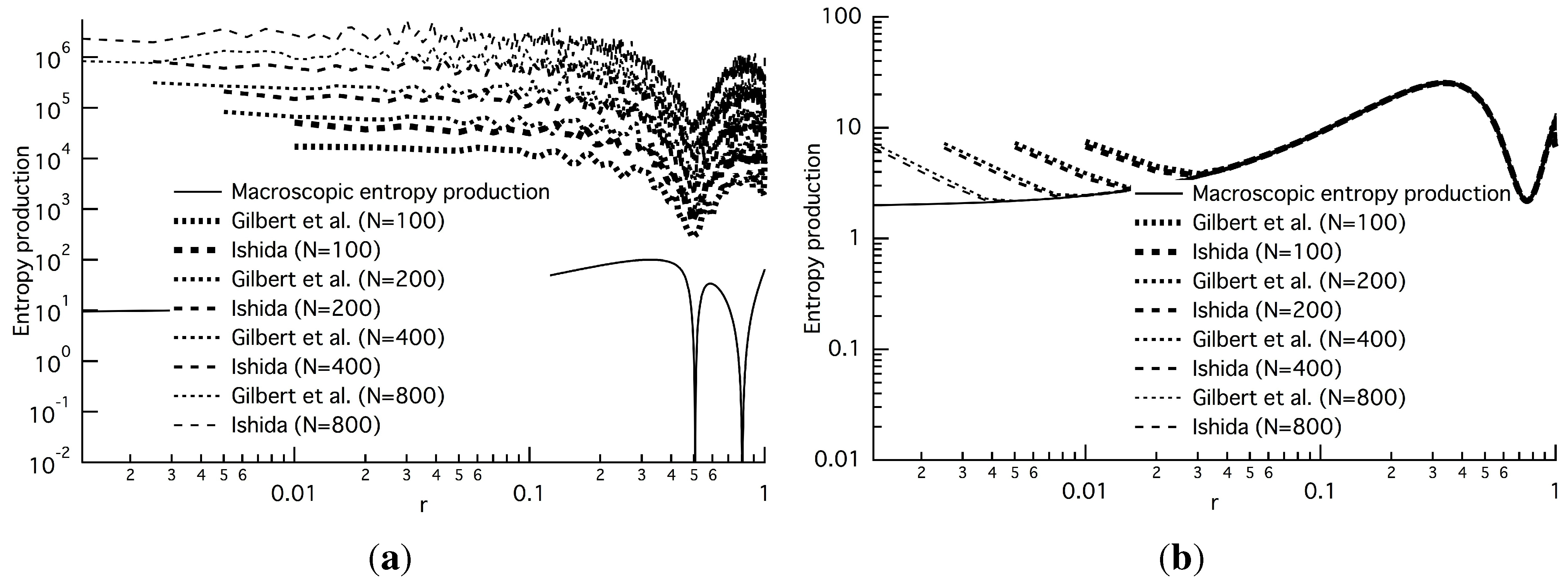
Figure 1 shows the distribution of the macroscopic entropy production, S p , m a c , Equation (45), and the averaged quantities of S p , i ( n ) , Equation (20b), and Δ i S i , Equation (22d), at Pe=1.5. At the initial state, the three quantities do not coincide (Figure 1(a)), because the averaged quantities depend on a sequence of random numbers. After d time steps, however, the dependence vanishes, and we can numerically confirm that the bigger the number of sites N, the more the two averaged quantities will approach the phenomenological expression, S p , m a c , of non-equilibrium thermodynamics (Figure 1(b) and Figure 1(c)), except near both ends. As the transition probability η is uniform for almost all sites in this model, the correspondence between S p , m a c and Δ i S i can be simply regarded as a numerical confirmation of Equation (33c), theoretically proven by Vollmer, Tél and Breymann [6]. As shown in 
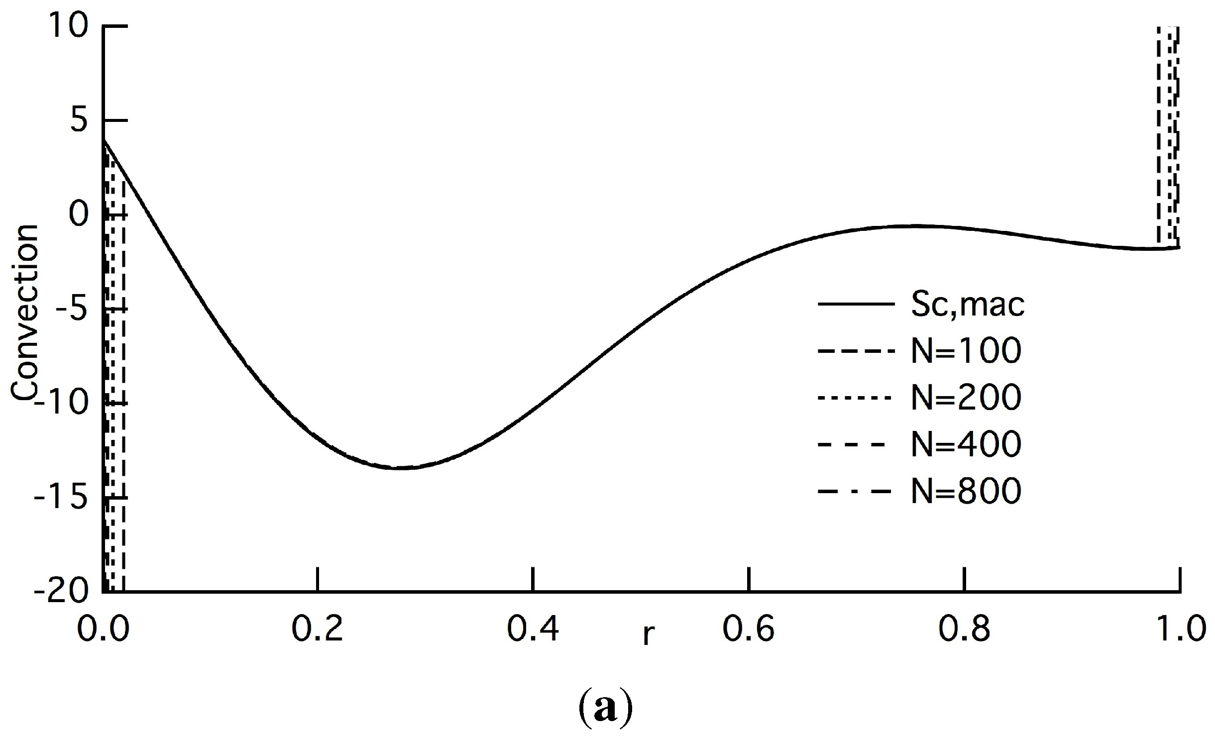
Figure 2, the coincidence in the macroscopic limit is also confirmed for the other terms of the entropy-density balance equation, i.e., S c , m a c , S d , m a c and S t h , m a c , defined in Equation (45). We can also confirm that the averaged quantity of S t h , i ( n ) agrees very well with Φ n ( t h ) , except near the boundaries (Figure 2(c)). We can confirm this coincidence for other Péclet’s numbers. These results also validate the LOE, showing that the major terms in Equations (18) and (20) are averaged to be of O ( 1 ) in the macroscopic limit. In these figures, we can observe that the macroscopic quantities take a local minimum near r = 0.4. This is a result of the initial density profile ρ c , Equation (44), having a local minimum near r = 0.5 and vanishing towards the steady state.
Figure 1. Entropy production at P e = P e ^ = 1.5 , d = 3 and β = 0.5 : (a) t = 0 ; (b) t = λ (Equation (39)); (c) steady state; In this case Ψ 1 , θ 1 , C 1 and q 1 in Equation (44) are 2.4873, 12.733, 3.3487 × 10 2 and zero, respectively. The solid line denotes the macroscopic or phenomenological entropy production, S p , m a c , Equation (45). The dotted and long-dashed lines are the averaged quantities of Δ i S i , Equation (22d), introduced by Gilbert et al. [5], and the entropy production, S p , i ( n ) , Equation (20b), respectively. The two quantities are too close to be distinguished from each other.
Entropy 15 04345 g001aEntropy 15 04345 g001b
Figure 2. Leading terms except the entropy production at t = λ , P e = P e ^ = 1.5 , d = 3 and β = 0.5 : (a) convection; (b) diffusion; (c) entropy flow due to a thermostat. The solid line denotes the macroscopic terms in the macroscopic balance equation for the entropy density, Equation (45): (a) S c , m a c , (b) S d , m a c , (c) S t h , m a c . In Figure 2(a) and 2(b), the other lines denote corresponding averaged terms appearing in Equation (18): (a) S c , i ( n ) , Equation (18b), (b) S d , i ( n ) , Equation (18c). Short-dashed, pecked, long-dashed and dash-dotted lines denote the cases of N=100, 200, 400 and 800, respectively. In Figure 2(c), the dotted and long-dashed lines are Φ n ( t h ) , Equation (34), introduced by Vollmer, Tél and Mátyás [18], and the averaged quantity of entropy flow, S t h , i ( n ) , Equation (20c), respectively. All of the lines agree very well, except near both ends.
Entropy 15 04345 g002aEntropy 15 04345 g002b
Although the details are not given here, we can also numerically confirm Equations (33a) and (33b). Note that the present decomposition makes it possible to directly evaluate all the macroscopic terms in Equation (45) by averaging the corresponding local, coarse-grained terms.
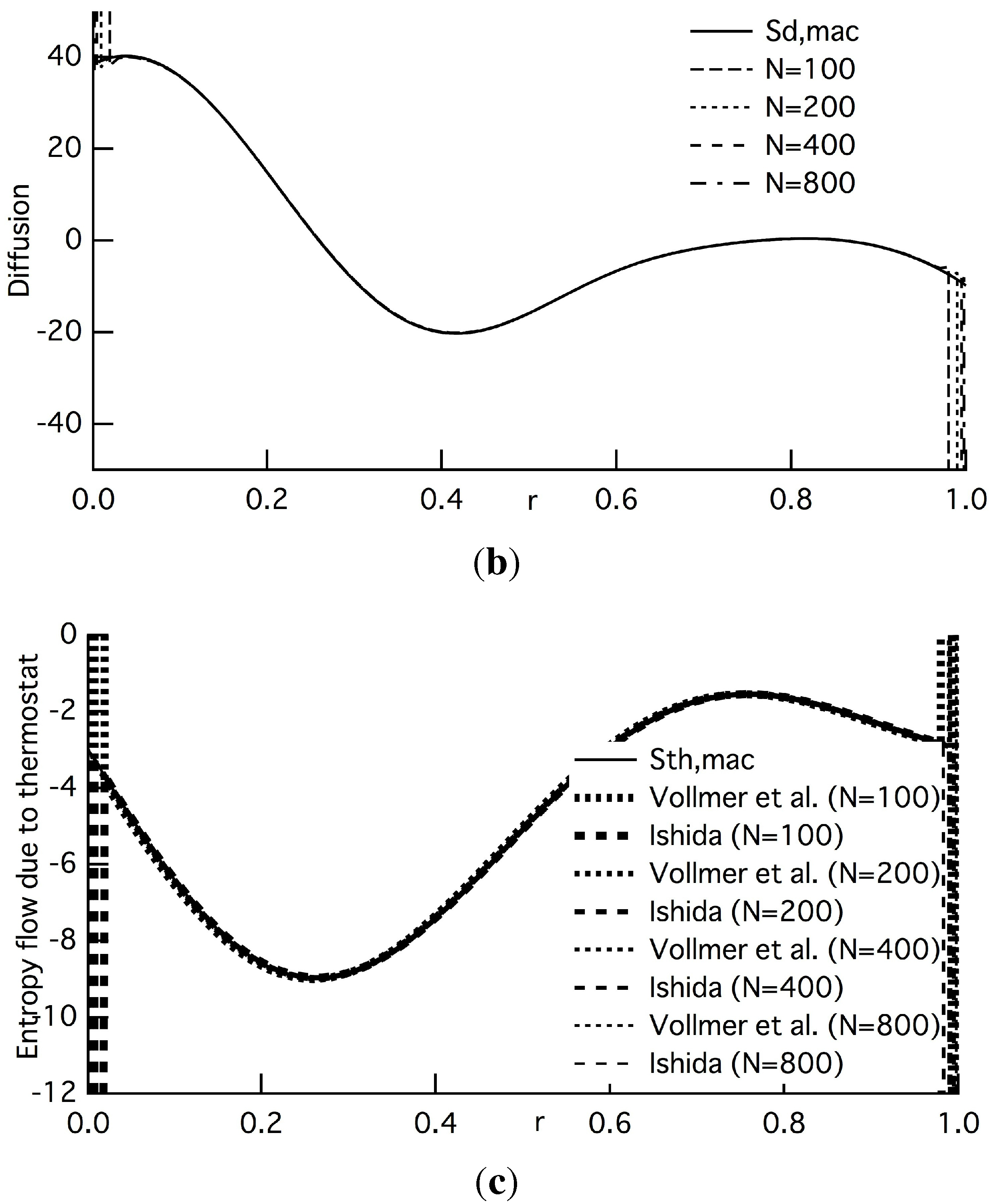
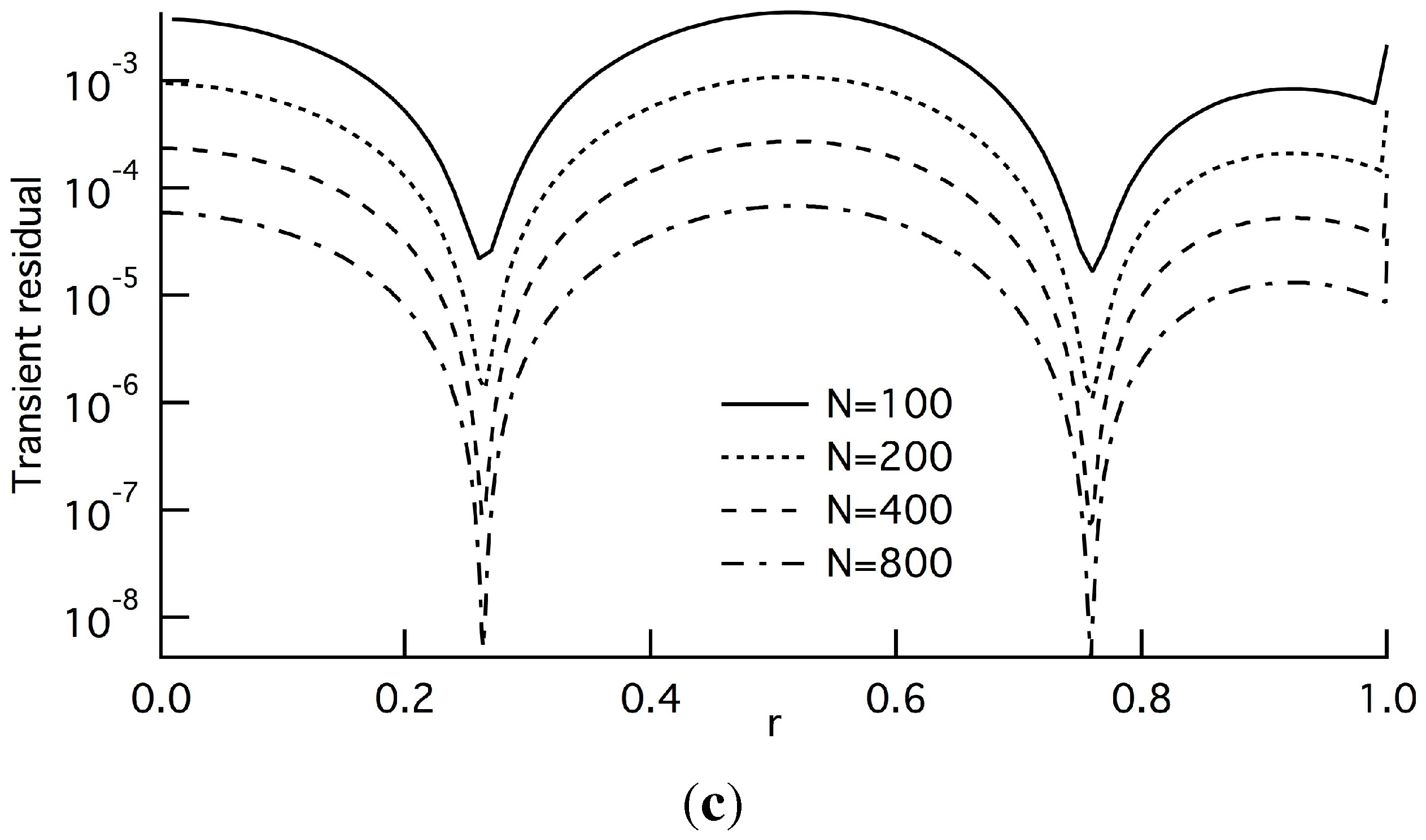
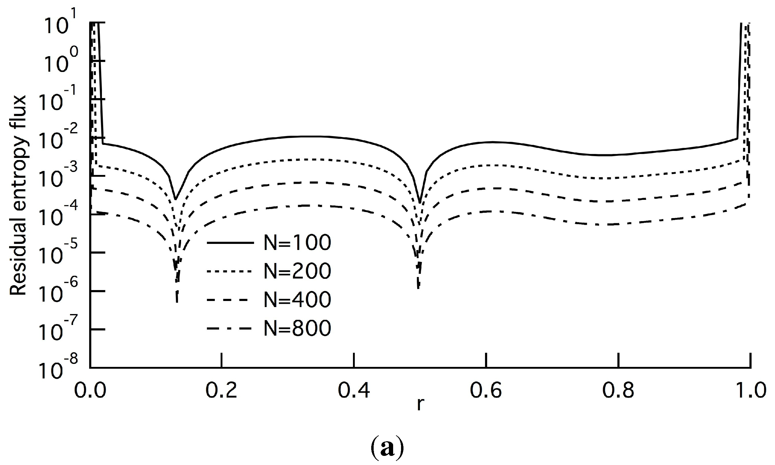
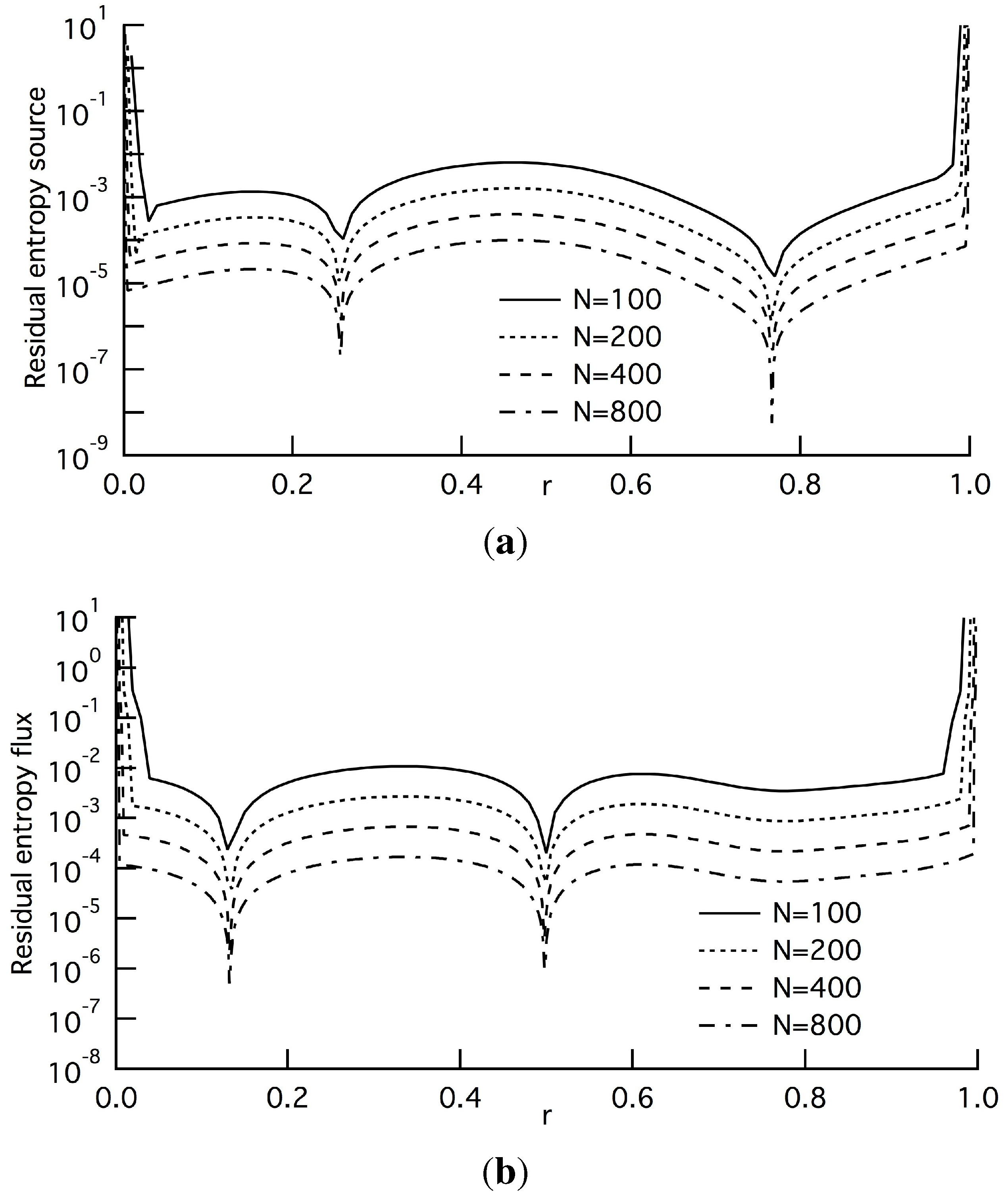
In contrast, as shown in Figures 3(a) and 3(b), the averaged quantities of the residual entropy source and residual entropy flux, r s and r e , are vanishing in the macroscopic limit, and the four lines are equally spaced in the vertical direction for almost all regions of r. This indicates that the two quantities behave according to O ( Δ r b ) as N ( = 1 / Δ r ) increases [10], and b is evaluated to be two from the width in accord with the LOE. This equally-spaced behavior is also confirmed in the averaged quantity of r T (
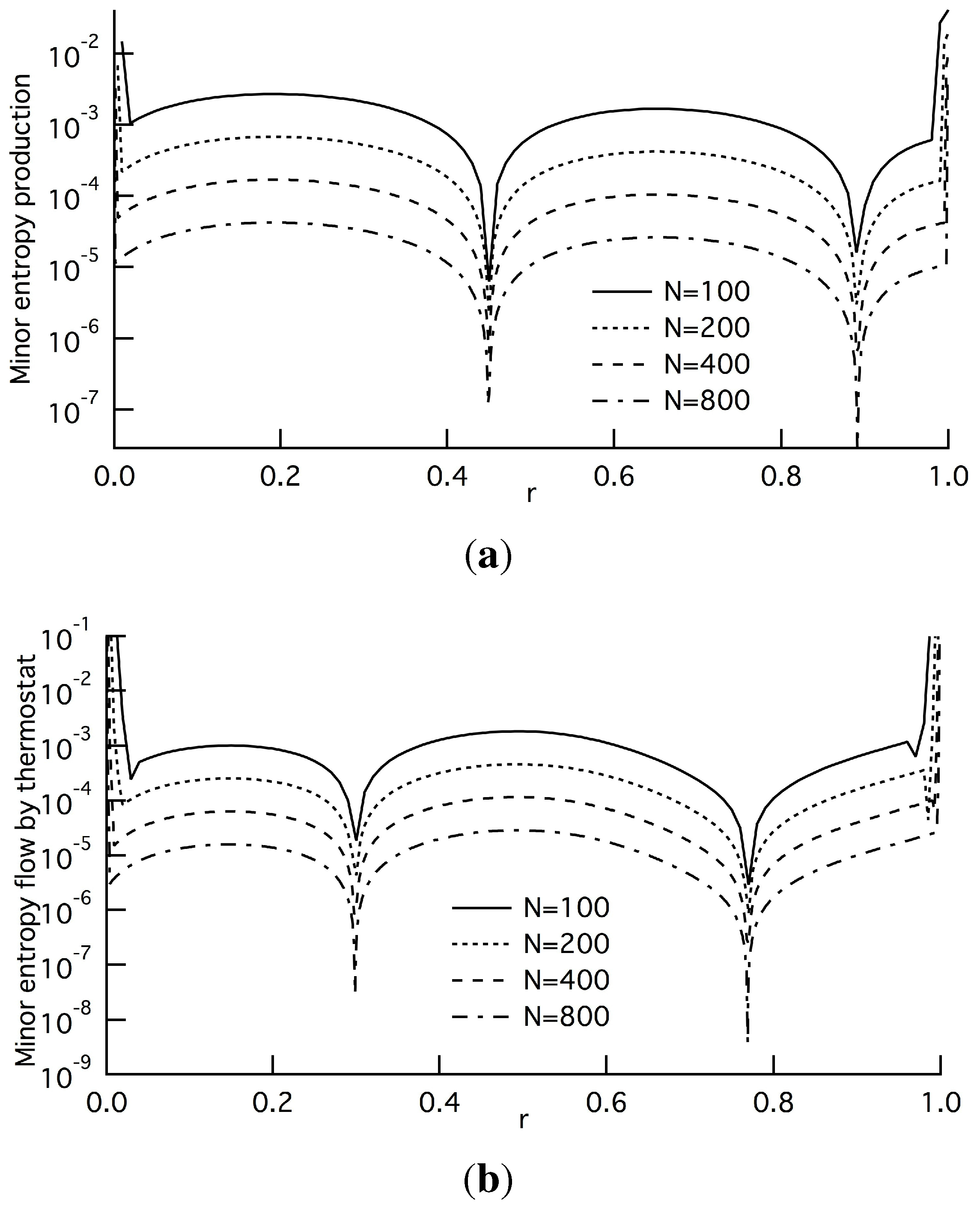
Figure 3(c)) and the two minor terms, r t h and r p (Figure 4). It is surprising that all of the quantities behave according to O ( Δ r 2 ) . As described in Section 3.1, however, the order of the averaged quantity of r T is not of O ( Δ r 2 ) , but of O ( τ ) , and the agreement relies on the present setting of β = 1 / 2 , i.e., τ = O ( Δ r 2 ) . In Figure 3 and Figure 4, we can find several dips, which can be explained by the form of the leading terms of these averaged quantities: the prefactors of Δ r 2 , composed of higher-order derivatives, becomes small at these positions. At this time, however, they are unknown.
In the above-mentioned figures, we find a divergence in the evaluated values near both ends. This indicates that the LOE is not satisfied on the boundary. This is caused by the gap of both the global measure and the transition probability near the boundary site, A N . For the entropy flow due to a thermostat, however, we can interpret the quantities as the heat transfer into the boundary. Table 3 shows such a boundary effect. We can numerically confirm that Φ ( t h ) and Φ ^ ( t h ) agree very well in spite of the disagreement of each component and that they approach the macroscopic entropy flux density, Φ m a c ( t h ) , into the thermostat in the continuous limit. Because of the violation of the LOE at the boundary site, the averaged values of the residual r s and the minor term, r t h , do not vanish in the continuous limit. The effectiveness of the fundamental form S ^ t h , i ( n ) , including the contribution of these terms, therefore, comes from the simplicity of deriving the term only on the basis of the symmetric and antisymmetric properties.
Figure 3. Absolute value of the averaged residual terms at t = λ , P e = P e ^ = 1.5 , d = 3 and β = 0.5 : (a) residual entropy source r s , i ( n ) , Equation (20f); (b) residual entropy flux r e , i ( n ) , Equation (18d); (c) transient residual r T , i ( n ) , Equation (9c). Solid, broken, long-dashed and dash-dotted lines denote the cases of N = 100, 200, 400 and 800, respectively. All of the lines are equally spaced in the vertical direction, and the width indicates that these averaged quantities are of O ( Δ r 2 ) .
Entropy 15 04345 g003aEntropy 15 04345 g003b
Figure 4. Absolute value of the averaged minor terms at t = λ , P e = P e ^ = 1.5 , d = 3 and β = 0.5 : (a) minor entropy production r p , i ( n ) , Equation (20d); (b) minor entropy flow due to a thermostat r t h , i ( n ) , Equation (20e). Solid, broken, long-dashed and dash-dotted lines denote the cases of N = 100, 200, 400 and 800, respectively. All of the lines are also equally spaced in the vertical direction, and the width indicates that these averaged quantities are also of O ( Δ r 2 ) .
Entropy 15 04345 g004
Table 3. Entropy flux density into the boundary ( d = 3 , β = 0.5 ).
Pe Pe ^ Nt Φ ( th ) (Equation (40)) Φ ^ ( th ) (Equation (42)) Φ mac ( th ) (Equation (41))
1.0 × 10 5 1.5100λ 1.94 × 10 2 1.94 × 10 2 1.90 × 10 2
1.0 × 10 5 1.5100 2.92 × 10 2 2.92 × 10 2 2.92 × 10 2
1.51.5100λ 3.90 × 10 2 3.90 × 10 2 3.83 × 10 2
1.51.5800λ 3.07 × 10 3 3.07 × 10 3 3.06 × 10 3
1.51.5100 5.45 × 10 2 5.46 × 10 2 5.40 × 10 2
1.51.5800 4.32 × 10 3 4.32 × 10 3 4.31 × 10 3
1.50.1100λ−20.0−19.8−15.5
1.50.1800λ 1.28 × 10 2 1.28 × 10 2 1.24 × 10 2
101.5100λ 1.36 × 10 3 1.39 × 10 3 1.26 × 10 3
101.5800λ 1.02 × 10 4 1.02 × 10 4 1.01 × 10 4
On the other hand, we can numerically find that the way of partitioning, i.e., β and d, affects the averaged quantity of the residual and minor terms. 
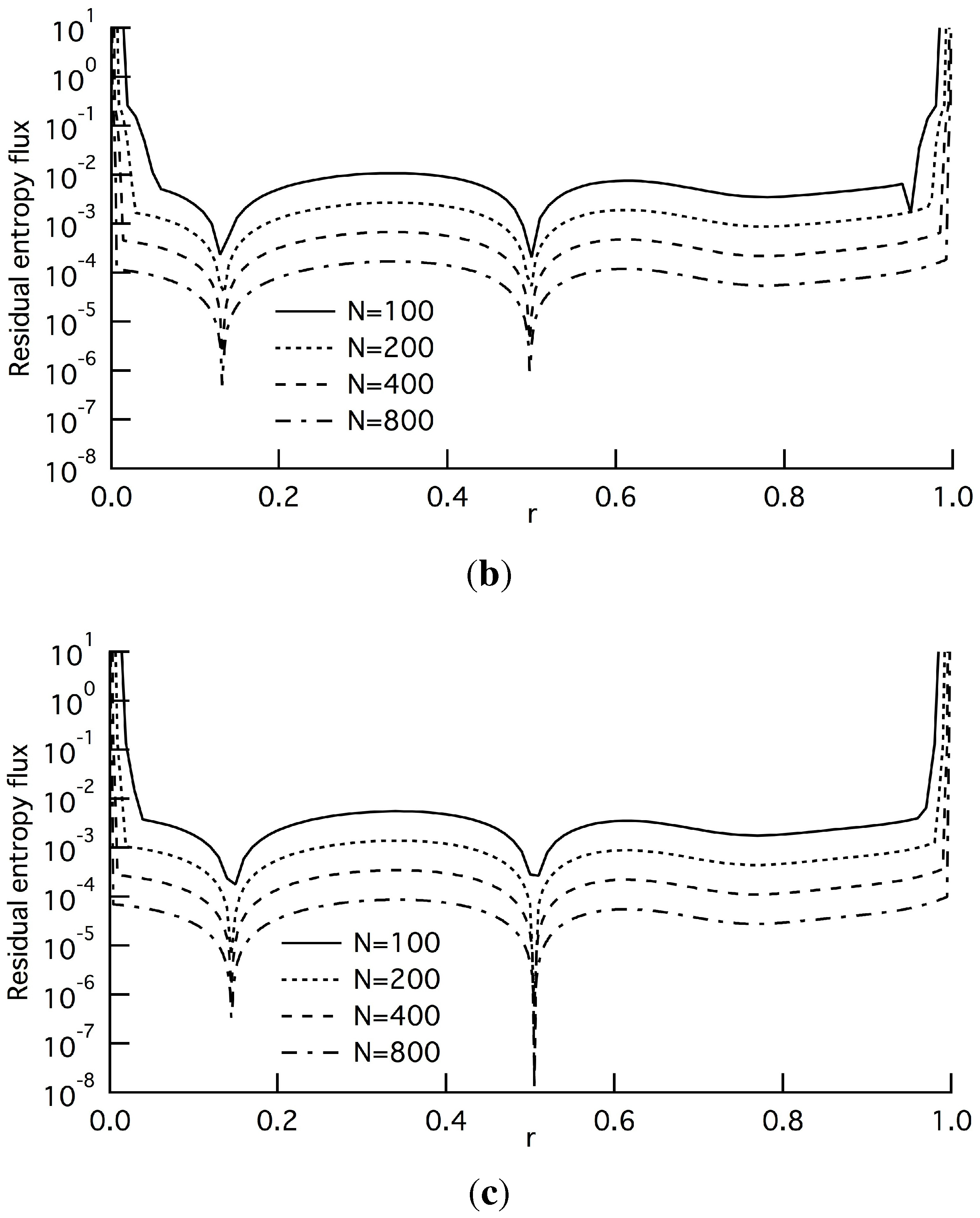
Figure 5 shows the distributions of the averaged residual entropy flux when β and d are changed at t = λ and Pe = 1.5. We can ascertain that the partitioning does affect the quantity. However, the four lines are equally spaced, and the width is identical. That is to say, the order of O ( Δ r 2 ) of the averaged residual, estimated from the LOE, is independent of the partitioning. This is the case for the other residual and minor terms, too.
Figure 5. Partitioning effects on the absolute value of averaged residual entropy flux r e , i ( n ) , Equation (18d), at t = λ , P e = P e ^ = 1.5 : (a) d = 1 , β = 0.5 ; (b) d = 5 , β = 0.5 ; (c) d = 3 , β = 0.25 . Solid, broken, long-dashed and dash-dotted lines denote the cases of N=100, 200, 400 and 800, respectively. The partitioning effects appear. However, all of the lines are equally spaced in the vertical direction, and the width, i.e., the order of these quantities of O ( Δ r 2 ) , is independent of the partitioning.
Entropy 15 04345 g005aEntropy 15 04345 g005b
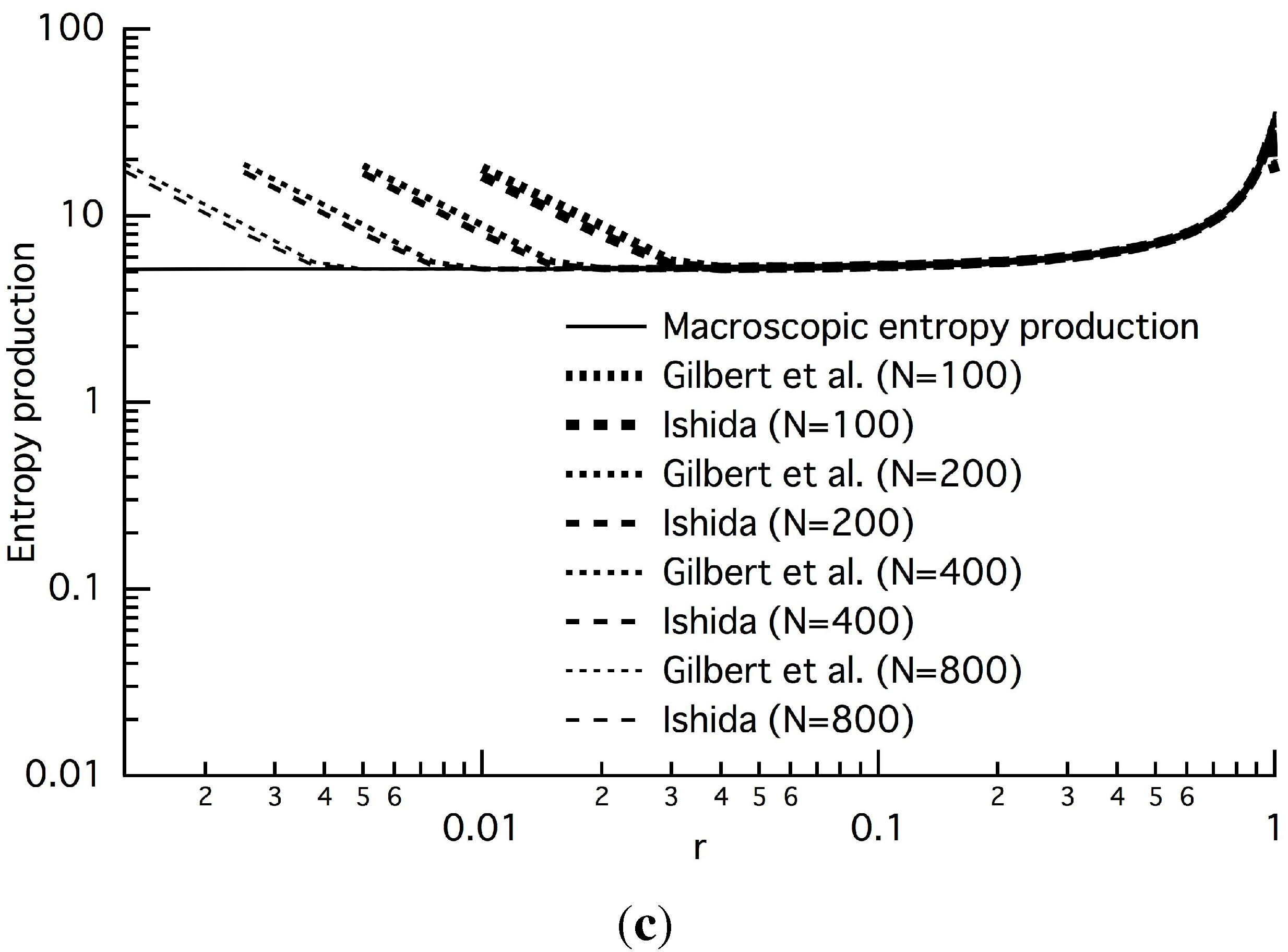
Similarly, the averaged quantities of the leading terms, i.e., the zeroth-order (O(1)) terms, are quantitatively affected by higher order terms. Figure 6 shows the averaged entropy production at Pe = 1.5. As shown in the figure, the way of partitioning affects the quantity while N is relatively small. However, we can confirm that the quantity comes to be independent of the partitioning when N is sufficiently large. This indicates that the limiting value as N , as well as the order of O ( Δ r 0 ) estimated from the law are also independent of the partitioning.
The fact that the averaged quantities and their orders are independent of the resolution parameter d are consistent with the discussions by Gaspard, Gilbert and Barra et al. [5,11,12,13,14,15,16,17,21]. At the same time, we now confirm that the coarsest partitioning of d=1 is fine enough to recover macroscopic quantities. This is in accordance with the discussion about “structural stability” by Vollmer, Breymann and Mátyás et al. [6,7,20]. Since the inverse mapping of a partition of d=1 (level-1 partition) is a full site (level-0 partition), we cannot treat the past density distribution on a site. Thus, in order to recover the results of thermodynamics, it is sufficient for us to consider one-time mapping from an initial uniform density [6,7,8,9,18,19,20,22].
These properties are essential for the coarse-grained statistics [7,13]. However, the partitioning can affect averaged quantities not discussed in this study. This is an issue for us to deal with in the future.
Figure 6. Partitioning effects on the entropy production at t = λ , P e = P e ^ = 1.5 : (a) d = 1 , β = 0.5 ; (b) d = 5 , β = 0.5 ; (c) d = 3 , β = 0.25 . The solid line denotes the macroscopic entropy production S p , m a c , Equation (45). The dotted and long-dashed lines are the averaged quantities of Δ i S i , Equation (22d), and the entropy production S p , i ( n ) , Equation (20b), respectively. The two averaged quantities are too close to be distinguished from each other. The partitioning effects are also confirmed. As the site number N increases, however, the effects are weakened.
Entropy 15 04345 g006

4. Concluding Remarks

On the basis of the symmetric properties for the inversion of the partition, the density pairs and a given drift velocity, the equation for local entropy density is decomposed to evaluate the unsteady macroscopic terms in a phenomenological entropy-density balance equation for the system driven by a thermostat. This is done by the decomposition of the time-evolution operator for the local entropy density on the level of a master equation. In addition, a law of order estimation (LOE) is introduced to explain the behavior of averaged quantities in the macroscopic limit. The law is empirically derived from the numerical results for the case of the partitioning parameters, β and d, the diffusion coefficient, D, and the drift velocity, v, being constant in the bulk system, as discussed in this and previous studies (Ishida [10]). Their validity and applicability are numerically confirmed on a dissipative and invertible multibaker chain system, called a circuit model. The main results are as follows:
(1) On the basis of the symmetric and antisymmetric properties for the inversion of the partition, the density pairs and a given drift velocity, the equation for local entropy density is decomposed into an unsteady term and leading terms describing convection, diffusion, entropy flow due to a thermostat and entropy production. The averaged quantity of each term agrees with a corresponding macroscopic term of irreversible thermodynamics in the macroscopic limit. The LOE can explain the convergent behavior in the bulk system. The decomposition can be utilized even for the evaluation of the entropy flux density into the thermostat at the boundary and is expected to be applicable to many systems.
(2) The entropy production term can be further decomposed into nonnegative, minor and residual terms. The minor term vanishes in volume-preserving systems. The behavior of the averaged residual term, which vanishes in the macroscopic limit, is also explained by the estimation law. The law is responsible for the positive entropy production in volume-preserving systems far from equilibrium. On the other hand, the vanishing behavior of the minor term, confirmed numerically, is responsible for the positivity in thermostated systems far from steady state.
(3) The way of partitioning, i.e., setting the value of β and d, affects the averaged quantity of higher order terms ( O ( Δ r a ) , a > 0 ). However, the order, a, itself, estimated by the LOE, is independent of the partitioning. Similarly, the averaged quantities of leading terms, i.e., the zeroth-order (O(1)) terms, are quantitatively affected by the higher order terms and depend on the partitioning when the site number N ( = 1 / Δ r ) is finite. However, the effect vanishes in the macroscopic limit, N . Therefore, its limiting value, as well as the order one estimated from the law, are also independent of the partitioning.

Acknowledgments

I am grateful to Joel L. Lebowitz and Sheldon Goldstein for enlightening discussions. This work was partially supported by the Japan Society for the Promotion of Science, the Institutional Program “Development of International Network for Training of Young Researchers Exploring Multidisciplinary Fields”, No. J091113016.

Conflicts of Interest

The author declares no conflict of interest.

References

  1. Ruelle, D. Positivity of entropy production in nonequilibrium statistical mechanics. J. Stat. Phys. 1996, 85, 1–23. [Google Scholar] [CrossRef]
  2. Chernov, N.L.; Lebowitz, J.L. Stationary shear flow in boundary driven Hamiltonian systems. Phys. Rev. Lett. 1995, 75, 2831–2834. [Google Scholar] [CrossRef] [PubMed]
  3. Chernov, N.I.; Lebowitz, J.L. Stationary nonequilibrium states in boundary-driven Hamiltonia systems: Shear flow. J. Stat. Phys. 1997, 86, 953–990. [Google Scholar] [CrossRef]
  4. Barra, F.; Gilbert, T.; Reyes, S. Conductivity of the self-similar Lorentz channel. Int. J. Bifur. Chaos 2000, 19, 2687–2694. [Google Scholar] [CrossRef]
  5. Gilbert, T.; Dorfman, J.R. Entropy production: From open volume-preserving to dissipative system. J. Stat. Phys. 1999, 96, 225–269. [Google Scholar] [CrossRef]
  6. Vollmer, J.; Tél, T.; Breymann, W. Entropy balance in the presence of drift and diffusion currents: An elementary chaotic map approach. Phys. Rev. E 1998, 58, 1672–1684. [Google Scholar] [CrossRef]
  7. Breymann, W.; Tél, T.; Vollmer, J. Entropy balance, time reversibility, and mass transport in dyamical systems. Chaos 1998, 8, 396–408. [Google Scholar] [CrossRef] [PubMed]
  8. Vollmer, J.; Tél, T.; Breymann, W. Equivalence of irreversible entropy production in driven systems: An elementary chaotic map approach. Phys. Rev. Lett. 1997, 79, 2759–2762. [Google Scholar] [CrossRef]
  9. Tél, T.; Vollmer, J.; Breymann, W. Transient chaos: The origin of transport in driven systems. Europhys. Lett. 1996, 35, 659–664. [Google Scholar] [CrossRef]
  10. Ishida, H. A decomposed equation for local entropy and entropy production in volume-preserving coarse-grained systems. Physica A 2009, 388, 332–342. [Google Scholar] [CrossRef]
  11. Tasaki, S.; Gaspard, P. Fick’s law and fractality of nonequilibrium stationary states in a reversible multibaker map. J. Stat. Phys. 1995, 81, 935–987. [Google Scholar] [CrossRef]
  12. Gilbert, T.; Dorfman, J.R. Entropy production in a persistent random walk. Physica A 2000, 282, 427–449. [Google Scholar] [CrossRef]
  13. Gilbert, T.; Dorfman, J.R.; Gaspard, P. Entropy production, fractals, and relaxation to equilibrium. Phys. Rev. Lett. 2000, 85, 1606–1609. [Google Scholar] [CrossRef] [PubMed]
  14. Gaspard, P. Entropy production in open volume-preserving systems. J. Stat. Phys. 1997, 88, 1215–1240. [Google Scholar] [CrossRef]
  15. Dorfman, J.R.; Gaspard, P.; Gilbert, T. Entropy production of diffusion in spatially periodic deterministic systems. Phys. Rev. E 2002, 66, 026110. [Google Scholar] [CrossRef] [PubMed]
  16. Barra, F.; Gaspard, P.; Gilbert, T. Fractality of the nonequilibrium stationary states of open volume-preserving systems. I. tagged particle diffusion. Phys. Rev. E 2009, 80, 021126. [Google Scholar] [CrossRef] [PubMed]
  17. Barra, F.; Gaspard, P.; Gilbert, T. Fractality of the nonequilibrium stationary states of open volume-preserving systems. II. Galton boards. Phys. Rev. E 2009, 80, 021126. [Google Scholar] [CrossRef] [PubMed]
  18. Vollmer, J.; Tél, T.; Mátyás, L. Modeling thermostating, entropy currents, and cross effects by dynamical system. J. Stat. Phys. 2000, 101, 79–105. [Google Scholar] [CrossRef]
  19. Mátyás, L.; Tél, T.; Vollmer, J. Thermodynamic cross effects from dynamical systems. Phys. Rev. E 2000, 61, R3295–R3298. [Google Scholar] [CrossRef]
  20. Mátyás, L.; Tél, T.; Vollmer, J. Multibaker map for thermodynamic cross effects in dynamical systems. Phys. Rev. E 2000, 62, 349–365. [Google Scholar] [CrossRef]
  21. Gaspard, P. Chaos, Scattering and Statistical Mechanics; Cambridge University Press: New York, NY, USA, 1998. [Google Scholar]
  22. Vollmer, J. Chaos, spatial extension, transport, and non-equilibrium thermodynamics. Phys. Rep. 2002, 372, 131–267. [Google Scholar] [CrossRef]
  23. Schnakenberg, J. Network theory of microscopic and macroscopic behavior of master equation systems. Rev. Mod. Phys. 1976, 48, 571–585. [Google Scholar] [CrossRef]
  24. Dorfman, J.R. An Introduction to Chaos in Nonequilibrium Statistical Mechanics; Cambridge University Press: Cambridge, UK, 1999. [Google Scholar]
  25. Patankar, S.V. Numerical Heat Transfer and Fluid Flow; Hemisphere Publishing Co.: New York, NY, USA, 1980. [Google Scholar]
  26. Fushimi, M. Random number generation with the recursion Xt = Xt−3pXt-3q. J. Comput. Appl. Math. 1990, 31, 105–118. [Google Scholar] [CrossRef]

