Non-Equilibrium Statistical Mechanics Inspired by Modern Information Theory

Abstract

A collection of recent papers revisit how to quantify the relationship between information and work in the light of modern information theory, so-called single-shot information theory. This is an introduction to those papers, from the perspective of the author. Many of the results may be viewed as a quantification of how much work a generalized Maxwell’s daemon can extract as a function of its extra information. These expressions do not in general involve the Shannon/von Neumann entropy but rather quantities from single-shot information theory. In a limit of large systems composed of many identical and independent parts the Shannon/von Neumann entropy is recovered.

1. Introduction

This is an introduction to a new approach to statistical mechanics, which may be called single-shot statistical mechanics [1,2,3,4,5,6]. There are certain obstacles to people working on this approach: motivational (why is it worth the effort?), technical (the papers to date are often quite mathematical, involving novel information theory techniques) and conceptual (what is the role of information entropy in statistical mechanics, what is work?). With this in mind, we try to remove these hurdles. We imagine the reader as someone who is considering doing research on this topic.

What do we do?—We calculate expressions for how much work one can extract in the context of a system, called the working medium, undergoing a transform of its state and Hamiltonian. You may think of the work as energy transferred to another system, the work reservoir, during the transform of the working medium system. We are in particular interested in deriving expressions for the optimal work given the initial and final conditions. This means the largest increase in the work reservoir we can attain or, in the case where work needs to be put in, the lowest decrease we can attain. We also consider cycles of such processes, like heat engines, as well as quantitative restrictions on how a system can change when it interacts with a heat-bath. We try to make as general statements as possible, assuming as little as possible about the initial and final conditions, and are now at a stage where neither the initial nor final state needs to be a thermal state and the initial and final Hamiltonians can be arbitrary. Accordingly, we can answer how much work a Maxwell’s daemon [7] type agent with insider information beyond that of the standard thermodynamical observer can extract from a system, as a function of its extra information. We can address that question because the information the agent has would be encoded in and thus represented by the state it assigns to the system. We also consider daemons with a quantum memory. In this case it is not the state of the system that represents the knowledge, as this is not well-defined, but rather the correlations in the joint system-memory system.

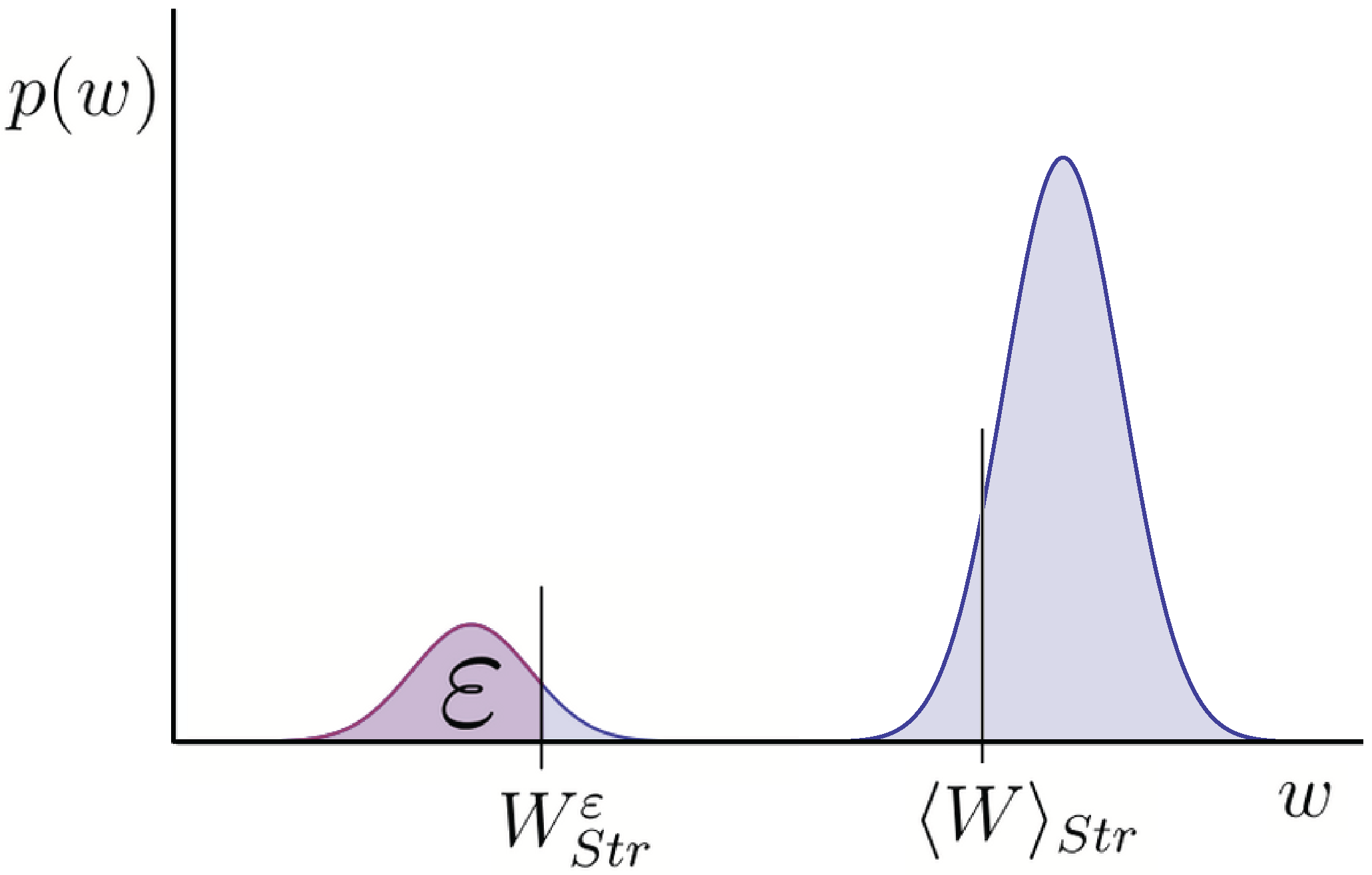
We depart from standard thermodynamics in several ways. Dropping the assumption of thermal states, as already mentioned, is one of them. We also depart by being interested not in the average work $\langle W\rangle$ but in the work that can be guaranteed in any single realization, up to failure probability ε, $W^{\epsilon }$, see Figure 1. In the limiting cases where the probability distribution over work for a given protocol/strategy $Str.$ is a delta-function on some value it does not matter which quantity one uses, as in that case ${\langle W\rangle }_{Str}=W_{Str}^{\epsilon }\forall \epsilon \in (0,1]$. But when there is a significant spread the two quantities can differ greatly.

Figure 1. Example of a distribution $p\left(w\right)$ over energy w transferred to work-reservoir using some strategy $Str$. The distribution in this instance has two peaks. ${\langle W\rangle }_{Str}$ is the average of this distribution. $W_{Str}^{\epsilon }$ is the guaranteed work up to failure probability ε. ε is the probability of getting less work than $W_{Str}^{\epsilon }$. When distributions have a significant spread around the average, as is the case here, these two quantities can differ greatly. We argue $W_{Str}^{\epsilon }$ is a more useful quantity to know.

Figure 1. Example of a distribution $p\left(w\right)$ over energy w transferred to work-reservoir using some strategy $Str$. The distribution in this instance has two peaks. ${\langle W\rangle }_{Str}$ is the average of this distribution. $W_{Str}^{\epsilon }$ is the guaranteed work up to failure probability ε. ε is the probability of getting less work than $W_{Str}^{\epsilon }$. When distributions have a significant spread around the average, as is the case here, these two quantities can differ greatly. We argue $W_{Str}^{\epsilon }$ is a more useful quantity to know.

Why?—Let me begin with the motivation for considering the guaranteed work rather than the average. Suppose I apply for a job to lift boxes from the floor onto the table. The potential energy gain of the box, $mgh$ is the energy transferred to the work reservoir, assuming there is no additional kinetic energy. Now consider two different approaches I may use to lift the box: (I) I lift it in the natural way from the floor, just high enough so that it sits atop the table, succeeding say $99\%$ of the time; ($II$) I throw the box high in the air up to a higher shelf, succeeding say $1\%$ of the time, and otherwise crashing to the floor. Now actually these two approaches will, by a suitable choice of height of the table and shelf, give the same $\langle mgh\rangle$. I would suggest, however, that you would not find me a very useful lifter if I insist on using approach $II$. If, instead of using $\langle mgh\rangle$ as the measure of work, you used $W^{\epsilon }$, you could see that for example $W_I^{0.009}=mgh$ and $W_{II}^{0.009}=0$: the second approach suddenly looks very bad. This suggests that when there are significant fluctuations in the work output, the guaranteed work is more useful to know than the average work. In many physical scenarios, very small systems in particular, fluctuations of this type are indeed significant. Moreover thresholds like the table in the above example do appear frequently in nature, for example as activation energies and semi-conductor band-gaps. Distinguishing between guaranteed and average work in these systems is crucial.

Another key motivation for this research direction was, and remains, the success of single-shot information theory in the context of quantum cryptography and quantum information more generally. (I will introduce this approach later in this note). As there is a history of fruitful interchange of ideas between information theory and statistical mechanics (for example Jayne’s approach to thermodynamics was heavily inspired by information theory and the von Neumann entropy emerged from thermodynamic considerations) we wondered whether this new approach to information theory can be useful in statistical mechanics, and whether information theory can even get something back. As a starting point we wanted a place where entropy plays a concrete role in statistical mechanics, and work extraction scenarios are both very concrete and important.

There are other important reasons to be interested in the relation between work and entropy. From the perspective of intellectual curiosity, there is an intriguing tension between the subjectivity of entropy (if I flip a coin and look at it, but do not show you, the coin has entropy 1 according to you but 0 according to me), and the apparent objectivity of, say, a weight being lifted by a certain amount. How can these appear in the same equation as is often the case in thermodynamics? I will answer this question later in this note.

There is also a more directly practical motivation. One of mankind’s greatest technological problems is the heating of microelectronic components, as for example the heating of the laptop I am using to write this. The power densities of typical micro-electronic circuits are approaching those of a light-bulb filament [8]. Further miniaturization and energy efficiency both seem to demand novel, and probably disruptive, technologies which do not generate so much heat. Existing results by Bennett and Landauer on the fundamental limits to the energy consumption of computers help to guide the debate concerning what is possible here [8,9], and we may hope to contribute similarly.

Quantum information concepts and techniques can contribute to this type of research as we have extensively thought about entropy and how to quantify it.

A disclaimer: this brief note does not contain all the results in the papers mentioned. It is written from my perspective. It should in particular be noted that whilst I will here use the language of work extraction games [4] in particular uses the so-called resource theory paradigm. Moreover this is not a review of the wide field of quantum/nano/non-equilibrium thermodynamics. For other interesting results and approaches see for example [10,11,12,13,14,15,16,17] to mention but a few.

The outline is as follows: Firstly we define and briefly explain single-shot entropies. Then we consider work extraction games and expressions for optimality in them.

2. Single-Shot Entropies (a.k.a Smooth Entropies)

We now introduce single-shot information theory, to a large extent pioneered in [18]. It is centred around the min and max entropies.

2.1. Min and Max Entropies

Let us begin with the classical case as there is a straightforward way to go the quantum case from there.

An entropy measure is, loosely speaking, a functional that takes a probability distribution as an input and outputs a real number that is supposed to say something about how random the distribution is, or in other words, how big our ignorance is about the value of the random variable in question.

In information theory one tends to demand that the entropy measure has some specific operational importance, like $S\left(\overrightarrow{p}\right)$, where $\overrightarrow{p}$ is a probability distribution over messages, should tell us the size -in number of bits- of a memory that is necessary and sufficient to assign a unique state in the memory to each message. In other words, what is the most compressed memory size, in number of bits, that suffices to store or carry a message from this distribution. Let us consider what S would then be.

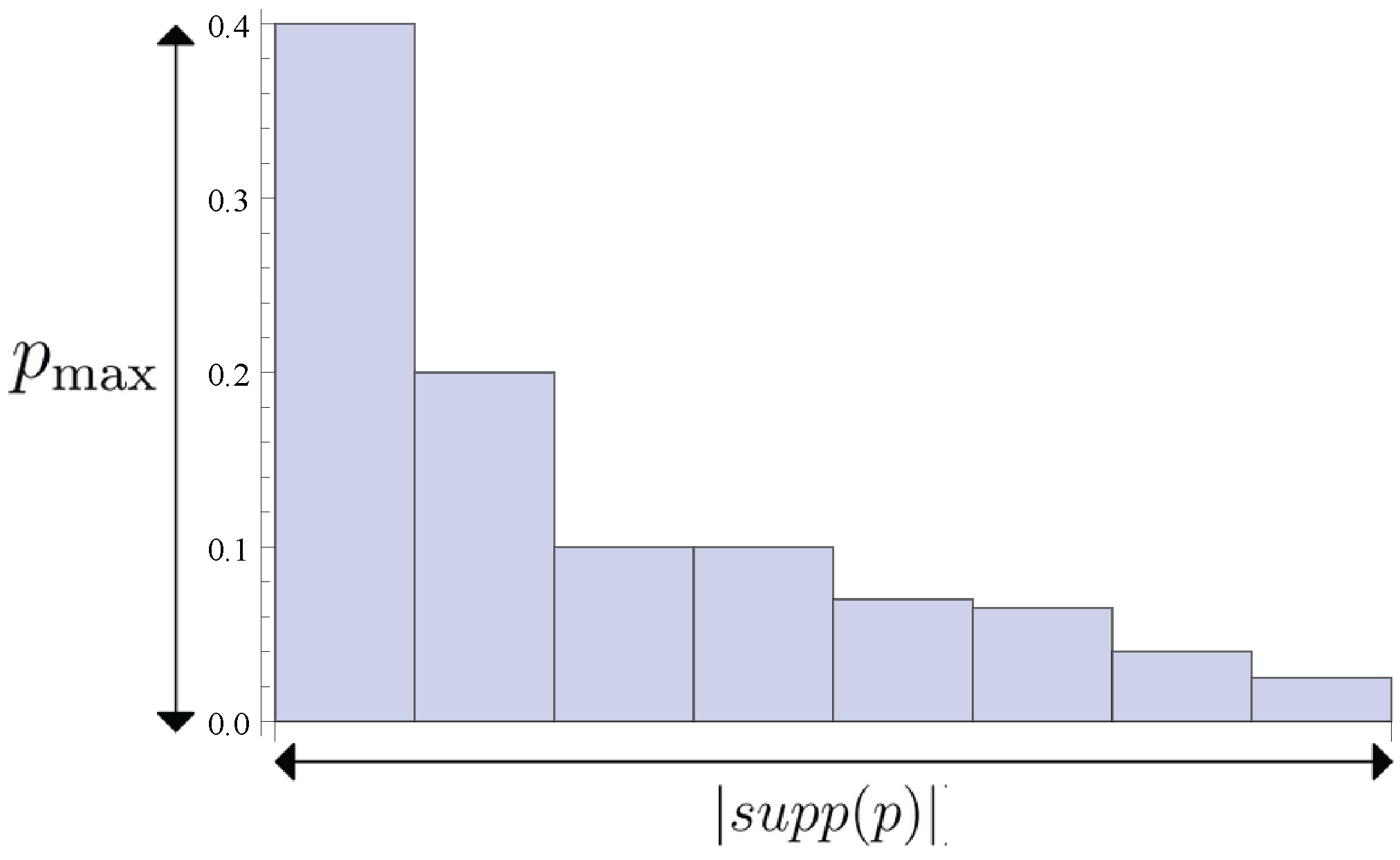
For the example of the distribution in Figure 2 our memory needs to have 8 states, meaning ${log}_2\left(8\right)=3$ bits. We see that more generally $S={log}_2(|supp\left(\overrightarrow{p}\right)|)$. (Strictly speaking the memory size in bits is in general the nearest upper integer, $\lceil S\rceil$). This entropy frequently appears in single-shot information theory, it is called $S_{max}$ because it turns out to be an upper bound to many other entropies, including the well-known Shannon entropy $S=-{\sum }_i{p}_i{log}_2{p}_i$.

Figure 2. This depicts a probability distribution with support on 8 events and event 1 having the highest probability of occurring (with $p_{max}=0.4$). These two numbers are crucial aspects of a distribution more generally. Its support size may be called its width and the max probability its height. For some operational questions one matters and for some the other. The Shannon entropy cares about both, but the min entropy only cares about the height and the max entropy only cares about the width.

Figure 2. This depicts a probability distribution with support on 8 events and event 1 having the highest probability of occurring (with $p_{max}=0.4$). These two numbers are crucial aspects of a distribution more generally. Its support size may be called its width and the max probability its height. For some operational questions one matters and for some the other. The Shannon entropy cares about both, but the min entropy only cares about the height and the max entropy only cares about the width.

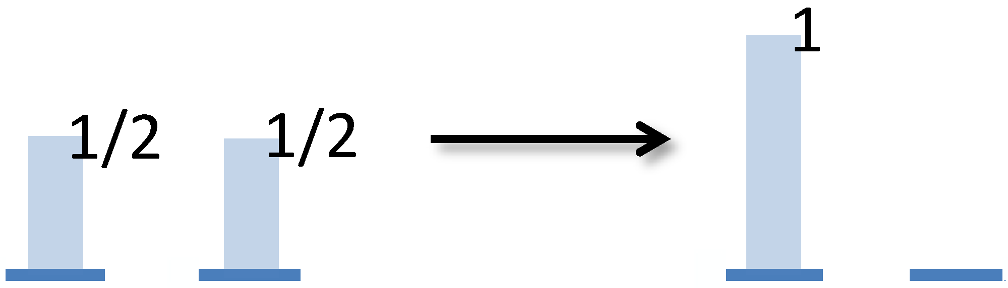
Asking a different operational question can lead to a different entropy measure. Suppose you are given n bits and some probability distribution over their states. What you really want is a set of uniformly random bits though. Maybe you run a casino and people will bet on the state. You would like to extract uniform randomness from this distribution with as a large support as possible. As a concrete example you can consider a roulette-wheel where some of the slots have an especially low probability of getting occupied. One thing one could do is to group several slots together, labeling them as one slot. The probability of that slot being occupied is then the sum of the probabilities of the individual slots. Or one may have two bits and be allowed to choose to use only one of them, s.t. $\left[p\right(00),p(01),p(10),p(11\left)\right]$ becomes $\left[p\right(00)+p(01),p(10)+p(11\left)\right]$. More generally one may allow any such grouping of events: this could also be called a coarse-graining. If we are lucky this grouping can yield a uniform distribution with height $p_{max}$ and width $1/p_{max}$, where $p_{max}$ is the maximum probability of the initial distribution. However we cannot have a greater width, because this procedure, which only adds probabilities, cannot decrease $p_{max}$. Thus the width of any uniform distribution obtained from this grouping is at most $1/p_{max}$, and the maximum number of uniformly random bits is at most $log(1/p_{max})$. One defines $S_{min}:=log(1/p_{max})$.

In summary:

$$S_{max}:={log}_2(|supp\left(p\right)|)$$

(1)

$$S_{min}:={log}_2\left(\frac{1}{p_{max}}\right)$$

(2)

and

$$S:=\sum _i{p}_i{log}_2\left(\frac{1}{p_i}\right)$$

(3)

The definitions for the quantum case are recovered simply by replacing $p_i$ with ${\lambda }_i$, the eigenvalues of the density matrix.

Readers interested in Renyi entropies $S_{\alpha }:=(log{\sum }_i{p}_i^{\alpha })/(1-\alpha )$ may note that $S_{max}=S_0,S_{min}=S_{\infty }$ and $S=S_1$ as can be seen by taking the limit as $\alpha \to 1$ and using L’Hôpital’s rule. (A small note of caution is that sometimes people refer to the min entropy as $S_2$ and the max entropy as $S_{1/2}$. There are reasons for why sometimes this is preferable, but we do not need to use those entropies here; here we consistently refer to $S_0$ as the max entropy and $S_{\infty }$ as the min entropy). Moreover it is useful, partly just to remember the naming convention(!), that $S_{min}\le S_{\alpha }\le S_{max}\forall \alpha$ and in particular

$$S_{min}\le S\le S_{max}$$

(4)

2.2. Smoothing

The min and max entropies defined above are the two crucial entropies in single-shot information theory. In standard Shannon information theory there is only one entropy, the Shannon entropy. The min and max entropy will actually, as will be described later, converge to the Shannon entropy in a particular way for certain states. Only for those states does the Shannon entropy have the desired operational meaning for information compression and randomness extraction. Reaching this limit involves firstly doing something to the entropy called, for historical reasons, smoothing.

The definition of the smooth max entropy is

$$S_{max}^{\epsilon }\left(\rho \right):=min{S}_{max}\left({\rho }^{\prime }\right)|d(\rho ,{\rho }^{\prime })\le \epsilon$$

(5)

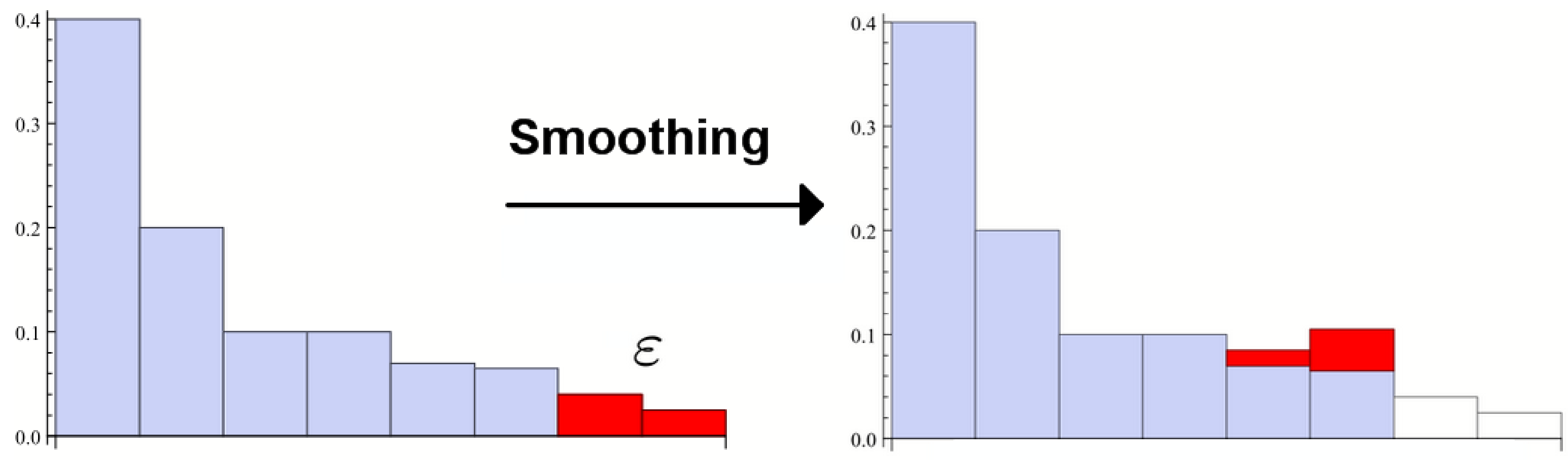
where ρ and ${\rho }^{\prime }$ are density matrices and $d(·,·)$ is a distance measure. If d is the trace distance the smoothing looks like in Figure 3.

Figure 3. Smoothing the max entropy amounts to taking the lowest probabilities of the distribution away, up until the point that their weights sum to ε, and then taking the max entropy of that new distribution. If there are many events with small probabilities the smooth entropy can thus be much lower than the non-smooth one.

Figure 3. Smoothing the max entropy amounts to taking the lowest probabilities of the distribution away, up until the point that their weights sum to ε, and then taking the max entropy of that new distribution. If there are many events with small probabilities the smooth entropy can thus be much lower than the non-smooth one.

A good interpretation is that the smooth entropy is effectively $S_{max}^{\epsilon }\left(\rho \right)$, so that the necessary memory-size for example is effectively given by the smooth entropy. ε then quantifies what error probability one tolerates.

One reason smoothing is important is that

$$lim(n\to \infty ,\epsilon \to 0)\frac{S_{max}^{\epsilon }\left({\rho }^{\otimes n}\right)}{n}=S\left(\rho \right)$$

(6)

This limit is called the asymptotic i.i.d. regime, or the von Neumann regime (recall that i.i.d. means independently, identically distributed, so that an i.i.d. state with n samples associated with state ρ is ${\rho }^{\otimes n}$). The same statement holds for the smooth min entropy, which is defined as

$$S_{min}^{\epsilon }\left(\rho \right):=max{S}_{min}\left({\rho }^{\prime }\right)|d(\rho ,{\rho }^{\prime })\le \epsilon$$

(7)

Note that the optimization is now in the opposite direction, with the smoothing increasing the entropy, a reason being that one wants the effective number of random bits after the randomness extraction to be better, i.e., larger.

One can see quite accurately why they converge to the Shannon entropy by the following quick argument: In the limit in question the distribution over bit (or multivariate) strings becomes relatively closer and closer to a uniform distribution over typical sequences, i.e., sequences with $p\left(0\right)n$ 0’s and $p\left(1\right)n$ 1’s for n bits. This follows from the law of large numbers [19]. This means that the smooth entropies both tend to $log{d}_{typ}$ where $d_{typ}$ is the number of typical sequences. The smoothing is important here, it is what allows us to plug in the uniform distribution rather than the actual one. Now to link it to the Shannon entropy S of a single bit, note that $2^{nS}=d_{typ}$. This can be seen from the following: all typical sequences are equally likely and the probability of any one such sequence is (up to taking nearest integers for the exponents) $p{(0)}^{p(0)n}p{(1)}^{p(1)n}={(p{(0)}^{p(0)}p{(1)}^{p(1)})}^n=1/d_{typ}$. Now we see by the definition of S and a few lines that $-nS={log}_2(1/d_{typ})$ which is what we wanted to show. See [20] for a full argument including the case of conditional entropies.

2.3. Conditional Entropy, Relative Entropy

The expressions for the conditional single-shot entropies are considerably more intimidating and arbitrary-looking at first sight. We now jump straight to the quantum case. A helpful way to see where the conditional entropies come from is to follow Datta [21] and define them via the relative Renyi entropy of two density matrices ρ and σ: $S_{\alpha }(\rho ||\sigma )$. It has often been argued in the context of the Shannon/von Neumann entropy that relative entropy,

$$S_1(\rho ||\sigma ):=Tr(\rho log\rho )-Tr(\rho log\sigma )$$

(8)

is a “parent-quantity”, in that $S_1\left(\rho \right)=-S_1(\rho ||\mathrm{𝟙})$ (where $\mathrm{𝟙}$ is the identity matrix) and conditional entropy (defined for the von Neumann entropy $S=S_1$ via $S_1(A|B):=S_1\left(AB\right)-S_1\left(B\right)$) can be written as

$$S_1(A|B)=-S_1({\rho }_{AB}||\mathrm{𝟙}\otimes {\rho }_B)$$

(9)

Datta notes that the relative Renyi entropies are parent-quantities in the same way. The definition of $D_0^{\epsilon }(.||.)$ (which is actually called $D_{min}$ in [21]) is as follows:

$$D_0(\rho ||\sigma ):=-logTr\left({\Pi }_{\rho }\sigma \right)$$

(10)

where ${\Pi }_{\rho }$ is the projector onto the support of ρ. The smooth version is defined as

$$D_0^{\epsilon }(\rho ||\sigma ):=\underset{\overline{\rho }\in B^{\epsilon }(\rho )}{sup}{D}_0(\overline{\rho }||\sigma )$$

(11)

where $B^{\epsilon }\left(\rho \right)$ is the set of states within ε trace distance of ρ.

If we now demand, in analogy with the case of the von Neumann entropies, that

$$S_0(A|B)=-S_0({\rho }_{AB}||\mathrm{𝟙}\otimes {\rho }_B)$$

we recover one definition of the conditional max entropy:

$$S_0(A|B)=-logTr\left(\left({\Pi }_{AB}\right)(\mathrm{𝟙}\otimes {\rho }_B)\right).$$

See also [22] for reformulations of conditional min and max entropies that arguably make their operational meanings more transparent.

3. Work Extraction Games: the Set-Ups under Which Optimal Work is Calculated

We now turn back to work extraction.

3.1. The General Idea

This is the general idea of the games we have considered to date. Consider three systems, a working medium system, a work reservoir system and a heat bath at temperature T. The working medium system undergoes a change from an initial state and Hamiltonian to a final state and final Hamiltonian: ${\rho }_i,H_i\to {\rho }_f,H_f$. One is allowed to couple the system to the heat bath or the work reservoir at any point of time. The sequence according to which one does this is called a strategy $Str$ (or a protocol if one prefers). Different strategies give rise to different probability distributions over energy transfers to the work reservoir upon the completion of the strategy. $W_{Str}^{\epsilon }({\rho }_i,H_i\to {\rho }_f,H_f)$ is the amount of energy that is guaranteed to be transferred to the work reservoir up to failure probability ε, for strategy $Str$. The optimal quantity over all strategies is $W^{\epsilon }({\rho }_i,H_i\to {\rho }_f,H_f)={max}_{Str}{W}_{Str}^{\epsilon }({\rho }_i,H_i\to {\rho }_f,H_f)$ where we are taking the sign of W to be such that it is the work out of the working medium system. To simplify the notation we often write $W^{\epsilon }({\rho }_i,H_i\to {\rho }_f,H_f)$ as $W^{\epsilon }({\rho }_i\to {\rho }_f)$ or even $W^{\epsilon }$. Below we shall give two examples of such games.

3.2. Single Szilard Engine

The Szilard engine is one of the cleanest examples of a Maxwell’s daemon, at least at first sight [23]. It is described in Figure 4.

Figure 4. Szilard’s engine. There is a single particle in a box, and a heat bath at temperature T. The daemon/agent inserts a divider in the middle of the box, measures the position of the particle, L vs R, and hooks up the weight accordingly (or we may take the weight to always be on right, but give the agent the option of flipping the box). It can extract work isothermally.

Figure 4. Szilard’s engine. There is a single particle in a box, and a heat bath at temperature T. The daemon/agent inserts a divider in the middle of the box, measures the position of the particle, L vs R, and hooks up the weight accordingly (or we may take the weight to always be on right, but give the agent the option of flipping the box). It can extract work isothermally.

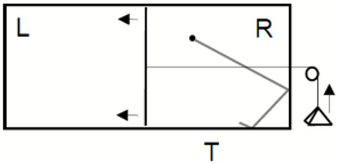
A naive calculation gives how much work it can extract

$$W={\int }_{V_i}^{2V_i}pdV={\int }_V^{2V}\frac{kT}{V}dV=kTln2$$

(12)

where we used the ideal gas equation $pV=NkT$ with $N=1$ and $V_i$ is the initial volume. Alternatively, but still somewhat naively, one may use the free energy of the state $F=U-TS$, where S is now $k_{B}ln2$ times the entropy to base 2 because of definitions of units. $\delta F=F_f-F_i$ is supposedly the optimal work that can be extracted isothermally at temperature T. By the equipartition principle the energy of the particle here, which is entirely kinetic, only depends on T ($kT/2=\langle 1/m{v}_x^2\rangle$), which is constant, so that $\delta F=T\delta S=kTln2$. This latter formula strongly suggests that more generally losing one bit, the L vs R information in this case, can give $kTln2$ of work.

The inverse process would be to invest work to reduce entropy. In this case the gas would be compressed. Resetting the L vs R bit isothermally would now cost at least $kTln2$ work; this is an instance of the famous Landauer principle [24] in action: it costs at least $kTln2$ of work to reset a bit (isothermally, on degenerate energy levels).

These were quick naive calculations, let us return later to this in more detail, but for now let us assume that one may say that there is a constant work gain $c_T$ possible if one hooks up the weight from the correct side. Let us in particular, and this assumption will only actually be physically valid under an additional assumption I will discuss later, assume that one can gain $c_T$ of work with probability 1 when connecting the divider correctly.

Now here is an example of a simple game. Assume that the agent has done its measurements, and assigned a state $\left[p\right(L),p(R\left)\right]$ to the particle’s (coarse-grained) position. There is some fixed final state, let us say $[1/2,1/2]$ which actually corresponds to the thermal state on the full box. The agent can connect the weight from whichever side it chooses and if it does it correctly it gains $c_T$ of work. So there are actually only two strategies to choose between: connect the weight from the right or from the left. The optimal is to connect it from the side with the higher probability. We see for example that, for $\epsilon >1-max\left(p\right(L),p(R\left)\right)$, $W^{\epsilon }=c_T=kTln2$. We see that an agent who knows the particle position can extract work at a lower risk of failure than someone who does not. Already in this simple example we must accept that the extractable work is subjective.

One may certainly worry about whether this game, where one gets $c_T$ with probability 1 if one guesses L vs R correctly, really corresponds to the physical setting of a single-atom gas in the Szilard engine. For example, as shown in [25], a numerical model of figure 4 using classical mechanics and the particle velocity getting picked from the Maxwell-Boltzmann distribution whenever it hits a wall, gives a very wide distribution in divider positions at the end, with $kTln2$ not being the average whether over time for a single box, or over many realizations of the same box. What happens is that when the particle is bouncing around away from the divider, the gravity pull on the weight accelerates the divider in one direction, until it gets knocked back the other way when the particle hits it. The divider position thus undertakes quite a violent and non-trivial random walk, and the process is certainly not quasi-static. There are two ways to get around this problem of the weight-divider system getting randomized: (i) One may consider [26] a set of n Szilard boxes sharing the same divider; this way the divider gets hit more of the time and its movements become approximately quasi-static for a sufficiently large number of particles, (ii) One may take the divider to have a speed independent of the interaction with the particle. This is the paradigm used for example in the context of Jarzynski’s equality, a different approach in non-equilibrium thermodynamics, and it is also a paradigm that we will adopt for a more sophisticated type of work extract game below. We will discuss in that section how work is defined in this case.

3.3. Multiple Szilard Engines

Bennett extended Szilard’s engine to a multi-cylinder version in the sense of having n such boxes [27]. Now one can do more interesting things than just flipping individual boxes. One can also imagine interacting them to perform for example a controlled-not gate (CNOT) which takes $\left[P\right(LL),P(LR),P(RL),P(RR\left)\right]\mapsto \left[P\right(LL),P(LR),P(RR),P(RL\left)\right].$ (It is called controlled not because it flips the second bit, called a NOT gate, if the first bit is a particular value, the NOT is controlled by the first bit). To visualize an idealized way of doing this one may imagine the particles in the two boxes are charged and repel each other when close. Then one takes the first box, rotates it 90 degrees and brings it close to the second one along the line that divides L and R for the second box, in such a way that only the right side of the first box is close to the second one. The second box can pivot on a nail through its centre, and the interaction with the first box can be timed such that the second box undergoes a flip $L⟷R$ if it feels the repulsion, which would be if the particle of the first box is in R. Importantly this needs not cost any energy as the energy of the final and initial states are identical in this case. It is moreover possible to implement reversibly in principle, as the laws of classical and quantum mechanics allow for reversible interactions. Consider an important example due to Bennett now: $[1/2,0,0,1/2]\mapsto [1/2,0,1/2,0]$. This allows us to take a case where we do not know whether either box is L or R to a case where we know that the second box is L. We can now extract, under the assumptions discussed above, $c_T=kTln2$ of work from the second box.

This suggests the following extension of the above game for a single box: allow the agent to (i) perform any permutation of bit strings, (ii) to connect any subset of boxes to the divider-weight system. This is the game which is at the centre of [1].

The strategy in the simple example above with two boxes uses both of these elementary steps. It can be called an information/randomness compression strategy because it concentrates the randomness onto one bit only. This kind of strategy can be used more generally on n boxes/bits to distill out a set of well-known bits from each of which $kTln2$ of work can be extracted. We can now see a connection to $S_{max}$: The minimal number of bits onto which the randomness can be pushed is given by $S_{max}$, so for such a strategy of optimal compression, $OpComp$, one can at most extract $(n-S_{max})kTln2$ of work with certainty: $W_{\text{OpComp}}^0=(n-S_{max})kTln2$.

3.4. Two-level Quantum System

This next game and variations on it was used in [2,3,6]. It is inspired by [28]. An a priori qualitatively different game is used in [4] although the expression for optimal work from there coincides with that derived in [3]. In this game there is a two-level quantum system, with each level being an energy eigenstate. The density matrix is taken to be diagonal in the energy eigenbasis, but the system will not be assumed to be in a thermal state at all times. This is consistent with taking the decoherence time to be much faster than the thermalization time.

Consider resetting a bit as in Landauer’s principle as depicted in Figure 5.

Figure 5. Landauer-style erasure/resetting of the state of a two-level quantum system with the Hamiltonian H=0 both initially and finally. An optimal protocol is to raise the second level isothermally and quasi-statically towards infinity, at a cost of $kTln2$, followed by a decoupling from the heat bath and a lowering of the second level back to 0 at zero work cost or gain.

Figure 5. Landauer-style erasure/resetting of the state of a two-level quantum system with the Hamiltonian H=0 both initially and finally. An optimal protocol is to raise the second level isothermally and quasi-statically towards infinity, at a cost of $kTln2$, followed by a decoupling from the heat bath and a lowering of the second level back to 0 at zero work cost or gain.

Now a quick free energy calculation also here suggests a cost of $kTln2$

$$W=\Delta U=0-T\Delta S=0-Tkln2=-Tkln2$$

(13)

Before proceeding, let us consider more carefully how to define work here. In the non-statistical setting, if a particle is in an energy level that is shifted by $\delta E$ it costs $\delta E$ work, energy taken from the work reservoir system. If a level is not occupied when it is shifted, no energy is needed to shift it. Now for an agent who does not know which state is occupied we have instead a probability distribution over levels and an associated probability distribution over the work cost of shifting an individual level.

The agent is also allowed to interact the system with a heat bath. This is modeled as only having the effect of changing the occupation probabilities, but not the energy eigenvalues. More specifically one assumes that the occupation probabilities evolve under a stochastic matrix which leaves the Gibb’s state ($\rho =e^{-\beta H}/Z$) invariant. Any energy change due to such a thermalization is not counted as work by definition.

These definitions of work and thermalizations fit nicely with the standard first law: The average work for the given shifts is $\langle \delta w\rangle ={\sum }_i{p}_i\delta E_i$. Note also that $\delta w$ has a neat ‘sister term’: we may write the change in internal energy as $\langle dU\rangle =d\left({\sum }_i{p}_{i}d{E}_i\right)={\sum }_i{p}_{i}d{E}_i+{\sum }_j\left(d{p}_j\right)E_j:=\langle dW\rangle +\langle dQ\rangle$. This extra sister term is then associated with interactions with a heat bath.

Now let us formulate the Landauer erasure case more clearly in this setting. The final and initial conditions are (i) the Hamiltonian is trivial, $H_i=H_f=0$ or in other words $E_1^i=E_2^i=E_1^f=E_2^f=0$, and (ii) The state goes from maximally mixed ${\rho }_i=1/2|e_1\rangle \langle e_1|+1/2|e_2\rangle \langle e_2|$, to pure ${\rho }_f=|e_1\rangle \langle e_1|$. The state is assumed to be diagonal in the energy eigenbasis at all times.

Strategy: (a) raise the second level an infinitesimal amount $d{E}_2$, then rethermalize the state. Repeat this to the limit as $E_2\to \infty$. (b) Then decouple from the heat bath and lower level 2 back to 0. The work cost of (a) is non-zero because it will frequently be the case that level 2 is occupied as it is raised. Step (b) is free as level 2 is unoccupied. The following argument gives the work cost of (a): if a level is occupied when raised by $\delta E_2$, it costs $dW=\delta E_2$ energy. If it is not occupied it is free to shift it. Thus

$$\langle d{W}_{Str}\rangle =p\left(E_1\right)0+p\left(E_2\right)d{E}_2=p\left(E_2\right)d{E}_2=\frac{exp(-\beta E_2)}{Z}d{E}_2$$

(14)

Thus

$${\langle W\rangle }_{Str.}={\int }_0^{\infty }\frac{exp(-\beta E_2)}{Z}d{E}_2=kTln2$$

(15)

(as can be seen from a few lines).

Importantly, the distribution of the work put in is a delta-function here, because every small energy raise can be broken up into infinitely many raises with each having the occupation probabilities picked independently. Then $\langle d{W}_{Str}\rangle$ and thus ${\langle W\rangle }_{Str.}$ is achieved with probability 1, as shown in [3] or alternatively using the McDiarmid inequality [29]. This means that in the notation used here, $W_{Str}^{\epsilon }=kTln2\forall \epsilon \in (0,1]$.

One should also note that, inversely, we could have extracted $kTln2$ by firstly raising the empty second level for free to infinity and then lowering it whilst thermalising (again the integration limits are simply switched). This would be the Szilard engine direction.

3.5. More General Game on Many Energy Levels

These examples suggest a more general game: we have some initial and final energies and some initial and final occupation probabilities of a set of energy levels. We can couple to the heat bath (this moves the occupation probabilities towards those of a thermal state), and we can move the energy levels up or down individually. $\delta E$ of energy is taken from the reservoir if a level is occupied when changed by $\delta E$.

Note that we have implicitly taken the paradigm (ii) mentioned in the section on the Szilard engine, by assuming that the energy level movements can be defined before the realization as part of the strategy. In particular they do not change as a function of the system’s state.

3.6. Expressions for Optimal Work

We now give an overview of the expressions that have been derived for optimal work in different games and discuss how they are related.

In [1] the n-cylinder Szilard engine game was considered and the following expression derived:

$$W^{\epsilon }=\left(n-S_{max}^{\epsilon }\right)kTln2$$

(16)

A key result obtained independently of each other in the more recent papers [3,4] is that given an initial state ρ taken to be diagonal in the energy eigenbasis, and a final thermal state ${\rho }_T$ over the same energy levels, the work that can be extracted given access to a heat bath of temperature T, and with up to ε failure probability is:

$$W^{\epsilon }=kTln\left(2\right)D_0^{\epsilon }(\rho ||{\rho }_T)$$

(17)

This reduces to $W=kTln\left(2\right)D(\rho ||{\rho }_T)$ for the standard relative entropy in the von Neumann regime. That latter expression is well-established, see e.g., [30]. Equation (17) reduces to Equation (16) in the case of degenerate energy levels, as shown in [3]. In [4] an expression is also given for the inverse process of taking a thermal state to any diagonal state with the same energy spectrum. In [5] the initial and final energy levels are arbitrary and the initial and final occupation probabilities are arbitrary. There it is proven that the optimal work is

$$W^{\epsilon }(\rho \to \sigma )=kTln\left(M\left(\frac{G^T\left(\rho \right)}{1-\epsilon }||G^T\left(\sigma \right)\right)\right)$$

(18)

where $G^T\left(\rho \right)$ is an operation termed Gibbs-rescaling [4,5,31,32,33]. This modifies the occupation probabilities in such a way that the bias on the energy levels imposed by the heat bath at temperature T are cancelled, so that e.g., a thermal state becomes a uniform distribution. $M(.||.)$, termed the relative mixedness, is a measure of how much one distribution majorises another one. A distribution $\overrightarrow{p}$ majorising another one $\overrightarrow{q}$ is written as $\overrightarrow{p}\succ \overrightarrow{q}$, and this is the case if and only if a doubly stochastic matrix $\mathcal{M}$ ‘connects’ them in the sense that $\overrightarrow{q}=\mathcal{M}\overrightarrow{p}$.

In the appropriate limits Equations (17) and (16) are recovered from Equation (18). This is somewhat surprising as in particular [4] has an a priori quite different model and moreover a subtly different definition of $W^{\epsilon }$. The agreement between the different results gives confidence that results are not too dependent on the specific assumptions of the derivations.

3.7. Quantum Memory

If one views the memory of the agent from the outside, the fact that the agent has information can be modeled as the joint state of the agent’s memory and the working medium system not being a product state: ${\rho }_{M,Sys}\ne {\rho }_M\otimes {\rho }_{Sys}$. This also begs the question of what can happen when the joint state is entangled. Such a scenario is called a quantum memory scenario. In [2,6] this is considered in the context of single-shot statistical mechanics.

In [2,6] the initial and final energy levels are all taken to have $E=0$. Consider firstly [2]. There is some initial ${\rho }_{M,Sys}$ and it is a Landauer-erasure type scenario in that the final state of the system is is set to $|0\rangle$. The memory system state has to be preserved however, so that the final state is chosen to be $|0\rangle \langle 0|\otimes {\rho }_M$ . This restriction makes it fair to say that any aid from the memory is only from its correlations with the system, i.e., the knowledge encoded in the memory. The agent can extract work via the many-level scheme above, and may extract it from the joint $MSys$ system (not just Sys). The paper [2] provides a strategy that performs this operation at a guaranteed work input of roughly $S_{max}(Sys|M)kTln2$, and [6] shows amongst other things that this is optimal. When the conditional entropy is negative, implying entanglement between Sys and M, it means work is extracted from this procedure.

Firstly consider a simple example to illustrate the protocol: Let the initial state be $\frac{1}{\sqrt{2}}(|00{\rangle }_{Sys,M}+|11{\rangle }_{Sys,M})$, such that $S(Sys|M)=-1$.

(1)

Extract $W_{\text{out}}=2kTln2$ work from both Sys and M.

(2)

Reset Sys to $|0\rangle$ by using $W=kTln2$ work.

Net result: Sys is reset and the reduced state on M is unchanged. The net work is given by

$$W=Win-Wout=-kTln2=S(A|Q)kTln2$$

(19)

It turns out this can be generalised to arbitrary states, in that the protocol gives essentially this work cost for all initial states.

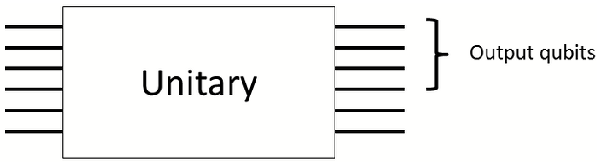
A fun (and at the moment hypothetical) application of this is cooling quantum computers, see Figure 6.

Figure 6. A unitary implementing Shor’s algorithm is implemented in circuit model computation. Not all qubits are measured in the end to get the output. We may extract work from correlations between the output qubits and the rest. After the proposed protocol the reduced state on the output qubits is invariant so the computation output is not affected. The energy extracted comes from the computer and its surroundings, so the computer is cooled.

Figure 6. A unitary implementing Shor’s algorithm is implemented in circuit model computation. Not all qubits are measured in the end to get the output. We may extract work from correlations between the output qubits and the rest. After the proposed protocol the reduced state on the output qubits is invariant so the computation output is not affected. The energy extracted comes from the computer and its surroundings, so the computer is cooled.

A take-away message from these games is that quantities from single-shot information theory emerge naturally if one asks how much work one is guaranteed to be able to extract in a given run of an experiment via an optimal extraction. The smoothing parameter ε also emerges naturally as the probability of failing to extract the amount of work in question.

3.8. Conceptual Questions

In the context of these games it is quite clear why subjective entropy can appear in the same equation as work. $W^{\epsilon }$ (or whichever such quantity one chooses) can certainly be different for different observers since different observers assign different states to the working medium in general, reflecting the fact that they can know different things about the working medium state. $W^{\epsilon }$ concerns the work extractable with a given certainty by a given observer.

4. Conclusions and Outlook

One can define work extraction games where it becomes a well-defined quantitative question as to how much work one can optimally extract as a function of one’s information about the working medium system. One does not need to assume that the states are thermal, they could also be states assigned by a Maxwell’s daemon who has extra knowledge. It is natural to employ single-shot information theory to calculate these expressions.

One should consider more general games: states that are not diagonal in the energy eigenbasis for non-degenerate Hamiltonians, quantum memory scenarios for non-degenerate energy levels, as well as other additional limitations such as limits on the time taken to implement the protocol or the level of experimental control of the agent.

One should also consider real experiments and how these strategies could be implemented in practice. This is likely to generate further theoretical questions in a constructive feedback process between experiment and theory.

Finally, I emphasize again that there will be several results and interesting arguments in the literature that are not in this note so I urge the readers to look into the references for further details.

Note added: after completing this note a further paper that contributes to this approach appeared on the arXiv [34].

References

- Dahlsten, O.C.O.; Renner, R.; Rieper, E.; Vedral, V. Inadequacy of von Neumann entropy for characterizing extractable work. New J. Phys. 2011, 13, 053015. [Google Scholar] [CrossRef]
- Rio, L.; Aberg, J.; Renner, R.; Dahlsten, O.; Vedral, V. The thermodynamic meaning of negative entropy. Nature 2011, 474, 61–63. [Google Scholar] [CrossRef] [PubMed]
- Aberg, J. Truly work-like work extraction. Nat. Commun. 2013, 4. [Google Scholar] [CrossRef] [PubMed]
- Horodecki, M.; Oppenheim, J. Fundamental limitations for quantum and nano thermodynamics. Nat. Commun. 2013, 4. [Google Scholar] [CrossRef] [PubMed]
- Egloff, D.; Dahlsten, O.C.O.; Renner, R.; Vlatko, V. Laws of thermodynamics beyond the von neumann regime. 2012; arXiv:1207.0434. [Google Scholar]
- Faist, P.; Dupuis, F.; Oppenheim, J.; Renner, R. A quantitative Landauer’s principle. 2012; arXiv:1211.1037. [Google Scholar]
- Maroney, O. Information processing and thermodynamic entropy. Available online: http://plato.stanford.edu/entries/information-entropy/ (accessed on 17 August 2013).
- Baldo, M. Introduction to Nanoelectronics; MIT OpenCourseWare, License; Creative Commons BY-NC-SA; Massachusetts Institute of Technology: Cambridge, MA, USA, 2012; Available online: http://ocw.mit.edu (accessed on 30 July 2013).
- Frank, M.P. Approaching the Physical Limits of Computing. In Proceedings of IEEE 35th International Symposium on Multiple-Valued Logic, Piscataway, NJ, USA, 19–21 May 2005; pp. 168–185.
- Jarzynski, C. Nonequilibrium equality for free energy differences. Phys. Rev. Lett. 1997, 78, 2690–2693. [Google Scholar] [CrossRef]
- Lloyd, S. Quantum-mechanical Maxwell’s demon. Phys. Rev. A 1997, 56, 3374–3382. [Google Scholar] [CrossRef]
- Gemmer, J.; Mahler, G. Quantum Thermodynamics: Emergence of Thermodynamic Behavior Within Composite Quantum Systems; Lecture Notes in Physics; Springer: Berlin, Germany, 2004. [Google Scholar]
- Allahverdyan, A.E.; Balian, R.; Nieuwenhuizen, T.M. Maximal work extraction from finite quantum systems. Europhys. Lett. 2004, 67, 565–571. [Google Scholar] [CrossRef]
- Linden, N.; Popescu, S.; Skrzypczyk, P. How small can thermal machines be? The smallest possible refrigerator. Phys. Rev. Lett. 2010, 105, 130401. [Google Scholar] [CrossRef] [PubMed]
- Brandão, F.G.S.L.; Horodecki, M.; Oppenheim, J.; Renes, J.M.; Spekkens, R.W. The resource theory of quantum states out of thermal equilibrium. 2011; arXiv:1111.3882. [Google Scholar]
- Jennings, D.; Rudolph, T.; Hirono, Y.; Nakayama, S.; Murao, M. Exchange fluctuation theorem for correlated quantum systems. 2012; arXiv:1204.3571. [Google Scholar]
- Toyabe, S.; Sagawa, T.; Ueda, M.; Muneyuki, E.; Sano, M. Experimental demonstration of information-to-energy conversion and validation of the generalized Jarzynski equality. Nat. Phys. 2010, 12, 988–992. [Google Scholar] [CrossRef]
- Renner, R. Security of quantum key distribution. 2005; arXiv:quant-ph/0512258. [Google Scholar]
- Cover, T.M.; Thomas, J.A. Elements of Information Theory; Wiley Series in Telecommunications and Signal Processing; Wiley: New York, NY, USA, 1991. [Google Scholar]
- Tomamichel, M.; Colbeck, R.; Renner, R. A fully quantum asymptotic equipartition property. IEEE Trans. Inf. Theory 2009, 55, 5840–5847. [Google Scholar] [CrossRef]
- Datta, N. Min- and max-relative entropies and a new entanglement monotone. IEEE Trans. Inf. Theory 2009, 55, 2816–2826. [Google Scholar] [CrossRef]
- König, R.; Renner, R.; Schaffner, C. The operational meaning of min- and max-entropy. IEEE Trans. Inf. Theory 2009, 55, 4337–4347. [Google Scholar] [CrossRef]
- Szilárd, L. Über die Entropieverminderung in einem thermodynamischen System bei Eingriffen intelligenter Wesen. Zeitschrift für Physik 1929, 53, 840–856. (in German). [Google Scholar] [CrossRef]
- Landauer, R. Irreversibility and heat generation in the computing process. IBM J. Res. Dev. 1961, 5, 183–191. [Google Scholar] [CrossRef]
- Browne, C. EPSRC summer project, Oxford 2012, Discussions with J. Aberg. 2012. [Google Scholar]
- Zurek, W.H. Maxwell’s demon, Szilard’s engine and quantum measurements. 2003; arXiv:quant-ph/0301076. [Google Scholar]
- Bennett, C.H. Notes on Landauer’s principle, reversible computation, and Maxwell’s demon. Stud. Hist. Philos. Sci. B 2003, 34, 501–510. [Google Scholar] [CrossRef]
- Alicki, R.; Horodecki, M.; Horodecki, P.; Horodecki, R. Thermodynamics of quantum information systems—Hamiltonian description. Open Syst. Inf. Dyn. 2004, 11, 205–217. [Google Scholar] [CrossRef]
- McDiarmid, C. On the Method of Bounded Differences; London Mathematical Society Lecture Note Series 141; Oxford University: Oxford, UK, 1989; pp. 148–188. [Google Scholar]
- Donald, M. Free energy and the relative entropy. J. Stat. Phys. 1987, 49, 81–87. [Google Scholar] [CrossRef]
- Ruch, E.; Mead, A. The principle of increasing mixing character and some of its consequences. Theor. Chim. Acta 1976, 41, 95–117. [Google Scholar] [CrossRef]
- Ruch, E. The diagram lattice as a structural principle. Theor. Chim. Acta 1975, 38, 167–183. [Google Scholar] [CrossRef]
- Mead, C.A. Mixing character and its application to irreversible processes in macroscopic systems. J. Chem. Phys. 1977, 66, 459–467. [Google Scholar] [CrossRef]
- Gour, G.; Müller, M.P.; Narasimhachar, V.; Spekkens, R.W.; Yunger Halpern, N. The resource theory of informational nonequilibrium in thermodynamics. 2013; arXiv:1309.6586. [Google Scholar]
© 2013 by the author; licensee MDPI, Basel, Switzerland. This article is an open access article distributed under the terms and conditions of the Creative Commons Attribution license (http://creativecommons.org/licenses/by/3.0/).
Share and Cite
MDPI and ACS Style
Dahlsten, O.C.O. Non-Equilibrium Statistical Mechanics Inspired by Modern Information Theory. Entropy 2013, 15, 5346-5361. https://doi.org/10.3390/e15125346
AMA Style
Dahlsten OCO. Non-Equilibrium Statistical Mechanics Inspired by Modern Information Theory. Entropy. 2013; 15(12):5346-5361. https://doi.org/10.3390/e15125346
Chicago/Turabian StyleDahlsten, Oscar C. O. 2013. "Non-Equilibrium Statistical Mechanics Inspired by Modern Information Theory" Entropy 15, no. 12: 5346-5361. https://doi.org/10.3390/e15125346