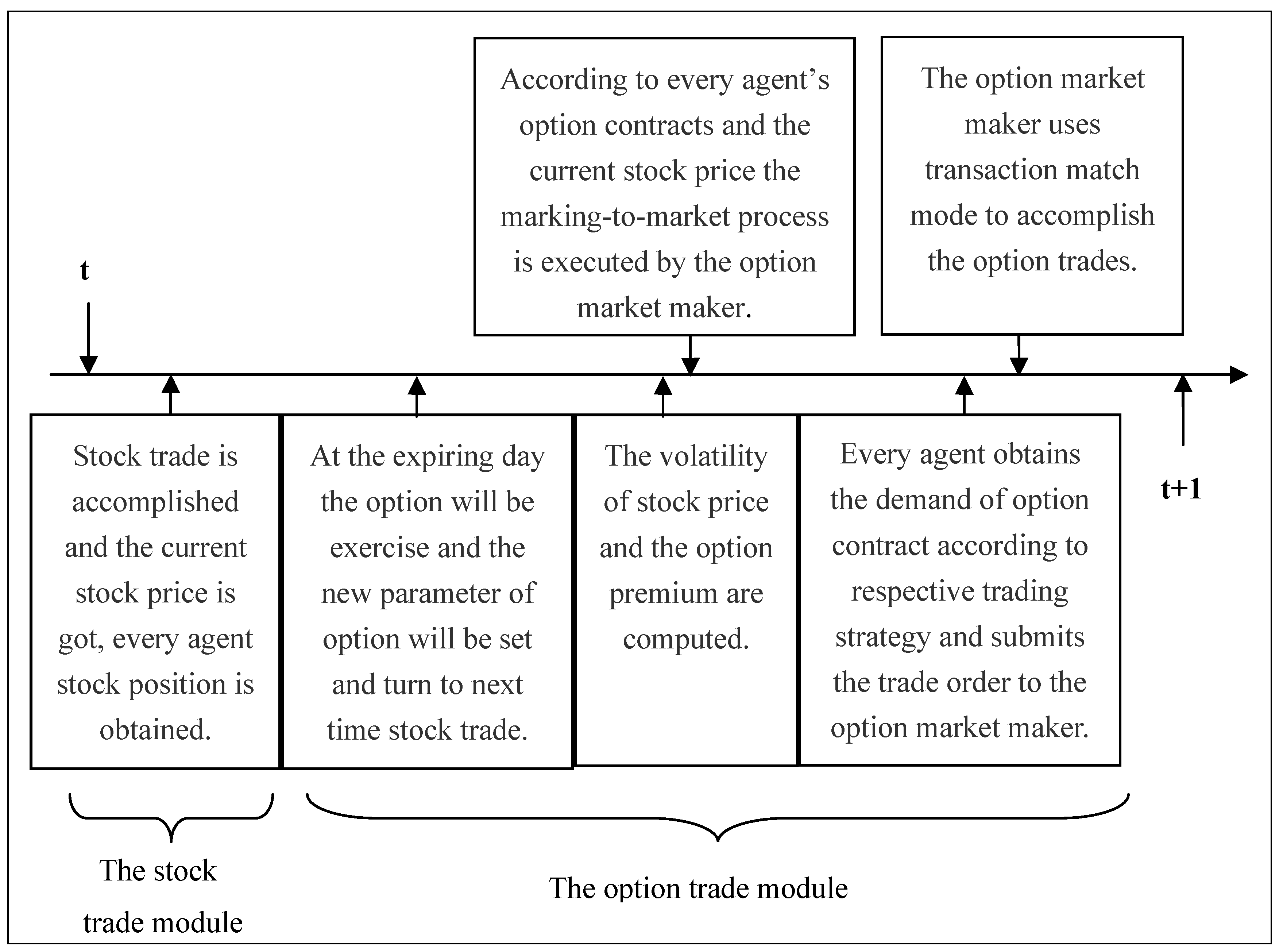
In this section we focus on the new model which includes two modules. First, the stock trade module will be introduced and its limitations will be pointed out. Second, the compound Poisson process will be employed to describe the dividend process. Finally, the option trade module will be presented.
Figure 4.
The time line of a market day (the X-axis represents time).
3.2. The Stability of the Model
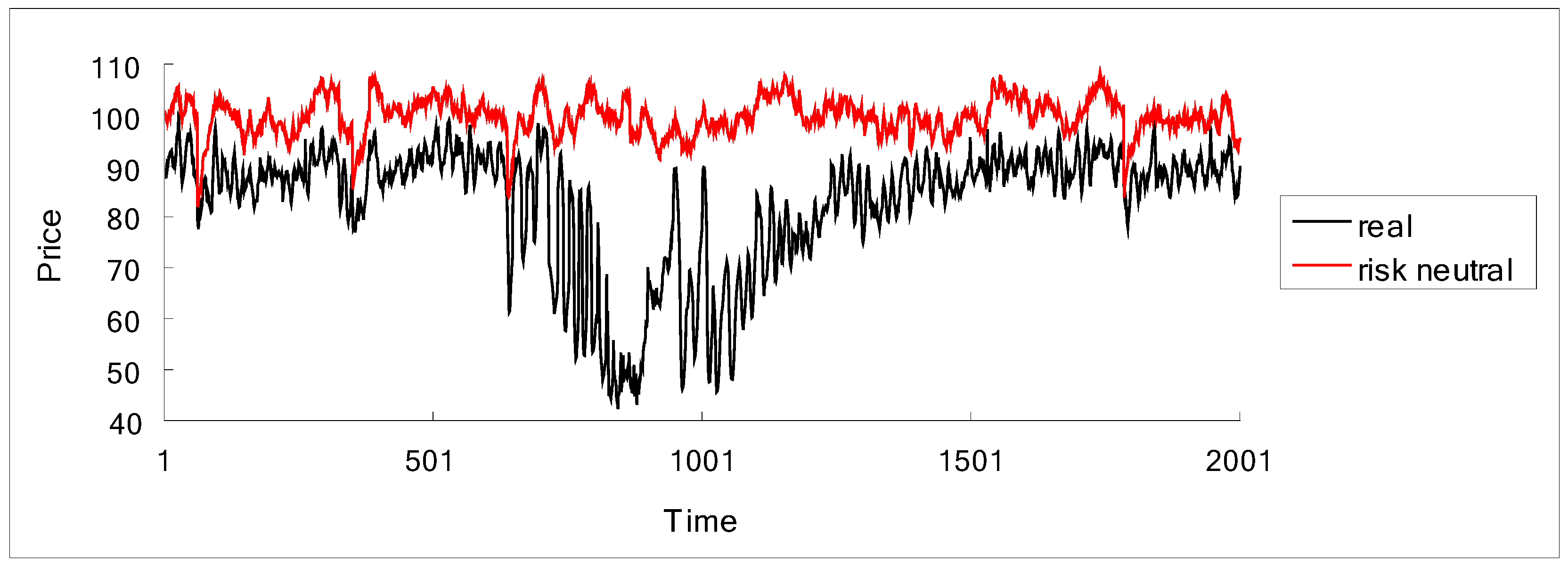
Before comparing in detail the differences between the stock market and the option market, we first analyze the stability of model with options. In the experiment after the running period of the stock trade module equals 5,000 the option trade module starts to run. The model is executed more than 200,000 periods without any interruption.
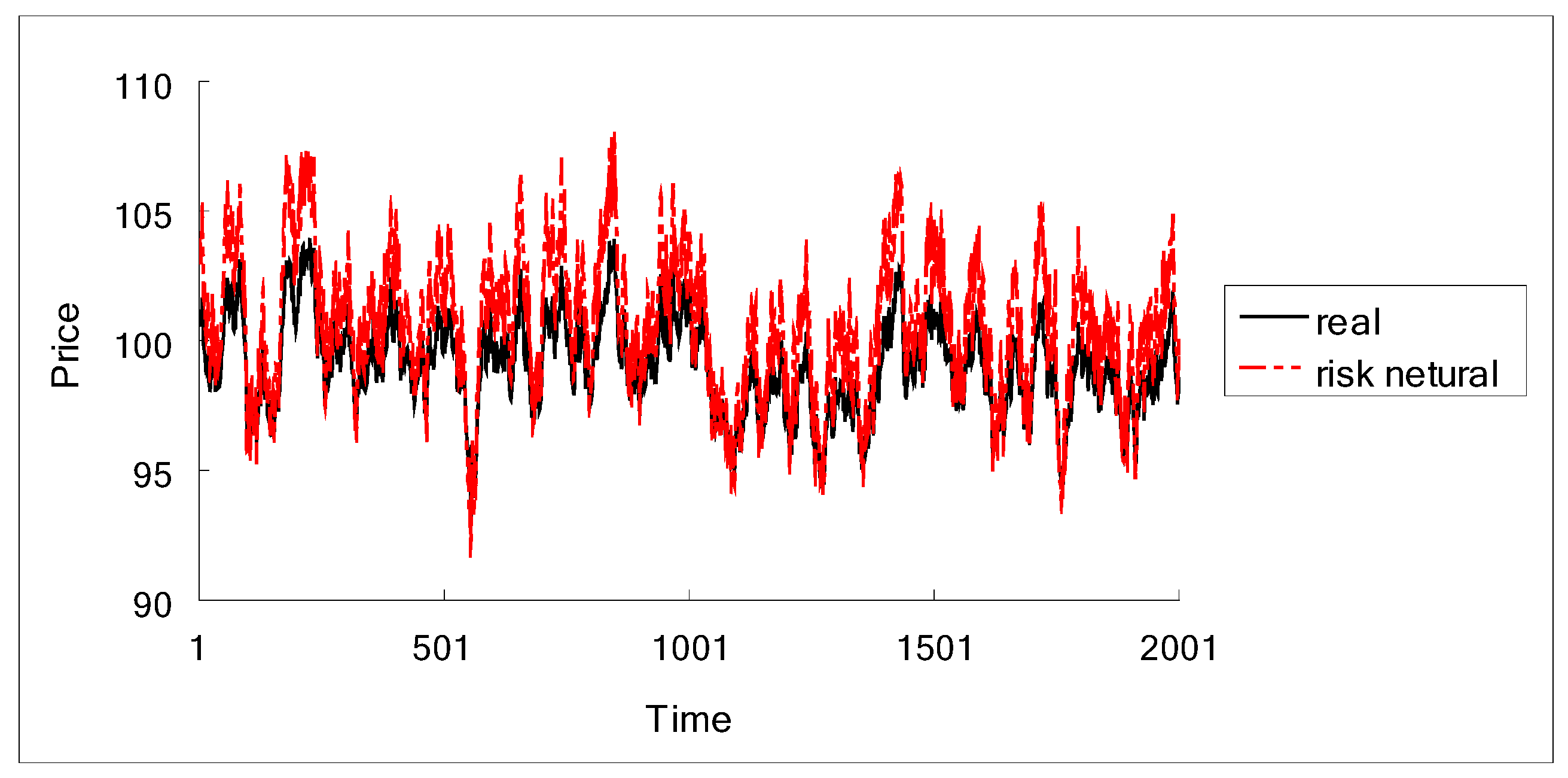
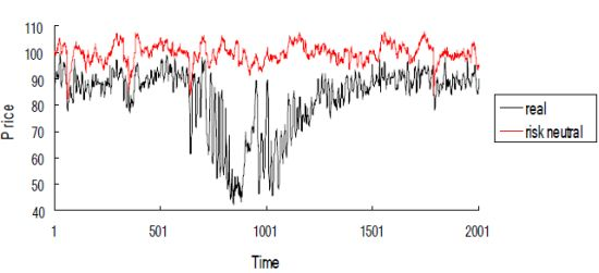
Figure 5 is price time series of stock from the 0th period to the 20,000th period. In
Figure 5 “real” price represents the price obtained through stock trade, “risk neutral” price represents the price obtained by equation (
).
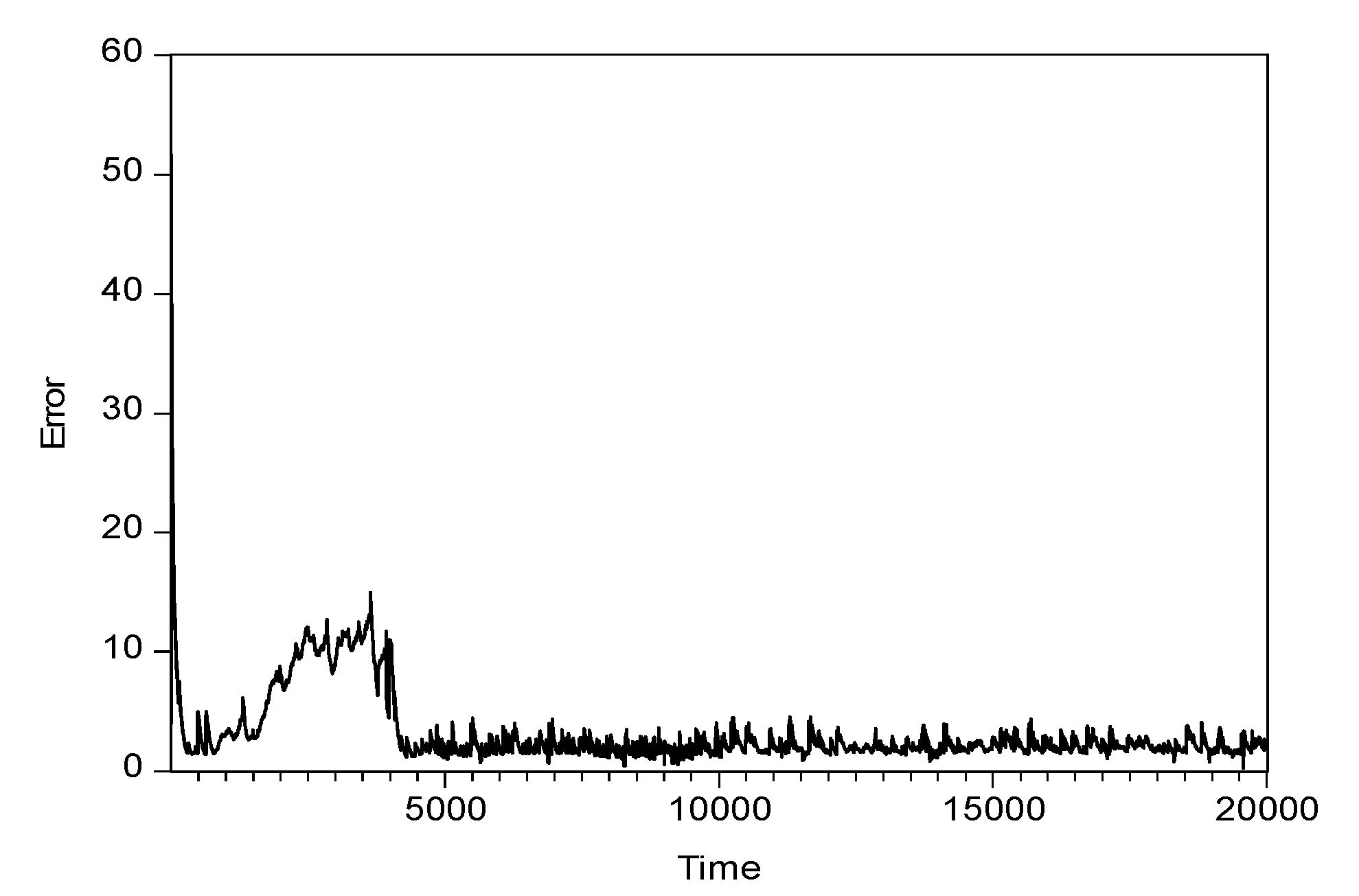
Figure 6 is the forecast error time series of stock price of the first agent from the 0th to the 20,000th period, the forecast errors of stock price of the other agents have the same change tendency.
Figure 5.
The price time series of stock.
Figure 5.
The price time series of stock.
Figure 6.
The forecast error time series of stock price of the first agent.
Figure 6.
The forecast error time series of stock price of the first agent.
From
Figure 5 and
Figure 6 we can see that the system remains stable from the 5,000th period. When the stock option starts to trade at the 10,000th one, the time series has not obviously changed and the system continues to remain stable. The forecast error becomes very small as the stock price tends to stabilize and after 50,000th period the forecast error of every agent is less than 2.0.
3.3. The Effect of Option Market on Stock Price and Volume
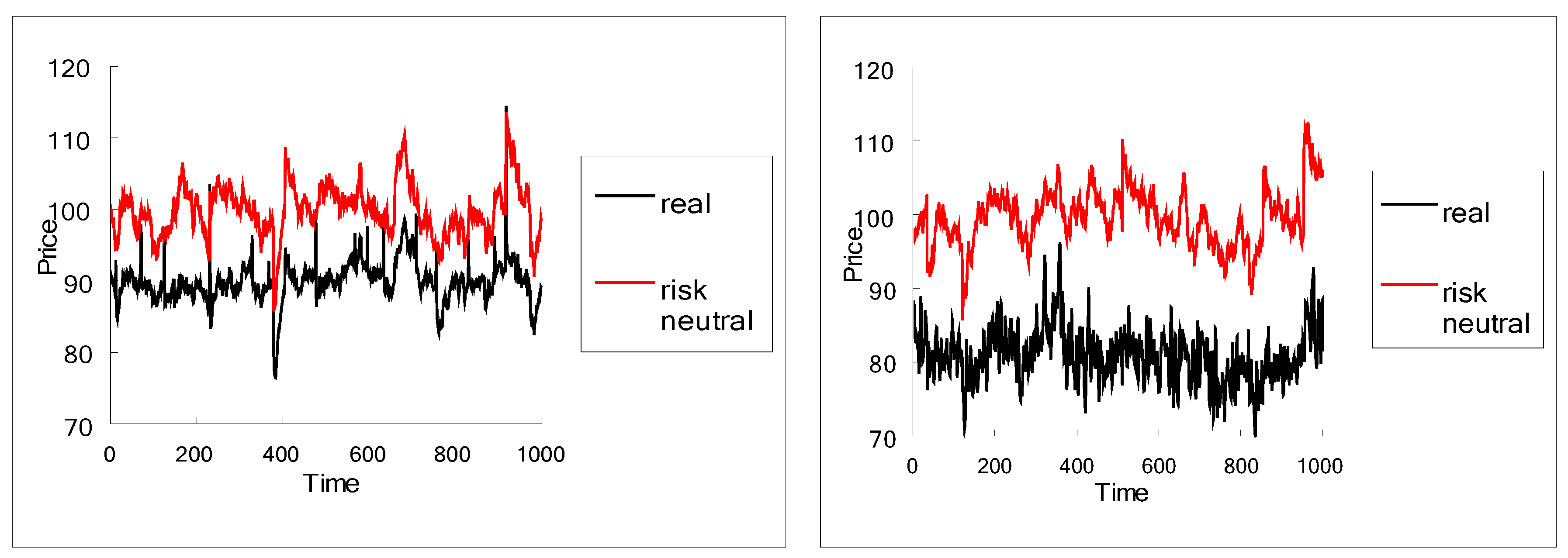
Next we will analyze the effect of the option market on the stock market. So as to compare directly, the 100,000th period is taken as a transition point. Before the 100,000th period, the option trade is not included and after 100,000th period the option trade starts to run.
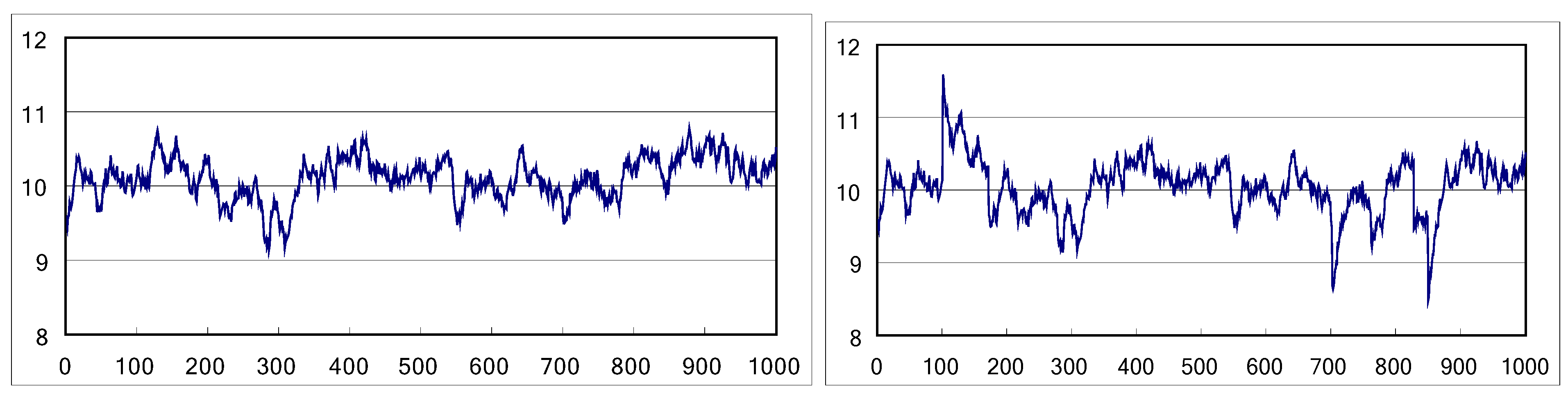
Figure 7 illustrates the stock price time series which are chosen from a long stable price sequence. From
Figure 7, we can find the obvious difference between the two cases. After the option is introduced, the price volatility becomes higher and the spread of the real price and the risk neutral price becomes larger. The result implicates that option information (price and volume) impacts on the real price of stock. That is to say, the option market affects the stock market by information diffusion through the network.
Figure 7.
The price time series of stock. (left: before the option is introduced; right: after the option is introduced).
Figure 7.
The price time series of stock. (left: before the option is introduced; right: after the option is introduced).
From the statistical data of
Table 6, we can find the obvious difference between the two states, especially in variances. From the stock price, we can find that the average of stock price decreases after the stock option starts to trade. However, variance decreases more, which fits the fact that the higher the income, the greater the risk. A stock’s yield is the dividend per share divided by its current price per share. Before the option is introduced in the model, the stock average yield equals the average dividend divided by stock price. The value equals to 11.13% (10.0/89.81). After the option is introduced, the stock average yield is 12.48% (10.0/80.12).
Table 6.
The statistics of dividend and stock price.
Table 6.
The statistics of dividend and stock price.
| Stock price without option | Stock price with option | Trade volume without option | Trade volume with option |
|---|
| Average | 89.81 | 80.12 | 14.81 | 11.96 |
| Variance | 10.40 | 20.31 | 230.12 | 115.98 |
When average trading volume decreases, the variance also decreases, unlike the change in price. The increase of risk in owning the stock and the relatively unstable stock price causes the agents to tend to hold cash. This decreases both the variance of the trade volume and the average of trade volume.
The preceding analysis illustrates that the introduction of stock options cannot stabilize market price, so the variance of price increases. Therefore, the risk in owning stock becomes large, which leads to a decrease in the price of the stock. However, it should be pointed out that our conclusion is drawn based only on our model. Before the option is introduced, the stock trade module has reached the REE, though the compound Poisson process is introduced.
3.4. The Effect of Option Market on Stock Return and Volatility
This section mainly studies the changes of the features of stock return series market when the option market is introduced. The features of stock return include volatility persistence and fat tails or excess kurtosis.
At frequencies of less than one month, the unconditional returns of financial series are not normally distributed in the real market. They usually display a distribution with too few in the mid-range, too many observations near the mean, and again, too many in the extreme left and right tails. This feature discovered by Mandelbrot [
23] has puzzled financial economists. Recently, return distribution has obtained more attention in risk management because the computation of value at risk of stock needs relative correct return distributions.
Stock returns are normally calculated by the following expression,
,
is the current stock price. But in our model the computation of stock return needs to be adjusted because a dividend is paid each period, which is not common in the real stock market. The stock dividend is also paid, but time intervals are far longer. In our model we use
to calculate the stock returns;
dt denotes the current stock dividend.
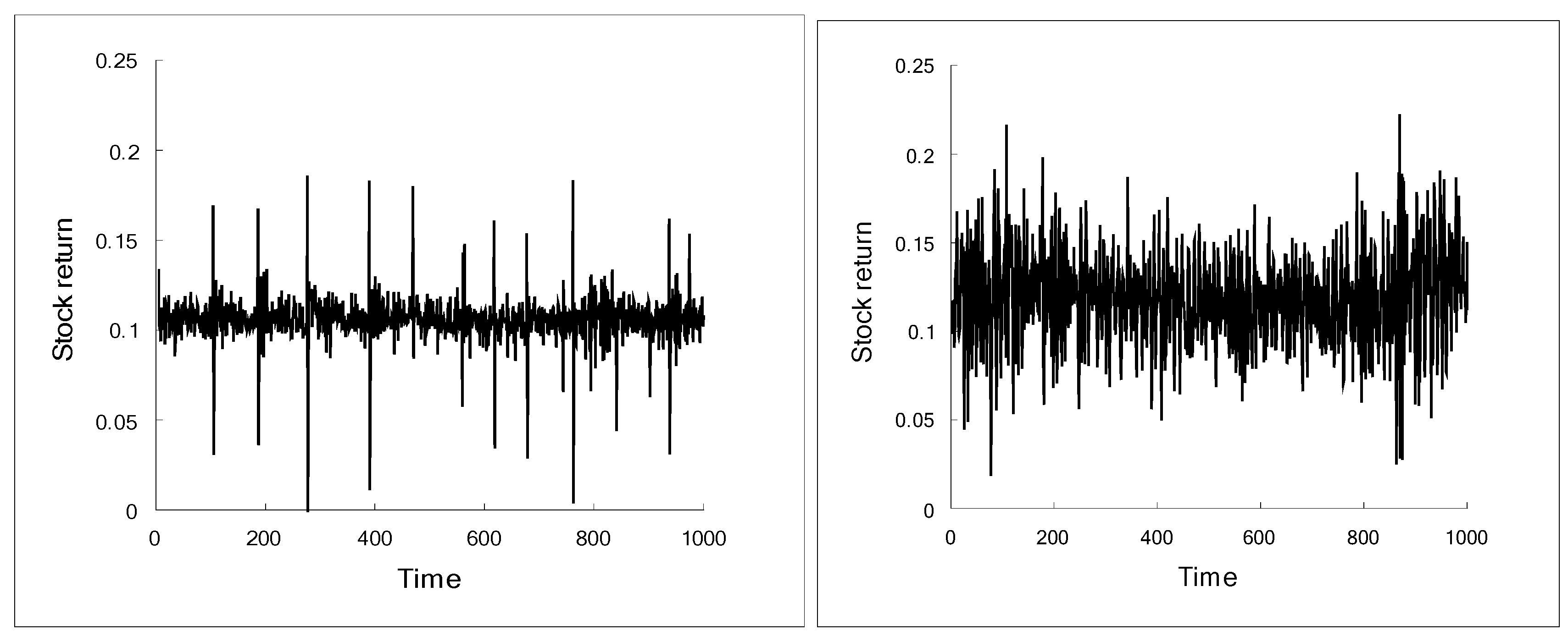
Figure 8 is stock price return time series which are chosen in a long stable price sequence. The sample size in
Table 7 is 50,000.
Figure 8.
The time series of stock logarithmic returns. (left: before the option is introduced; right: after the option is introduced).
Figure 8.
The time series of stock logarithmic returns. (left: before the option is introduced; right: after the option is introduced).
Table 7.
The statistics of dividend and stock logarithmic return.
Table 7.
The statistics of dividend and stock logarithmic return.
| Stock return without option | Stock return with option |
|---|
| Average | 0.105579 | 0.120366 |
| Variance | 0.000346 | 0.000937 |
| Kurtosis | 22.1443 | 14.49292 |
From
Figure 8 and
Table 7 we can find that the difference between the two stock returns obviously. Before the option is introduced, the stock returns change gently as a whole, because of the introduction of the compound Poisson process. There are some sudden changes in the stock return, which makes the kurtosis become very large. After the option is introduced, the average stock return and volatility increase, but the kurtosis also decreases. The shape of stock return is closer to the real stock return. Stock return distributions show obvious fat tails or excess kurtosis (kurtosis > 3) whether or not the stock option is introduced. The results show that the excess kurtosis and fat tail has nothing to do with the introduction of options. In addition, option trading really has an impact on the return of stock. Conversely, the fluctuation of stock price can continually affect the option market.
Next we will analyze the volatility of the stock which is an important parameter in the stock market. Volatility cannot be observed directly, but it has some important features such as the persistence of volatility that lacks a widely accepted explanation. In order to analyze the volatility, we use the conditional volatility models which seem to be appropriate.
The GARCH model was proposed initially by Bollerslev [
24]. The GARCH model largely consists of two parts, the mean equation and conditional variance covariance equations. The mean equation used in the paper is ARMA model. The conditional variance covariance equations used is the GARCH(1,1) model which has been proven to be an adequate representation for most financial time series by Lamoreux and Lastrpes [
25]:
where
follows
,
follows
,
.
We firstly build the ARMA model by using EVIEWS software measurement model parameter estimation and testing. The parameters of the ARMA model are as shown in
Table 8 and
Table 9.
Table 8.
The parameters of ARMA model before option is introduced.
Table 8.
The parameters of ARMA model before option is introduced.
| Variable | Coefficient | Std. Error | t-Statistic | Prob. |
|---|
| C | 0.105579 | 5.28E−05 | 2000.599 | 0.0000 |
| AR(1) | −0.138857 | 0.012371 | −11.22476 | 0.0000 |
| MA(1) | −0.232591 | 0.012149 | −19.14488 | 0.0000 |
Table 9.
The parameters of ARMA model after option is introduced.
Table 9.
The parameters of ARMA model after option is introduced.
| Variable | Coefficient | Std. Error | t-Statistic | Prob. |
|---|
| C | 0.119826 | 0.000857 | 139.7441 | 0.0000 |
| AR(1) | 1.718534 | 0.011286 | 152.2778 | 0.0000 |
| AR(2) | −0.51085 | 0.023445 | −21.7891 | 0.0000 |
| AR(3) | −0.61926 | 0.01682 | −36.8165 | 0.0000 |
| AR(4) | 0.409515 | 0.004987 | 82.11901 | 0.0000 |
| MA(1) | −1.53815 | 0.012256 | −125.502 | 0.0000 |
| MA(2) | 0.392182 | 0.023032 | 17.0278 | 0.0000 |
| MA(3) | 0.16174 | 0.011836 | 13.66452 | 0.0000 |
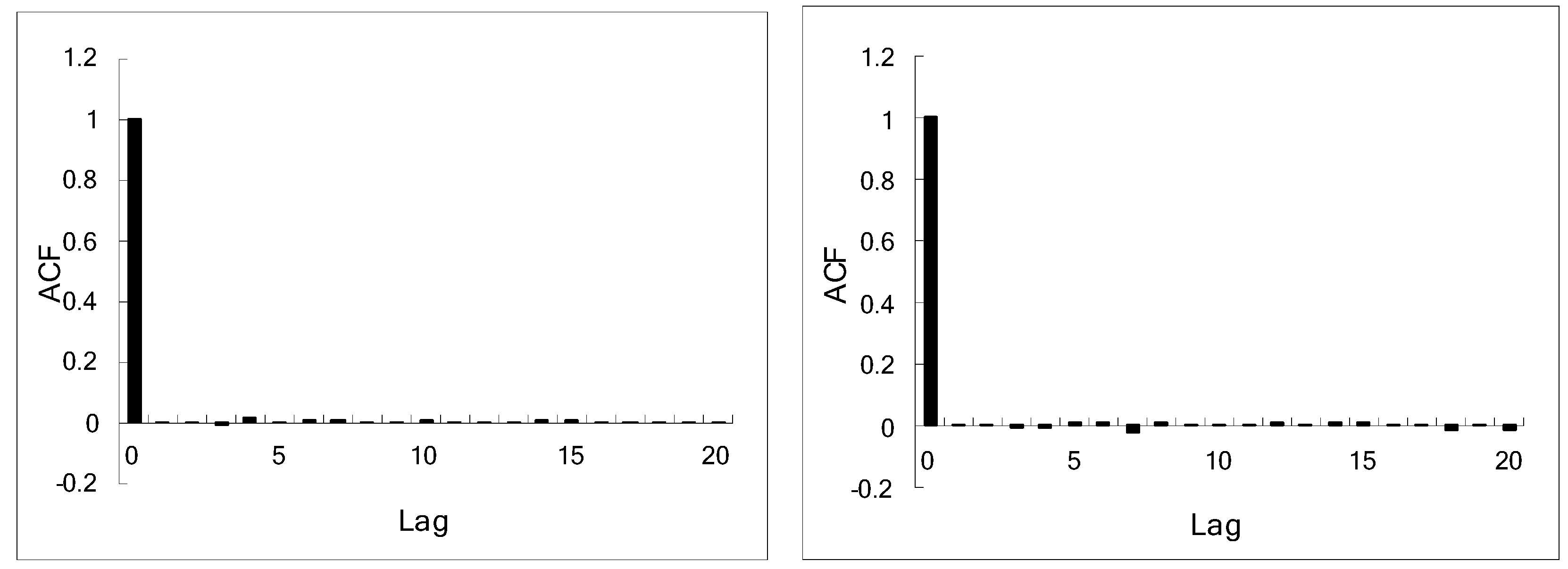
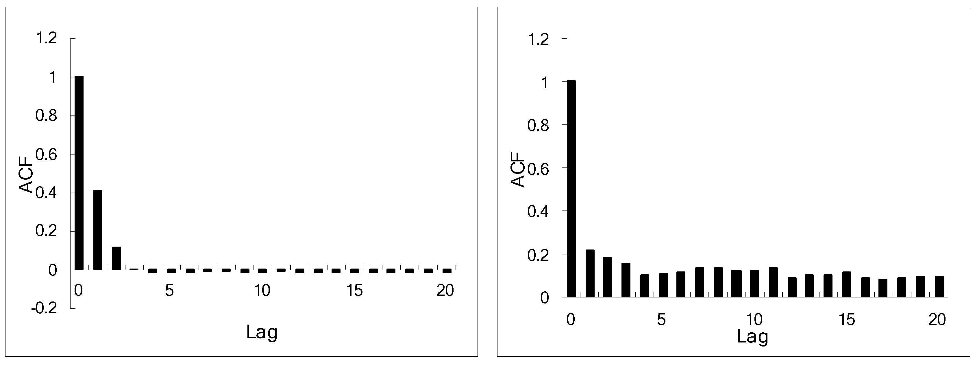
In
Figure 9 and
Figure 10, the stock return residual refers to the residual after the ARMA is built. From
Figure 9 we can see that the Serial correlation of the residual doesn’t exist after the ARMA is built. Conversely, in
Figure 10 the Serial correlation of residual squares does exist, which shows that the ARCH effect exits in the stock return series. To analyze this observation objectively, we carry out the statistical test of the ARCH effect. Like the results displayed in
Figure 9 and
Figure 10, the statistical test results show that there is an ARCH effect in the logarithmic return series and the results passed the significance test at the 1% level.
Figure 9.
The autocorrelation of the stock return residual series. (left: before the option is introduced; right: after the option is introduced).
Figure 9.
The autocorrelation of the stock return residual series. (left: before the option is introduced; right: after the option is introduced).
Figure 10.
The autocorrelation of the stock return residual squared series. (left: before the option is introduced; right: after the option is introduced).
Figure 10.
The autocorrelation of the stock return residual squared series. (left: before the option is introduced; right: after the option is introduced).
The specific parameters of the model are in
Table 10 and all parameters pass the 1% significance level test.
Table 10.
The parameters of GARCH (1,1) model.
Table 10.
The parameters of GARCH (1,1) model.
| Parameters | | | |
|---|
| Before | 0.000168 | 0.429756 | −0.00509 |
| After | 1.62E−05 | 0.058384 | 0.914057 |
From
Table 10, we can see that the stock’s volatility persistence is clearly demonstrated through the ARMA-GARCH(1,1) model, whether the option is introduced or not. Yet the results also show that after the stock option is introduced, the parameters of ARMA-GARCH(1,1) model have changed. Because the purpose of the introduction of GARCH model is to analyze return volatility, we mainly focus on conditional variance covariance equation. The sizes of the
α1 and
β1 coefficients represent the strength of volatility persistence. After the option is introduced the
α1 value decreases, but the
β1 increases more, so in general, return volatility persistence becomes more obvious following the introduction of the option. Furthermore, more information has been transmitted from option market to stock market which is the reason of increases of volatility in stock market.
3.6. The Effect of Various Proportions of Option Traders
In this subsection we focus on the effect of the proportions of option traders. Parameter
γ equals 0.02, the length of information is 6 and the agent number is 200. The other parameters are the same as those in
Table 4.
In real financial markets there are different kinds of option traders whose purposes are different and whose strategies are relative complicated. So as to more closely represent a real market, there are three types of option trader in this model. Their option trade strategies are different and relatively simplified.
In
Table 14 the expression “0.15-0.15-0.35-0.35” represents the proportion of four types of option traders which are non-option traders, random option traders, hedge option traders and speculate option traders, respectively. In
Table 14 the other expressions have similar meanings. In the experimental design, we pay much more attention to the speculative option trader and the hedge option trader than to the non-option trader and the random option trader, so many experiments will be done about the proportion changes of two types of agents changes. The sample size is 50,000.
Table 14.
The statistics of stock price under different proportion of option traders.
Table 14.
The statistics of stock price under different proportion of option traders.
| Proportion | Average | Variance | Proportion | Average | Variance |
|---|
| 0.25-0.25-0.25-0.25 | 87.197 | 63.410 | 0-0-0.6-0.4 | 91.510 | 13.661 |
| 0.15-0.15-0.35-0.35 | 88.038 | 48.726 | 0-0-0.5-0.5 | 89.389 | 16.170 |
| 0.05-0.05-0.45-0.45 | 89.737 | 16.555 | 0-0-0.4-0.6 | 89.394 | 14.506 |
| 0-0-0.9-0.1 | 98.431 | 12.975 | 0-0-0.3-0.7 | 89.125 | 14.016 |
| 0-0-0.8-0.2 | 97.487 | 12.718 | 0-0-0.2-0.8 | 89.371 | 14.180 |
| 0-0-0.7-0.3 | 96.462 | 13.062 | 0-0-0.1-0.9 | 89.359 | 16.088 |
Table 14 shows that the changing proportion of traders does influence the stock market. Decreasing the non-option traders and random option traders can stabilize the stock market. The system becomes stable when the non-option and random option traders are less than 5%, respectively. Under these conditions, the variance rapidly decreases and the average price increases. This shows that as more people participate in stock option trading, with the exception of random traders, the stock market becomes more stable. The random option trader is a negative factor to stabilization of the stock market. Increasing proportions of this type of trader can make stock market more volatile. We can draw a conclusion that random option trader is a significant factor of the system stable because it transmit noise between option market and stock market. The noise not only is diffused among agents in the option market, but also transmitted in the stock market.
From the proportion of the hedge and speculate option traders the result shows that the increase of hedge option traders can stabilize the stock market. Conversely, the increase of speculate option traders can make the stock market more volatile, which fits the fact existing in the real financial market, so the correctness of the constructed models is proved.


