Exploring the Characteristics of Innovation Adoption in Social Networks: Structure, Homophily, and Strategy

Abstract

Exploration of the characteristics of innovation adoption in the context of social network will add new insights beyond the traditional innovation models. In this paper, we establish a new agent-based model to simulate the behaviors of agents in terms of innovation adoption. Specifically, we examine the effects of the network structure, homophily and strategy, among which homophily is a new topic in this field of innovation adoption. The experiments illustrate six important findings involving five aspects and their influences on the innovation adoption. The five aspects are initial conditions, homophily, network topology, rules of updating and strategy, respectively. This paper also compares the different cases within one aspect or across several aspects listed above. Accordingly, some management advices and future work are provided in the last part of this paper.

1. Introduction

Diffusion of innovation refers to the spread of new ideas, technologies, and practices within a social system [1], and specifically, innovation adoption is one form of innovation diffusion. Since networks form the backbone of social and economic life [2], viewing innovation adoption in the context of social networks will add a new insight beyond the traditional innovation adoption models. Firstly, given that structure analysis is one main topics in social network research [3], there are likely fundamental adoption characteristics related to how the social network is structured. For example, a random network has a different link mechanism than a small world network; as a result, the two kinds of networks would have different interpersonal contact efficiencies and accordingly different rates of innovation adoption. Secondly, homophily, i.e., the tendency of people to associate with others similar to themselves is observed in many social networks [4]. The considerable homophily among the members of a social network with regards to their attitudes on the given innovation will have an effect on their behaviors, in other words, the features caused in networks by homophily have significant consequences for the process of innovation diffusion and adoption [5]. For example, early adopters of an innovation tend to have a limited set of interactions within a social network and they have different behaviors than late adopters, in contrast to the traditional assumption that everyone has an equal chance of interacting with everyone else in the network [6,7]. Thirdly, when making decisions about adopting an innovation, members in a social network can use different strategies, which may cause different adoption times (the time when the system reaches its equilibrium) and adoption rates (the proportion of agents who adopt the innovation). For example, a member can decide whether to adopt a given innovation only based on his or her current situation such as the present benefit from adoption, in contrast that based on the others’ reactions to his or her possible adoption may be. The above three factors are summarized as “structure”, “homophily”, and “strategy”, consistent with the title of this paper. Besides, these three factors are also seen as controllable variables in this model when their effects on the innovation adoption are studied.

The goal of this paper is to explore the characteristics of innovation adoption in social networks, especially to uncover how the fundamental features of the social network influence the innovation adoption process. It is noted that we assume that one kind of innovation product exists in the system and all agents are aware of the product from the very beginning. What is focused on in this paper is the agents’ decision, which has network externalities, to adopt the innovation since these agents may have different judgments on the innovation. Accordingly, when the innovation adoption is mentioned hereinafter, it means the agents’ adoption decision. Specifically, how does the structure of social network affect adoption of a given innovation? In terms of the regular network, the random network, the small-world network and the scale-free network, which one has the highest adoption rate? And which one has the shortest adoption time? Although these basic problems have been studied by many papers such as Stephen and Catherine [8], Soumya, et al. [9], Peng and Mu [10], Centola and Macy [11], and Centola [12], they cannot be omitted for their significance, especially when they are studied under the condition of a new model different with the traditional ones and when they are studied combined with other factors such as the homophily and the decision-making strategy presented in this paper. Also, homophily always has distinguished sources such as race, age, gender, religion, education and so on, and the homophily appearing in the social network of innovation adoption is no exception. The fact can provide us new insights about how the homophily affects the innovation adoption, especially when the homophily has different sources and is differently defined. Luckily, the paper by Currarini, et al. [13] provides a wonderful tool and method to analyze and solve the problem. Besides, decision-making strategy of agents in the social network is critical to influence the dynamics of innovation diffusion [14]. Given two different adoption strategies, the time to reach the steady state of the adoption in the social network and the terminal steady-state adoption rate will be compared in the following part of this paper. The last not the least, it is also studied in this paper that how the initial conditions affect the steady-state adoption rate. In fact, the problem is often neglected in the existing literature about innovation diffusion and innovation adoption such as Anand, et al. [15], Renana, et al. [16], Sebastiano, et al. [17], and so on. One possible explanation is the models appearing in some of the above literatures are neutral to the initial conditions and so there is no need to analyze them, but the model presented in this paper has another story so that it is necessary to study the effect of initial values on the final state of the dynamic system.

To solve the above problems, a new agent-based model including the influence of different types of social networks topologies, the effect of homophily defined differently, and the impact of different strategies is presented. The main classical innovation diffusion model is the Bass model [18], and various extensions of the Bass model have been developed over the years, for example, Turk and Trkman [19], Dragan [20], and Sandberg [21]. However, a fundamental weakness of the Bass model is its assumption of homogeneity in the population [22]. The assumption implies that all the individuals have equal probability of adopting in a given period and share an equal chance of interacting with each other. In fact, adoption involves a deliberate choice by an individual based on specific social interactions. Therefore, the classical method has its drawback in the analysis of innovation adoption, especially in the context of social network which emphasizes the individual differentiation in terms of the position, the interpersonal interaction, and the strategy. Besides, There are models that study diffusion of innovation in the presence of homophily (e.g., Chuhay [23]). However, they used simplified setups to maintain analytical tractability. In contrast, agent-based modeling is not restricted in this sense and allows for more sophisticated setups. As a result, compared to the above classical models, agent-based model is well suited to the study of exploring the characteristics about innovation adoption in the context of social networks. The agent-based model can reflect the individual’s differences shown in position, local group, and decision making, just as Garcia [24] has stated that agent-based model is quite useful when the population is heterogeneous or the topology of the interactions is heterogeneous and complex. Admittedly, many papers, such as Rosanna and Wander [25], Schwarz and Ernst [26], and Gulden [27], have applied the agent-based model to study the innovation adoption, but our paper will provide a different model and analyze the data from different angles, especially involving the homophily and the adoption strategy.

Accordingly, the main work and contributions of this paper can be summarized as follows: (1) A new agent-based model to explore the characteristics of innovation adoption, which comprehensively takes into account homophily, network structure and adoption strategy is presented. Although there are literatures studying the specific question of the interaction of homophily, structure, and strategy in strategic behavior (e.g., Centola [28]), the above cited paper focuses on critical mass and collective action rather than the innovation adoption. To the authors’ knowledge, in the subfield of innovation adoption, few papers analyze the interaction of homophily, network structure and strategy simultaneously as this paper, especially based on the agent-based model. (2) The setups of this paper are new and flexible. Especially, a new updating rule is designed in this paper and different sources of homophily are defined and analyzed. As a result, this paper provides some new insights in the field of innovation adoption with network externalities. Admittedly, some papers such as the famous one by Golub and Jackson [29] have the similar setup as ours, since the two papers both adopt the definition of homophily and updating rules to analyze the agents’ behaviors. However, the two updating rules shown in the two papers are heterogeneous: the paper done by Golub and Jackson adopts the average-based updating process, while our paper introduces two parameters to reflect the different updating efficiencies of different groups segregated according to the definition of homophily. Besides, the paper done by Golub and Jackson focuses on the speed of convergence affected by homophily in the context of random network, while our paper enables to analyze much more problems than the above paper by changing the source of homophily, the topology of network and the adoption strategy of agents, although there are some overlaps in the problem of the convergence speed affected by homophily. Thus, our contributions are specific compared to the existing literatures, to some extent.

This paper is organized as follows: Section 2 presents the newly proposed agent-based model and its simulation process. Section 3 shows the results from simulation experiments. Section 4 concludes the paper and discusses the future work.

2. Model and Simulation Design

In this section, the agent-based model involving the network structure, the homophily and the decision making strategy is presented. Simulation process and steps are also provided.

2.1. Agent-Based Model

We describe the model from five aspects: agent, homophily, rules of updating, network structure, and adoption strategy.

2.1.1. Agent

An innovation diffusion network consists of N nodes and their links, in which every node can be seen as an agent (denoted by i, where i = 1,2,…,N). If the agent i and j can transfer information about innovation with each other, the link between them [denoted by L(i, j) and L(j, i)] equals 1, otherwise, it equals 0. All L(i, j)s (i = 1,2,…,N; j = 1,2,…,N) constitute a matrix L, where L(i, j) is its element in row i and column j. The matrix L is a binary and symmetric matrix and is determined by the network’s topology which will be described in Section 2.1.3.

Every agent has two attributes, one is the value judgment about the given innovation and the other is the cost if adopting the innovation. We use a_i(t) to denote the value judgment of agent i at time t, and b_i to denote its adoption cost [in several cases, the adoption cost may be negative because of a government subsidy, external investment and so on. In this model, whether to adopt the given innovation is decided by the comparison between a_i(t) and b_i rather than just by b_i]. In this model, since we focus on the process of innovation diffusion other than the cost and its change, we assume a_i(t) is endogenous and b_i is exogenous, which means that a_i(t) can be changing with simulation time going on, but b_i cannot. It is common that normal distribution is used in the simulation model, thus let a_i(0) [the initial state of a_i(t)] take its value from the normal distribution, so is b_i. Accordingly, the initial state of the above dynamic system can be expressed as:

$$a_i(0)\leftarrow N(0,1),b_i\leftarrow N(m,{\sigma }^2)$$

(1)

As Equation (1) shows, a_i(0) accords with the standard normal distribution. For the purpose of comparison, we can make b_i come from different normal distributions with different mean values (donated by m) and standard deviations (denoted by σ). The mean value and standard deviation of b_i can reflect the mean cost level of innovation adoption and the level of individual differences respectively, so they uncover the ability of government and enterprises to control the cost of innovation diffusion and adoption from the macroscopic point of view. If the values of m and σ can affect the final adoption rate and adoption time, the finding will be useful for government and enterprises to develop tactics for optimizing the costs. It is noted that the endogenous variables a_i(0)s are no need to be coped with as the b_is do, because the a_i(0)s can be changing with the system’s evolvement.

2.1.2. Homophily

Homophily refers to a tendency of various types of individuals to associate with others who are similar to themselves, and homophily is generally a quite strong and robust phenomenon [13]. Often, in the social science, homophily is just the tendency of people that are exogenously similar to connect together, but in this paper, we enlarge the concept of homophily and consider it can happen due to two reasons. The first reason is that people choose as peers those who share the same characteristics as them. The second reason is that as time progresses connected people become more similar. In the following, the two kinds of homophily are all analyzed in the simulation analysis. It is noted that the homophily caused by the above second reason is usually called “peer effect” in most literatures of social science.

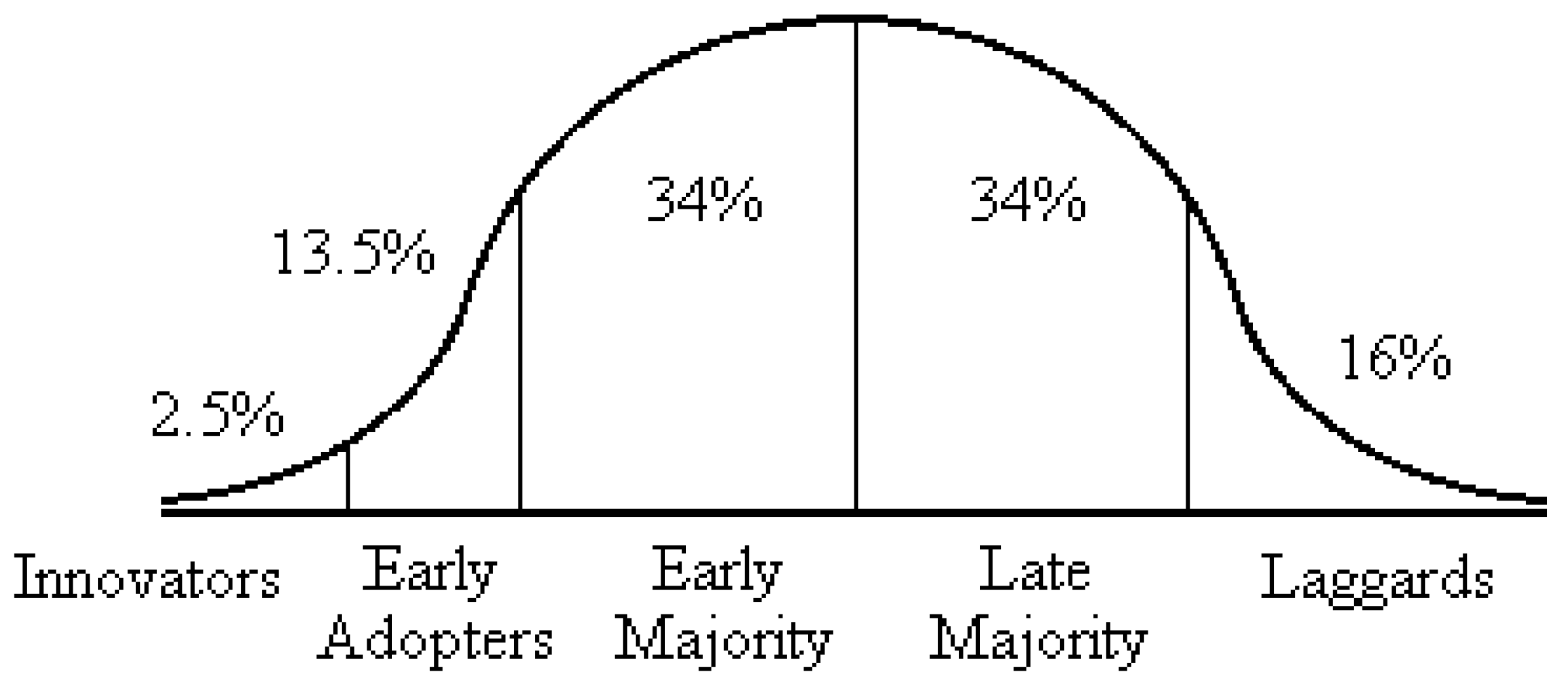
We begin our analysis by introducing the Rogers’ innovation diffusion curve [5] which can provide some ideas about patterns of homophily. As Figure 1 shows, there are five adopter categories named “innovators”, “early adopter”, “early majority”, “late majority” and “laggards”, respectively. According to Rogers, there is usually a normal distribution of the various adopter categories that forms the shape of a bell curve.

Figure 1. Rogers’ innovation diffusion curve.

Figure 1. Rogers’ innovation diffusion curve.

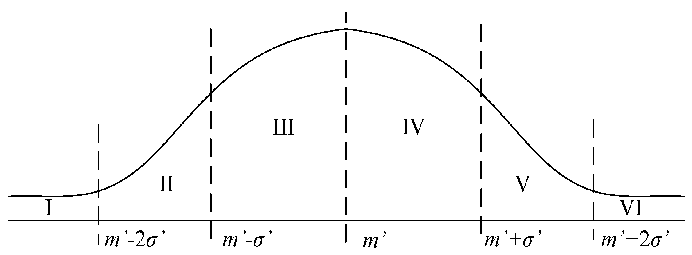
The Rogers’ adopter categories can be seen as a segregation of the population, so the five different behaviors about innovation adoption provide a pattern of homophily. Furthermore, we can find that the defined innovation value judgment variable a_i(0)s and the innovation adoption cost variable b_is both accord with the normal distribution as shown in Section 2.1.1. Similar to the Rogers’ idea, the above two kind of variables also can be segregated into six categories, as a result, two patterns of homophily can be defined accordingly.

Definition 1 (Homophily based on innovation value judgment, homophily_case_1 for short). Given the six categories as shown in Figure 2 where m’ represents the mean value and σ’ is the standard deviation, if a_i(t) and a_j(t) belong to the same category, then agents i and j are of homophily at the time t, otherwise, they are not of homophily.

Figure 2. The six categories.

Figure 2. The six categories.

Definition 2 (Homophily based on innovation adoption cost, homophily_case_2 for short). Given m and σ of variable b_is, if b_i and b_j belong to the same category, then agents i and j are of homophily, otherwise, they are not of homophily.

Obviously, the above two definitions are different. As for homophily_case_1, the homophily between the agents i and j is likely to change with system time going on, but as for homophily_case_2, it is not. The two cases represent two different kinds of homophily, the former one is not innate, that is to say, it can be formed or elapsed with the process of system evolution (e.g., before marriage, I am of homophily with other single people, but after I am married, the situation changes); the later one is innate like race, blood type and gender, and does not change in the system. Also, the two definitions of homophily accord with the idea of Rogers’ innovation diffusion curve to some extent.

Furthermore, we next introduce the concepts of “homophily index”, “relative homophily”, “baseline homophily”, “inbreeding homophily” and “heterophily” which have been defined by Currarini, et al. [13]. These concepts discuss the relationship between the relative fraction of type k in the population and the homophily index H_k defined as follows, which can take a closer look at homophily pattern and provide insights into innovation adoption.

Definition 3 (The relative fraction of type k in the population, denoted by w_k). Based on Figure 2 and the definition of homophily, all the population has been segregated into five categories. Let N_k denote the number of category k individuals in the population, where k = 1, 2,…, K. Then we define w_k as the relative fraction of type k in the population, which can be expressed as:

$$w_k=N_k/{\displaystyle {\sum }_{k=1}^K{N}_k}$$

(2)

Definition 5 (Homophily index, denoted by H_k). Let s_k denote the average number of agents who have links and are of the homophily with agents of type k, and d_k denote the average number of agents who have links and are not of the homophily with agents of type k. Then H_k is defined by:

$$H_k=s_k/(s_k+d_k)$$

(3)

Definition 6 (Relative homophily). A profile (s_k, d_k|k = 1, 2,…, K) satisfies relative homophily if w_i > w_j implies H_i > H_j.

Definition 7 (Baseline homophily, Inbreeding homophily, and Heterophily). A profile (s_k, d_k|k = 1, 2,…, K) satisfies baseline homophily if for all ks:

$$H_k=w_k$$

(4)

Or, it satisfies inbreeding homophily for type k if:

$$H_k>w_k$$

(5)

Or, it satisfies heterophily for type k if:

$$H_k<w_k$$

(6)

The above concepts will be applied to explore the behavior of innovation diffusion within a social network when homophily is considered. For more detailed information about definitions 3–7, one can refer to the paper done by Currarini, et al. [13].

2.1.3. Rules of Updating

Subsequently, the innovation value judgment of the agent i can be updated based on the above definitions about homophily. Let λ₁ be the information transferring index among the agents with homophily or in the same category and let λ₂ be the information transferring index among the agents without homophily or in the different categories. Then the rule of updating a_i(t) can be expressed as follows. There are four cases:

When s_i ≠ 0 and d_i ≠ 0:

$$a_i(t)=\frac{1}{2}\cdot \left(a_i(t-1)+\frac{{\lambda }_1}{{\lambda }_1+{\lambda }_2}\cdot \frac{{\displaystyle {\sum }_{j=1}^{s_i}{a}_j(t-1)}}{s_i}+\frac{{\lambda }_2}{{\lambda }_1+{\lambda }_2}\cdot \frac{{\displaystyle {\sum }_{j=1}^{d_i}{a}_j(t-1)}}{d_i}\right)$$

(7)

When s_i = 0 and d_i ≠ 0:

$$a_i(t)=\frac{{\lambda }_1+{\lambda }_2}{{\lambda }_1+2\cdot {\lambda }_2}\cdot \left(a_i(t-1)+\frac{{\lambda }_2}{{\lambda }_1+{\lambda }_2}\cdot \frac{{\displaystyle {\sum }_{j=1}^{d_i}{a}_j(t-1)}}{d_i}\right)$$

(8)

When d_i = 0 and s_i ≠ 0:

$$a_i(t)=\frac{{\lambda }_1+{\lambda }_2}{2\cdot {\lambda }_1+{\lambda }_2}\cdot \left(a_i(t-1)+\frac{{\lambda }_1}{{\lambda }_1+{\lambda }_2}\cdot \frac{{\displaystyle {\sum }_{j=1}^{s_i}{a}_j(t-1)}}{s_i}\right)$$

(9)

When d_i = 0 and s_i = 0:

$$a_i(t)=a_i(t-1)$$

(10)

where, s_i denotes the number of agents who have links and are of the homophily with the agent i, and d_i denotes the number of agents who have links and are not of the homophily with the agent i. In the above updating rules, λ₁ and λ₂ are exogenous, which is an assumption in the design of simulation analysis. Because we cannot find explicit factors in the system to affect or decide λ₁ and λ₂, we recognize them as exogenous variables. Accordingly, changing them and making comparisons become possible and desirable.

2.1.4. Network Structure

Four kinds of network topologies are often considered in the existing literature, which are the regular network, the random network, the small world network, and the power-law distribution network (or called the scale-free network). As for a regular network, a node can be defined to link with 2N neighbors, where N is an integer. Thus, such network has a constant number of edges for each of its nodes so that its diameter is rather large and proportional to its size. As for the random network, it was proposed by Erdös and Reyi [30], representing a large and complex network where each node is randomly connected with the others. The random network can be generated by connecting every pair of nodes with independent probability p. Unlike the regular network and the random network, the small world network possesses properties of both small diameter and high degree of clustering. The small network used in this paper was proposed by Watts and Strogatz [31], and it can be generated by rewiring each edge at random with a probability from a regular network with N nodes and k edges per node. Generally speaking, the small network is more similar to the real network than the above two kinds of networks. However, all the above three network topologies lack a hub characteristic of well-connected nodes. In fact, many real world networks exhibit the occurrence of highly connected nodes, such as the research citation network, the movie actor network, the World Wide Web, and so on. Barabási and Albert [32] proposed the power-law distribution network which can be generated by adding edges to the given nodes with a probability satisfying the power-law distribution.

2.1.5. Adoption Strategy

Every agent weighs its innovation value judgment [denoted by a_i(t)] and adoption cost (denoted by b_i) to decide whether to adopt the innovation or not. Thus, the adoption benefit of agent i at time t (denoted by c_i(t)) needs to be defined as follows:

$$c_i(t)=a_i(t)-b_i$$

(11)

We design two kinds of adoption strategies for these agents. Let d_i denote the adoption state of the agent i. The two kinds of adoption strategies are given through the following definitions:

Definition 8 (Strategy_case_1). If there exists t₀ making c_i(t₀) ≥ 0, then d_i = 1 and a_i(t) = a_i(t₀) for all t ≥ t₀. We call the agent i to be an innovation adoption agent.

Definition 9 (Strategy_case_2). Let t_∞ be the time when the dynamic system reaches its steady state, that is to say, all the a_i(t)s keep steady after the time t_∞. If c_i(t_∞) ≥ 0, then d_i = 1 and the agent i is an innovation adoption agent; Otherwise, d_i = 0 and the agent i is not an innovation adoption agent.

Strategy_case_1 shown in Definition 8 reflects the behavior of less than perfectly rational agents who makes decision only considering the current benefit. If an agent has adopted the innovation, we think the agent does not need to update its a_i(t), thus we assume that a_i(t) = a_i(t₀) for all t ≥ t₀, where t₀ is its adoption time. However, strategy_case_2 is used for depicting the perfectly rational agents who are able to make decisions according to the others’ responses and the final steady state of the dynamic system. The agents under strategy_case_2 have been updating their a_i(t)s until the system reaches its steady state. From the viewpoint of game theory, the decisions made by the agents under the strategy_case_2 reach Nash equilibrium, since no one has incentives to change its decision when the system reaches its steady state. Yet, some of the agents under strategy_case_1 are likely to regret their foregoing decisions because their benefits c_i(t)s are possible to be less than 0 if they consider the others’ responses and the final steady state of the dynamic system. The results caused by the two different kinds of strategies will be compared in the following simulation experiments.

2.2. Convergence Analysis

We make convergence analysis of the above simulation model in this part. First, we analyze the situation based on homophily_case_2, in which the updating process is a standard Markov process. To make it clear, we rewrite the updating rules in part 2.1.3 as follows:

$$a(t)=T\cdot a(t-1)$$

(12)

where, T is the state transition matrix and independent with time t. The elements of T are decided by Equations (7) to (10). Besides, the matrix T is a symmetric matrix in which the sum of each row or column equals 1. Also, a(t) is the vector consisting of a_i(t), i = 1,2,…,n.

According to the results on Markov chains [33], as long as the network is connected, the process will convergence to a limit, which is summarized to the following Theorem 1 [29]:

Theorem 1. If the network is connected, then T^t convergences to a limit T^∞ such that

$${(T^{\infty })}_{ij}={\displaystyle {\sum }_{i=1}^n{(T)}_{ij}}/{\displaystyle {\sum }_{i,j=1}^n{(T)}_{ij}}$$

(13)

Theorem 1 implies that the updating process is convergent, and for any initial vector, all agents’ beliefs converge to a consensus. It is noted that the above theorem is just suitable for the situation based on homophily_case_2.

The next question is in what conditions the network is connected. It is clear that the regular network and scale free network are connected because of their generating rules. For the WS small world network, it is possible for it to be a unconnected one, but the probability is much lower than the random network under the same number of nodes and average degree of per node. Thus, the core is to discuss in what conditions the random network is connected. Fortunately, Bollobás has given the answer to the above question in his book [34].

Theorem 2. The probability equals one that a random network is connected if the probability of linkage between nodes is more than ln(N)/N. Where, N is the number of nodes. In fact, the above condition is equivalent that the average degree of per node denoted by q is larger than (N-1)ln(N)/N.

Proof of the second part. The first part of theorem can be found in [34], let us prove the second part.

It is obvious that given the average degree of per node denoted by q, the linkage probability of such a random network denoted by p is:

$$p=\frac{q\cdot N/2}{N\cdot (N-1)/2}$$

(14)

Accordingly, the inequality p > (lnN)/N can be rewritten as:

$$q>\frac{N-1}{N}\ln (N)$$

(15)

So, the second part holds.

According to the Theorem 2, if q is larger than lnN, the four kinds of network will all be connected. It is noted that the above Theorem 2 only gives a sufficient condition. Accordingly, we do not make q larger than lnN in the following simulation analysis, which is for two reasons: (1) the situation of q larger than (lnN)/N has been studied sufficiently since it has had analytical solutions (see also Golub and Jackson [29]); (2) Even if q is not larger than (lnN)/N, the updating process in the context of random network may also be convergent. As a result, we make N as 500 and q as 4 in the following simulation analysis, where 4 is smaller than ln (500).

However, for the situation based on homophily_case_1, the state transition matrix T shown in Formula (12) changes with time t, because the matrix is the function of a(t) and the a(t) changes with time going on. As a result, it does not satisfy the conditions of standard Markov process and the theorem 1 is not suitable. Thus, the agent-based simulation is necessary since the existed theorems cannot give the answer of such questions.

2.3. Simulation Steps

The whole simulation steps can be summarized on the basis of the above definitions and statements. The five steps are listed as follows:

Step 1. Set the value of m and σ shown in Formula (1). By the way, by changing m and σ, it can be reflected that how the state of the dynamic system depends on its initial values.

Step 2. Choose the definition of homophily from Homophily_case_1 or Homophily_case_2 which have been stated in section 2.1.2, and set the values of λ₁ and λ₂. It is noted that the different definitions of homophily and the different values of λ₁ and λ₂ will decide the rule of updating so that the state of dynamic system will be affected accordingly.

Step 3. Giving the number of nodes (N) and the average degree of per node (q), we generate the four kinds of networks and examine how their topologies affect the adoption behavior.

Step 4. Choose Strategy_case_1 or Strategy_case_2 as the strategy of the system, and compare them to uncover how the strategy affects the adoption rate and the adoption time.

Step 5. Decide the rule that the system is terminated and then do simulation 100 times and average the result. Output the adoption rate, the adoption time, or other defined indexes in the following section. Compare them to explore the characteristics of innovation adoption in social networks with different features.

3. Simulation Results

In this section, we will explore the characteristics of innovation adoption based on the agent-based model established as above. In each subsection, we will introduce the parameters of the system and their values firstly, and then point out that which variable is the control one. In the last part of each subsection, the findings will be summarized.

3.1. Initial Value and Its Influences

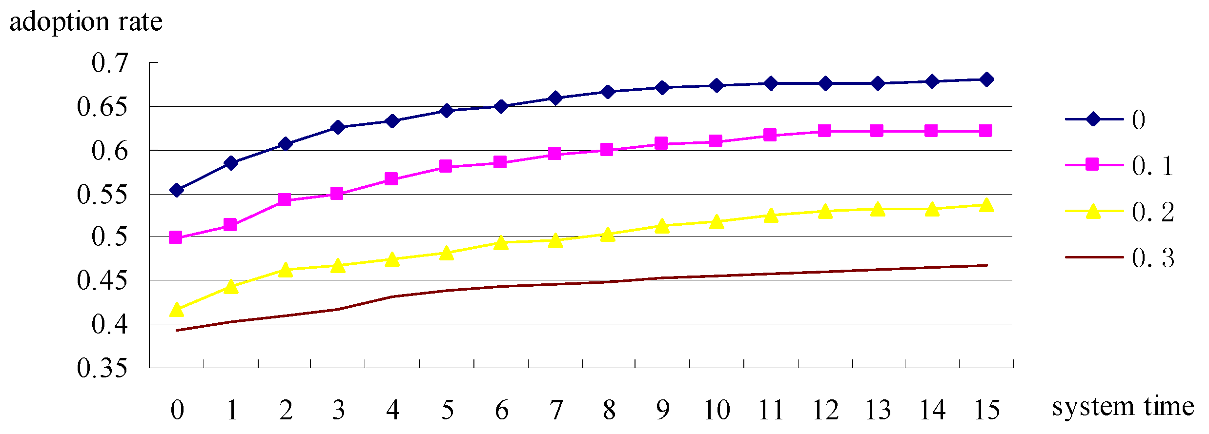
Let N = 500, q = 4, λ₁ = 0.8 and λ₂ = 0.2. The system adopts strategy_case_1 and homophily_case_1, and applies the small-world network as its topology (In fact, the other topologies show the similar feature). Here, the mean value m of b_is changes from 0 to 0.3 by 0.1 each time. The following four curves shown in Figure 3 are corresponding to the four values of m, respectively.

Figure 3. System time-adoption rate curve under different mean values.

Figure 3. System time-adoption rate curve under different mean values.

As Figure 3 shows, different mean values of adoption cost (b_is) cause different initial adoption rates and different steady-state adoption rates. Furthermore, the mean value does not affect the adoption time of the system significantly. All these can be summarized to be the statement: In this model, when the adoption cost rises, the corresponding initial adoption rate and the steady-state adoption rate will decease and vice versa. Besides, the mean value of the adoption cost does not affect the adoption time significantly.

The above statement may be straightforward, since the dynamics of the system are described fully by a_is and not affected by b_is under strategy_case_1 and homophily_case_1. However, the specific adoption rate and the adoption time cannot be given just based on the above analysis; especially the analytical solution is difficult to be obtained under the setup of strategy_case_1 and homophily_case_1. Thus, the above statement also provides the numeric results of the adoption rate and the adoption time, which may give a benchmark for further studies.

3.2. Homophily and Its Influences

Let b_is be independent for all i and satisfy N(0,1), N = 500, q = 4, λ₁ = 0.8 and λ₂ = 0.2. The system adopts the strategy_case_1. Following the simulation steps, we compare the adoption rate and adoption time caused by the two homophily cases. Recall that the homophily_case_1 is defined based on the homophily of a_i(t)s, and the homophily_case_2 based on b_is. Table 1 shows the results as follows.

From Table 1, we can find that the adoption rate and the adoption time under the homophily_case_1 are both smaller than the corresponding part under the homophily_case_2, no matter what network topology is adopted. In fact, b_is are exogenous variables of the system, which means they do not change with the evolvement of the system. Using such variables to define the homophily, we find that it can bring the diversity into the system.

Table 1. Adoption rate and adoption time under the two homophily cases.

Items	Homophily case	Regular network	Random network	Small-world network	Scale-free network
adoption rate	homophily_case_1	0.6352	0.6237	0.6208	0.6215
	homophily_case_2	0.6397	0.6266	0.6287	0.6274
adoption time	homophily_case_1	37.10	39.85	30.45	32.55
	homophily_case_2	58.55	40.20	31.15	48.70

Table 1. Adoption rate and adoption time under the two homophily cases.

Items	Homophily case	Regular network	Random network	Small-world network	Scale-free network
adoption rate	homophily_case_1	0.6352	0.6237	0.6208	0.6215
	homophily_case_2	0.6397	0.6266	0.6287	0.6274
adoption time	homophily_case_1	37.10	39.85	30.45	32.55
	homophily_case_2	58.55	40.20	31.15	48.70

As a result, it cause a higher adoption rate, but a larger adoption time than the case of using the endogenous variables (a_i(t)s) to define the homophily. Thus, we obtain the following finding:

Finding 1: In this model, using exogenous variables to define the homophily can cause a higher adoption rate and larger adoption time than using endogenous variables, no matter what network structure is adopted.

The “system time-adoption rate” curve shown in Figure 3 reminds us that the adoption time of each agent also can be a source of homophily. Thus, we can divide all the agents into five categories denoted by k = 1,2,…,5 respectively, and the corresponding time intervals from left to right are 0, (1, 0.15 t_∞], (0.15 t_∞, 0.50 t_∞], (0.50 t_∞, t_∞], (t_∞, ∞), where t_∞ is the time when the innovation adoption system reaches its equilibrium. When the homophily_case_1 is adopted and the other initial conditions are the same in this subsection, the results are listed in the following Table 2.

Table 2. The values of w and H.

Network topology	w and H	k = 1	k = 2	k = 3	k = 4	k = 5
regular network	w	0.4449	0.0667	0.0472	0.0022	0.4390
	H	0.4521	0.0097	0.0080	0.0000	0.2112
random network	w	0.4484	0.0649	0.0451	0.0032	0.4384
	H	0.5315	0.0082	0.0111	0.0004	0.2425
small-world network	w	0.4550	0.0482	0.0628	0.0070	0.4270
	H	0.4701	0.0044	0.0095	0.0001	0.2012
scale-free network	w	0.4386	0.0434	0.0603	0.0096	0.4481
	H	0.4537	0.0032	0.0104	0.0004	0.2304

Table 2. The values of w and H.

Network topology	w and H	k = 1	k = 2	k = 3	k = 4	k = 5
regular network	w	0.4449	0.0667	0.0472	0.0022	0.4390
	H	0.4521	0.0097	0.0080	0.0000	0.2112
random network	w	0.4484	0.0649	0.0451	0.0032	0.4384
	H	0.5315	0.0082	0.0111	0.0004	0.2425
small-world network	w	0.4550	0.0482	0.0628	0.0070	0.4270
	H	0.4701	0.0044	0.0095	0.0001	0.2012
scale-free network	w	0.4386	0.0434	0.0603	0.0096	0.4481
	H	0.4537	0.0032	0.0104	0.0004	0.2304

According to the Definition 6 (relative homophily) given in section 2.1.2 of this paper, the homophily defined by the system time satisfies the conditions of relative homophily. Besides, according to the Definition 7 of this paper, the category k = 1 satisfies the inbreeding homophily slightly, while the other four categories satisfy the definition of heterophily. The above laws are independent with the network structure. The reasons for this are complex, but one thing is certain that the behavior of adoption is affected by many factors including the links generated by homophily but not restricted to it.

Finding 2: The homophily defined by the system time satisfies the relative homophily. The category k = 1 (or the so-called the “innovators” following the definition from Rogers) reflects the feature of inbreeding homophily, while the other categories satisfy the definition of heterophily.

3.3. Updating Rule and Its Influence

Let N = 500 and q = 4. The system adopts the strategy_case_1 and applies the small-world network as its topology. We change the λ₁ from 0.55 to 0.95 by 0.05 each time, and the corresponding λ₂ changes from 0.45 to 0.05 by 0.05 each time. It is noted that we keep λ₁ + λ₂ = 1 and the total number of pairs (λ₁, λ₂) is 9. The system is designed to stop when the system time equals 15, in which time all the cases are near to their steady states but have not reached them. We choose the stop time as 15 for two reasons. First, in the real world, the innovation adoption time is not unlimited, often the innovation has its own lifecycle, and thus setting the stop time is reasonable. Second, if all the agents in some cases have finished their adoptions while others not, it is unfair to compare them because the unfinished agents can still update their adoption decisions while the finished cannot.

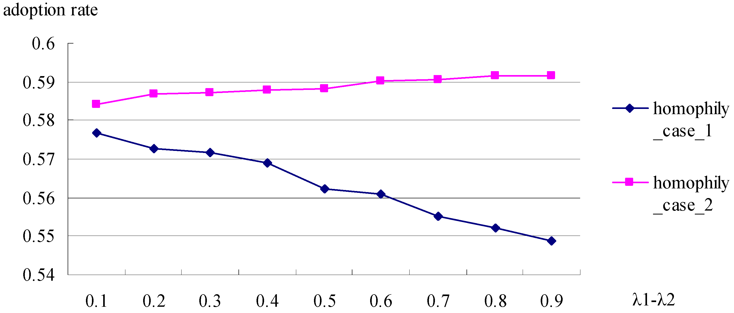
Recall that λ₁ is the information transferring index among the agents in the same category, and λ₂ is that in the different categories. Often λ₁ > λ₂, and the more the value of λ₁-λ₂ is, the bigger the gap of the information transferring ability in two cases is.

As Figure 4 shows, when homophily_case_1 is adopted, the increasing λ₁-λ₂ causes the decreasing adoption rate. The reason for the fact is that a_i(t)s are used not only for deciding homophily, but also for updating in the homophily_case_1, so that the increasing λ₁-λ₂ means too fast learning within the same categories and excluding the information from outside, which blocks the innovation diffusion between categories. While, when b_is are used for deciding homophily and a_i(t)s are used for updating, the situation is not the same, since the increasing λ₁-λ₂ increases the speed of learning and causes an increasing adoption rate.

Figure 4. Adoption rate at different values of λ₁-λ₂ under two cases of homophily.

Figure 4. Adoption rate at different values of λ₁-λ₂ under two cases of homophily.

Finding 3: The effect of increasing λ₁-λ₂ depends on what variables are used for deciding these categories. If the variable is also used for updating, the adoption rate will decrease because the too fast learning within the same categories will exclude the information from outside. While, if the variables is exogenous or not used for updating, the adoption rate will rise gradually because the increasing λ₁-λ₂ boosts the speed of learning.

3.4. Network Topology and Its Influence

From Table 1 and Table 3 below, the small-world network has the shortest adoption time compared to the other three. Next to the small-world network is the scale-free network, and the latter two are random network and regular network in terms of adoption time. The phenomenon indicates that the small-world network has the strongest ability of innovation diffusion. The finding is very common and many literatures have found it such as [1] and [10].

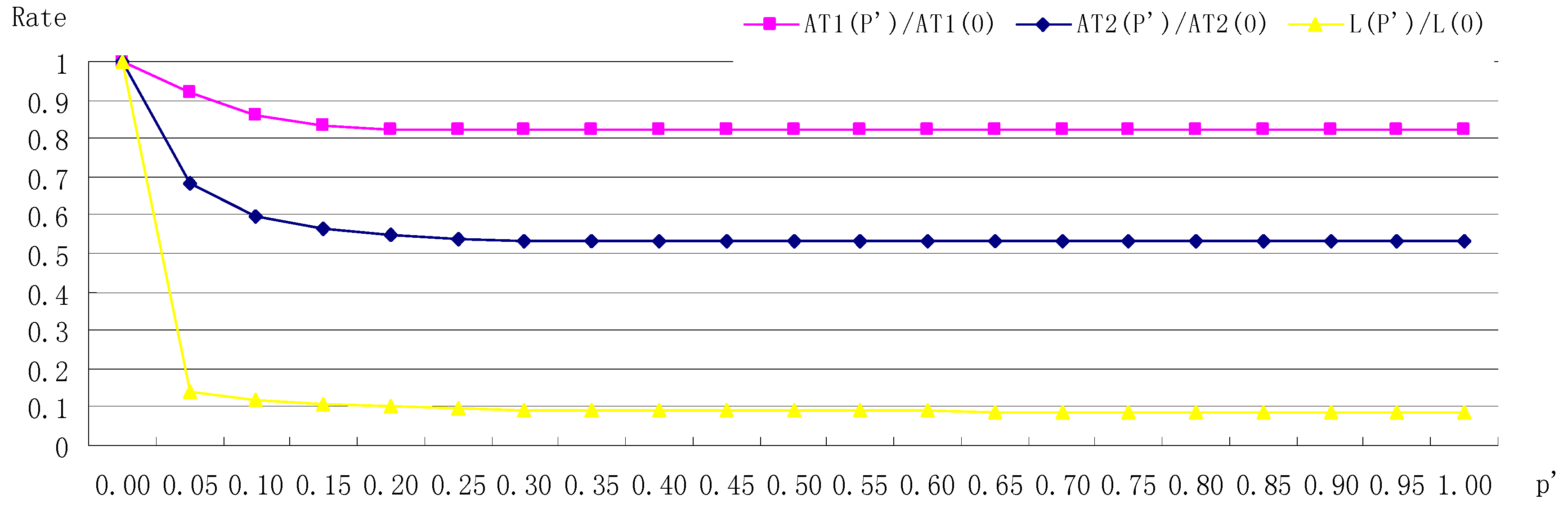
Besides, in the context of small-world network, let the rewriting probability denoted by p’ change from 0 to 1 by 0.05 each step. Then we further make N = 500, q = 4, λ₁ = 0.8 and λ₂ = 0.2. The two series of adoption time at different values of p’ can be obtained based on the two cases of homophily respectively. To make the comparisons clear, we use p’-rate graph to show the results, in which AT₁(p’) epresses the adoption time under homophily_case_1 at rewriting probability p’, AT₂(p’) expresses the one under homophily_case_2, and L(p’) expresses the average path length of the network at p’. Accordingly, the rate values of AT₁(p’)/AT₁(0), AT₂(p’)/AT₂(0) and L(p’)/L(0) at different values of p’ are shown in Figure 5 as follows.

Figure 5. Adoption time and average path length at different values of $p\prime$ in the context of small-world network.

Figure 5. Adoption time and average path length at different values of $p\prime$ in the context of small-world network.

Table 3. Adoption rate and adoption time under the two strategy cases.

Items	Strategy case	Regular network	Random network	Small-world network	Scale-free network
adoption rate	strategy_case_1	0.6352	0.6237	0.6208	0.6215
	strategy_case_2	0.5051	0.4973	0.4955	0.4840
adoption time	strategy_case_1	37.10	39.85	30.45	32.55
	strategy_case_2	129.55	75.10	37.90	40.00

Table 3. Adoption rate and adoption time under the two strategy cases.

Items	Strategy case	Regular network	Random network	Small-world network	Scale-free network
adoption rate	strategy_case_1	0.6352	0.6237	0.6208	0.6215
	strategy_case_2	0.5051	0.4973	0.4955	0.4840
adoption time	strategy_case_1	37.10	39.85	30.45	32.55
	strategy_case_2	129.55	75.10	37.90	40.00

From Figure 5, we can find that the shorter the average path length is, the less the adoption time is, no matter what the definition of homophily is adopted. Thus, the adoption time is highly correlated with the average distance in the small-world.

Finding 4: The small-world network has the shortest adoption time compared to the other three, which means that the small-world network has the strongest ability of innovation diffusion. Besides, the adoption time is correlated with the average distance in the small-world network, and the shorter the average distance is, the less the adoption time is.

3.5. Strategy and Its Influences

Let b_is be independent for all is and satisfy N(0,1), N = 500, q = 4, λ₁ = 0.8 and λ₂ = 0.2. The system adopts the homophily_ case_1. Then the results of comparing the two strategy cases are listed below.

Compared to strategy_case_1, the agents under strategy_case_2 are more intelligent. The clever agents are able to know others’ decisions and react to them, as a result, they share a lower adoption rate because they cannot make a mistake and regret themselves, but they also need more time to reach the equilibrium of their gaming in the system. From Table 3, we can obtain the following finding.

Finding 5: If the agents in the system are myopic, the system will have a higher innovation adoption rate and shorter adoption time. While, if the agents can grasp all the information and react to others’ decisions, the innovation diffusion will face some resistance, to some extent.

4. Conclusions

We have constructed a new agent-based model to explore the characteristics of innovation adoption in the context of social network. We give detailed discussions and definitions about the network structure, homophily, and decision-making strategy. Especially, we consider the effects from the homophily, which is a new topic in the field of innovation adoption. In the simulation experiments, we examine five aspects and their influences on the behavior of agents’ innovation adoption, and the five aspects are initial conditions, homophily, network topology, rules of updating and strategy, respectively. These results from the above simulation experiments obtain seven pieces of findings as follows: (1) the initial conditions affect the behavior of innovation adoption, specifically, the mean value of adoption cost affects the adoption rate, but does not affect the adoption time significantly; (2) using exogenous variables to define the homophily can cause a higher adoption rate and larger adoption time than using endogenous variables, no matter what network structure is adopted; (3) The homophily defined from different sources can cause different results, especially, the homophily defined by system time satisfies the relative homophily; (4) The effect of learning efficiency depends on what variables are used for deciding these agents’ categories; (5) the small-world network has the strongest ability of innovation diffusion; (6) the adoption time is highly correlated with the average distance in the small-world network; (7) If the agents in the system are short-sighted, the system will have a higher innovation adoption rate and shorter adoption time. While, if the agents can grasp all the information and react to others’ decisions, the innovation diffusion will face some resistance, to some extent. Based on the above findings, if we want to boost the innovation adoption, we should try to decrease the adoption cost, or enrich the links among these agents, especially enhance the homophily obtained from endogenous variables of this system, or encourage the agents to make them brave and not to care the others’ decisions too much.

However, the model presented here assumes that all the agents have an identical strategy and updating rule, but this assumption is not common in real life. We may make several kinds of agents so that they can react differently. If so, we guess the behaviors of innovation adoption in the system will become more complex, and this may provide more important findings and management advice.