Multiscale Interactions betweenWater and Carbon Fluxes and Environmental Variables in A Central U.S. Grassland

Abstract

The temporal interactions between water and carbon cycling and the controlling environmental variables are investigated using wavelets and information theory. We used 3.5 years of eddy covariance station observations from an abandoned agricultural field in the central U.S. Time-series of the entropy of water and carbon fluxes exhibit pronounced annual cycles, primarily explained by the modulation of the diurnal flux amplitude by other variables, such as the net radiation. Entropies of soil moisture and precipitation show almost no annual cycle, but the data were collected during above average precipitation years, which limits the role of moisture stress on the resultant fluxes. We also investigated the information contribution to resultant fluxes from selected environmental variables as a function of time-scale using relative entropy. The relative entropy of latent heat flux and ecosystem respiration show that the radiation terms contribute the most information to these fluxes at scales up to the diurnal scale. Vapor pressure deficit and air temperature contribute to the most information for the gross primary productivity and net ecosystem exchange at the daily time-scale. The relative entropy between the fluxes and soil moisture illustrates that soil moisture contributes information at approximately weekly time-scales, while the relative entropy with precipitation contributes information predominantly at the monthly time-scale. The use of information theory metrics is a relatively new technique for assessing biosphere-atmosphere interactions, and this study illustrates the utility of the approach for assessing the dominant time-scales of these interactions.

1. Introduction

The transfer of water between the terrestrial surface and the atmosphere can account for large portions of the available energy. If this flux is transferred from the soil moisture pool to the atmosphere via vegetation, then this flux of water becomes intricately tied to the assimilation of carbon. Understanding the biophysical mechanisms that control the interactions between the water and carbon cycles between the land surface and the atmosphere is vitally important for monitoring and predicting the responses of these environments under global climate change.

The interactions between driving factors that govern the coupling of carbon and water fluxes in natural conditions are poorly understood [1]. Ultimately, this is an issue involving scales ranging from the micrometer scale of stomatal pores up to the scale of the largest eddies within the atmospheric boundary layer (on the order of kilometers). One of the best tools to decompose a signal across spatial and/or temporal scales is wavelet-based multiresolution analysis. Wavelet transforms have been used to characterize the dominant temporal scales of land surface fluxes [2], the relative control of various meteorological variables on the ecosystem responses [3,4], the interaction between local fluxes and regional circulations, like monsoonal patterns [5], and to provide a quantitative comparison of these interactions across ecosystems [6]. Such diagnostics of the cross scale variability of fluxes between the surface and the atmosphere can help evaluate current models [7,8].

The nature of the scale interactions raises important issues for understanding the biophysical dynamics; in particular, the role of optimization within vegetation to maximize carbon gain while minimizing water loss [9]. Understanding the nature of the interactions between the water and carbon cycle is particularly important in grasslands for agricultural and other reasons. Grassland ecosystems account for a significant portion of the land surface, and climate change could have a significant impact on their ecology and functioning [10,11]. These ecosystems may have the potential for acting as a global carbon sink more than is normally realized [12]. Therefore, quantifying how this potential will change in response to global and regional climate changes necessitates an understanding of phenological responses [13], as well as microscale impacts, such as light and water use [14].

Productivity in grassland ecosystems is extremely sensitive to the timing and magnitude of precipitation events, which modulate the water use efficiency [15,16,17]. This mechanism is tightly coupled to the available soil moisture [18] and the interannual variability in rainfall [19,20]. Variability in precipitation and soil moisture leads to alterations of the carbon flux via the water use efficiency [14,21], which has led to the examination of the role of optimal water use, particularly during drought conditions [22,23,24,25].

Eddy covariance measurements have been widely used to evaluate the interactions between carbon and water fluxes, as well as their relationships with local environmental factors, such as radiation, humidity, soil moisture, etc. Although eddy covariance is characterized by the inability to close the energy balance on many sites, (including grasslands [26]), and this is problematic for the monitoring of water and carbon cycling [27], the technique is nonetheless helpful for assessing carbon and water fluxes and the relationships with the local environmental variables. In grasslands that exhibit both $C_3$ and $C_4$ species, water limitation plays an important role in governing canopy scale water and carbon fluxes [28,29], but species composition may also exhibit some control over the their coupling [30].

Given the potential importance of changes in land-atmosphere fluxes of carbon and water and regional climate [31,32], it is important to explore the temporal scales of water and carbon fluxes and their interactions with environmental factors. In this study, we examine these processes in a mixed $C_3$-$C_4$ grassland experiencing woody succession—a land use representative of a significant fraction of Midwestern North America. Specifically, we examine the role of different time-scales on water and carbon fluxes, and the relationship between fluxes and environmental factors as a function of time-scale.

2. Methods

2.1. Site Description

Data was collected at the Kansas Field Station (KFS) Ameriflux station (39${}^{\circ }$N, 94${}^{\circ }$W) [33]. This is an abandoned grassland, operated by the University of Kansas Ecological Reserve. The region exhibits a mean annual temperature of 13.3 ${}^{\circ }$C and mean annual precipitation of 937 mm. Soils are classified as fine, montmorillonitic, mesic aquic argiudolls.

The site was subjected to intensive agriculture during the 1940s to the 1960s. In the mid-1970s, the site was planted with the cool-season grass Bromus inermis and used as a hay meadow until 1987. Mowing and burning approximately every five years has maintained it as a grassland until the present. The site was most recently burned on April 1, 2009. Vegetation species at the site consists of Bromus inermis, Festuca arundinacea, and Poa pratensis grasses, as well as a native grass, Andropogon virginicus, and several native forbs.

2.2. Field Measurements and Processing

Water and carbon fluxes were measured using the eddy covariance technique from day of year (DOY) 166, 2007 to DOY 365, 2010. Turbulent fluctuations of temperature and wind speeds were measured using a 3D sonic anemometer (CSAT-3, Campbell Scientific, Logan, UT USA), and water vapor and carbon dioxide were measured using an open path infrared gas analyzer (LI-7500, Li-Cor, Lincoln, NE, USA) at a temporal resolution of 20 Hz. The Li-7500 was inclined to 15${}^{\circ }$ into the mean wind direction.

In addition to the flux measurements of latent heat ($LE$), sensible heat and net ecosystem exchange of carbon ($NEE$), a standard suite of microclimatic variables, was also measured. Net radiation ($Rn$) was measured using a REBS Q7. The net radiometer suffered bird damage and was inoperative from October 15 until November 14, 2007. The Q7 was replaced with a Kipp & Zonen four-way radiometer on November 30, 2009. Photosynthetic photon flux density (PPFD) was measured using a Li-Cor LI-190SA at 1.5 m above the surface on a separate mast mounted close to the eddy covariance measurements. An additional anemometer (Campbell Scientific 014A Met One sensor) was mounted with the net radiometer to correct the net radiation values to account for air flow and heat storage. Soil heat flux (G) was measured using two HFT-3 (Campbell Scientific) plates at 8 cm and was corrected for heat storage above the plate using soil temperature measurements at 2 and 5 cm. Volumetric soil moisture was measured using a Frequency Domain Reflectometry sensor of type ML2x theta probe (Delta-T Devices) at 8 cm. Air temperature ($T_a$) and humidity were also measured using an HMP-45 sensor. Precipitation ($PPT$) was measured using a Texas Instruments tipping bucket rain gauge. The precipitation gauge suffered damage in July–August 2010, and data for that period was replaced with observations from a SCAN site located approximately 1 km south of the tower. All ancillary measurements were averaged over 30 min intervals and stored on a Campbell Scientific CR3000. All years were marked by higher than average precipitation at the site.

The 20 Hz time series of turbulent measurements were processed using a combination of Edi-Re (version 1.4.3.1167, R. Clement, University of Edinburgh, UK) and R code (www.r-project.org). Half hour fluxes were determined from the covariance between fluctuations in vertical wind speed ($w^{\prime }$) and the associated scalar (temperature, $T^{\prime }$, carbon, $c^{\prime }$, and water vapor, $q^{\prime }$) by:

$$F_x=\overline{w^{\prime }{x}^{\prime }}$$

(1)

where $F_x$ is the vertical flux associated with scalar x, and the overbar signifies the temporal average. The calculations involved applying a planar fit coordinate rotation [34], as well as corrections for fluctuations in air density according to [35].

Quality control was conducted using the integral turbulence characteristics and stationarity tests [36]. The integral turbulence test compares the ratio of the standard deviation of vertical wind speed to the friction velocity (${\sigma }_w/u_{*}$) to the theoretical value. Here, any value greater than $30\%$ was removed. For the stationarity test, any six intervals differing by more than $60\%$ were neglected.

The net ecosystem exchange is partitioned into gross primary productivity ($GPP$) and ecosystem respiration ($RE$) using (author?) [37] by fitting a non-linear least squares regression between soil temperature and the nighttime eddy covariance observations with a $u_{*}$ value of greater than 0.15. This constraint of the higher turbulence nighttime conditions resulted in 57% of the nighttime data being available for the respiration calculation. This function is then applied to all eddy covariance $NEE$ observations to estimate the $GPP$ flux, which is calculated as $GPP=NEE-RE$.

Carbon and water flux values were filtered based on reasonable values, which included $120\%$ of Priestly-Taylor potential evapotranspiration ($PET$) for the latent heat flux ($LE$) and a linear interpolation of seasonal variation in the carbon flux. Gap filling of fluxes was performed following the methodology of [38] making use of the observed meteorological data of air temperature ($T_a$), vapor pressure deficit ($VPD=e_s-e_a$, were e is the vapor pressure at either saturation, s, or the actual, a, observed value) and the solar radiation ($R_g$), using a 7 day or a 15 day diurnal mean window. If the meteorological data were not available, we filled it using solar radiation if it was still available. If none of the values were available, a mean diurnal pattern was calculated from a short window (beginning at 1 day) and progressively widening until no missing values were present.

One possible area of concern may be the role of the gap filling algorithm on the determination of the scalewise variations. To examine this, we conducted the analysis for both the gap filled and non-gap-filled data. While there were some minor differences between the two cases, the overall behavior was not altered by the use of the gap-filled data. Therefore, we focus solely on the gap filled data analysis in this study.

2.3. Multiscale Information Theory Metrics

The time=scales of variability in the carbon and water fluxes are assessed using a wavelet multi-resolution analysis. Wavelets provide an excellent analysis technique for assessing the variability of temporal and spatial data across scale [39]. The wavelet transform ($W(m,n)$) was conducted using the Daubechies least-symmetric 8 wavelet as the mother wavelet (ψ), which provides a good balance between local support in both the frequency and temporal domains. The mother wavelet is then translated (n) and dilated (m) across a time-series f as a function of time t:

$$W(m,n)={\lambda }_0^{-m/2}{\int }_{-\infty }^{\infty }f\left(t\right)\psi \left({\lambda }_0^{-m}t-n{t}_0\right)dt$$

(2)

where ${\lambda }_0$ is the initial time-scale. The wavelet is given by:

$${\psi }_{m,n}\left(t\right)=\frac{1}{\sqrt{{\lambda }_0^m}}\psi \left(\frac{t-n{t}_0{\lambda }_0^m}{{\lambda }_0^m}\right)$$

(3)

The multi-resolution analysis consists of using the wavelet transform to compute band-pass filtered versions of the time-series at each time-scale of interest (m). The original time series ($f\left(t\right)$) can be reconstructed from the inverse wavelet transform by summing all of the reconstructions at each scale, m:

$$f\left(t\right)=\overline{f_m\left(t\right)}+\sum _{m\ge m_0}{f}_m^{\prime }\left(t\right)$$

(4)

We are interested in quantifying the variation of the water and carbon fluxes across time-scales, as well as the relationship with environmental variables as a function of time-scale. For these purposes, we use the decomposed time series at each scale ($f_m^{\prime }$) as input to the information theory metrics.

The first information theory metric of interest is the Shannon entropy (H). This is a measure of the information content of a data set. It is a stochastic measure based on the probability density function (PDF), and quantifies the statistical uncertainty within the PDF:

$$H\left(x\right)=-\sum _{i=1}^{n}p\left(x_i\right)log\left(p\left(x_i\right)\right)$$

(5)

where $p\left(x_i\right)$ is the probability of variable, x, within some small interval, i, of the probability density function. We estimated the probability density of function using the density command in the R software package, and this discrete estimate is then used as the probability.

The relative entropy ($R(x,y)$) is a measure of the distance between the PDFs (p and q) of two variables (x and y) [40]. This is a measure of the additional information necessary to characterize p from the information contained within q. Thus, the more information provided about p from q, the smaller the relative entropy and the less additional information is necessary to characterize the distribution of x given by p. The relative entropy is computed as:

$$R(x,y)=\sum _i{p}_{i}log\left(\frac{p_i}{q_i}\right)$$

(6)

We computed the relative entropy for two different purposes. In the first case, we computed the relative entropy between each scale of the multi-resolution analysis and the original data. This was done to quantify the amount of information that is contributed from each time-scale. In the second analysis, we computed the relative entropy between each scale of the environmental factors (from the wavelet decomposition) and the flux data to assess how much information about the flux could be inferred from the environmental variables for various time-scales.

To compute the entropy of the fluxes and environmental variables, we first decomposed the time series using the wavelet multiresolution analysis described above. At each scale of decomposition, the PDF of the decomposed time series ($f_m^{\prime }\left(t\right)$) was estimated and used to compute the Shannon entropy and relative entropy as a function of time-scale of decomposition.

We are not interpreting the entropy and relative entropy as indicators of predictability. We are interested in using these measures as a descriptive metric of the variability of the statistical distributions across time-scales, as well as the information loss between the distributions of environmental variables and the fluxes. We are specifically not addressing issues related to the independence of the various samples within the distributions, etc. Rather, we are attempting to use these metrics to look at the variability across time-scales in order to infer time-scales of strong interactions and time-scales of relatively weak interactions.

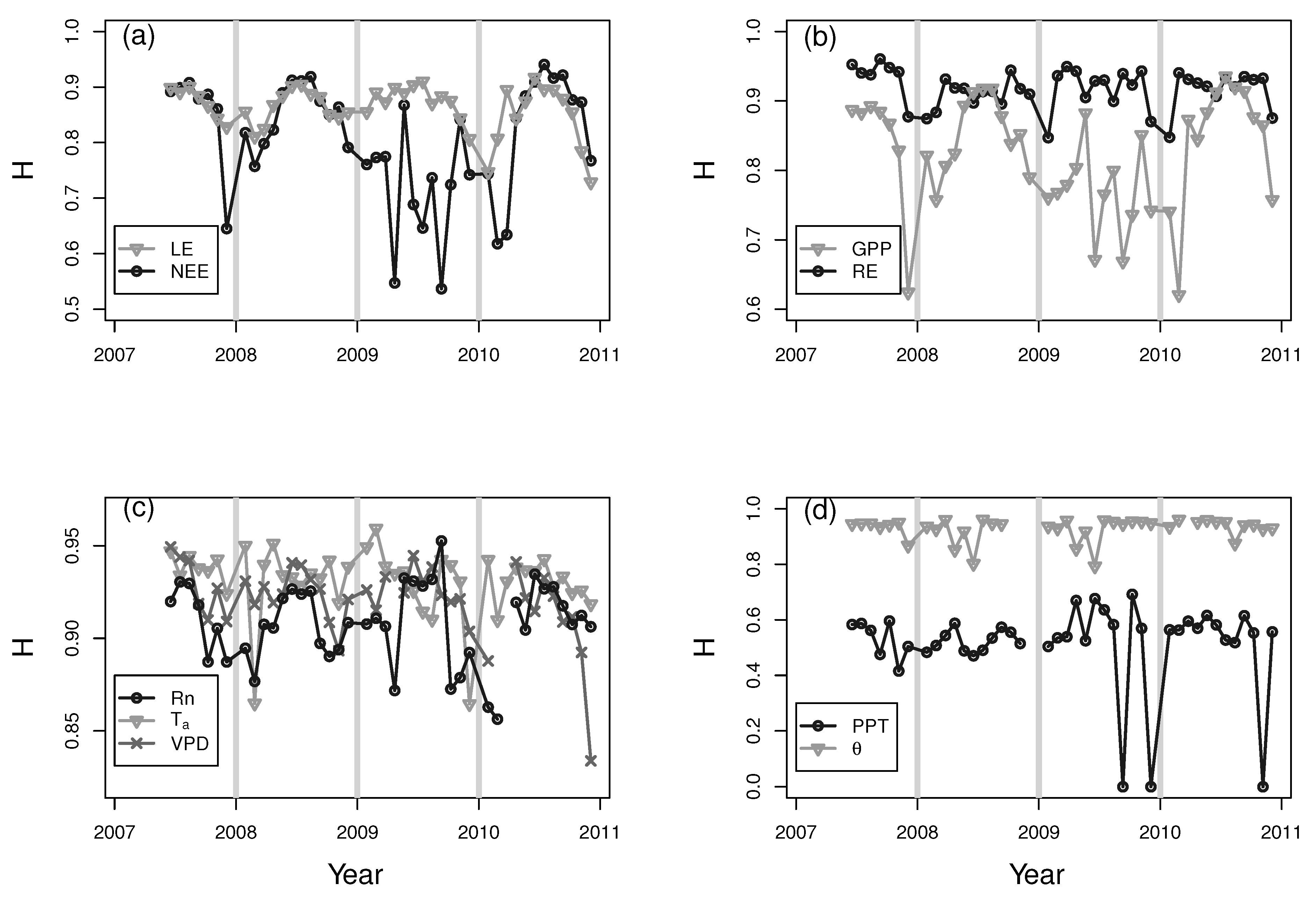
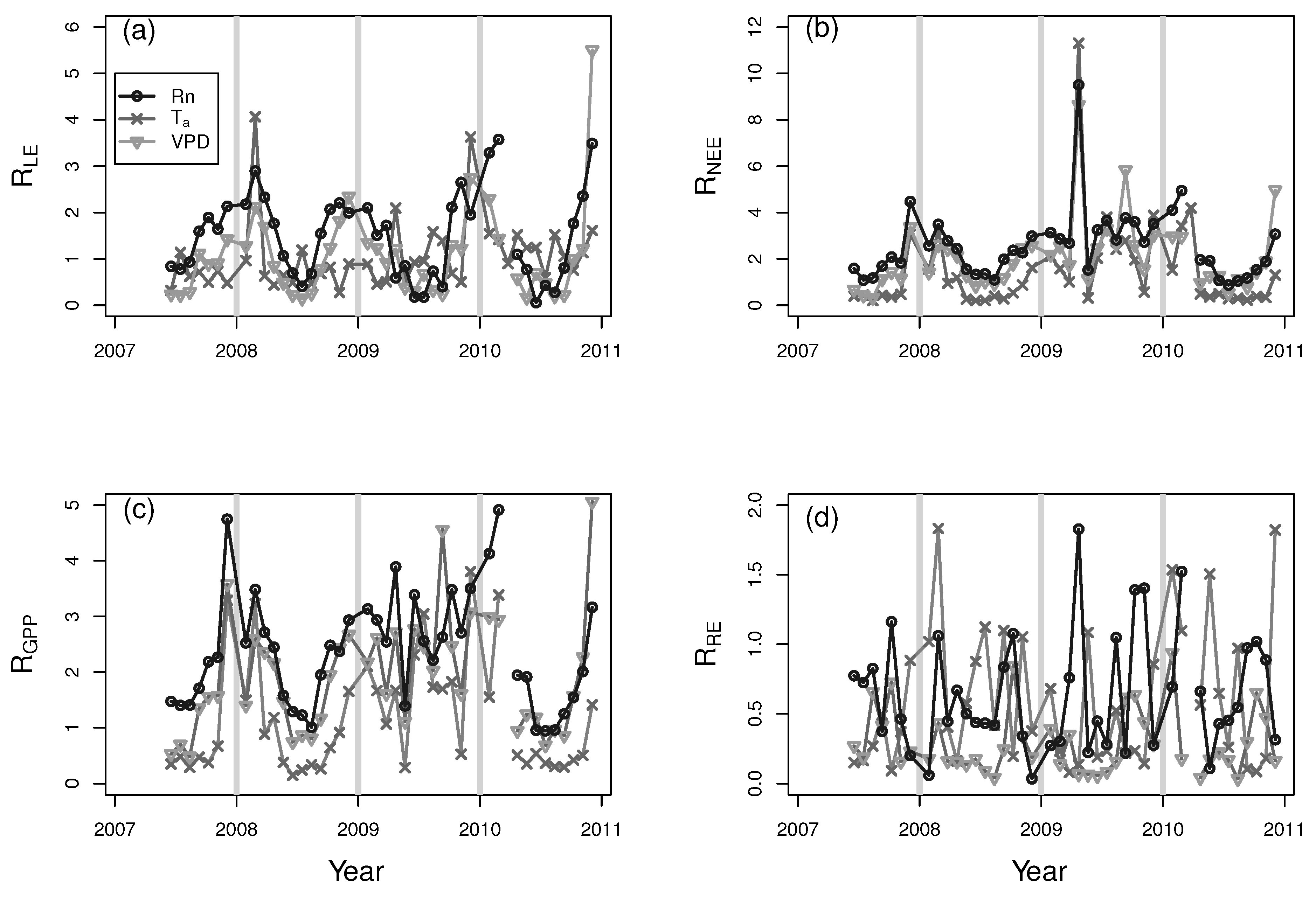
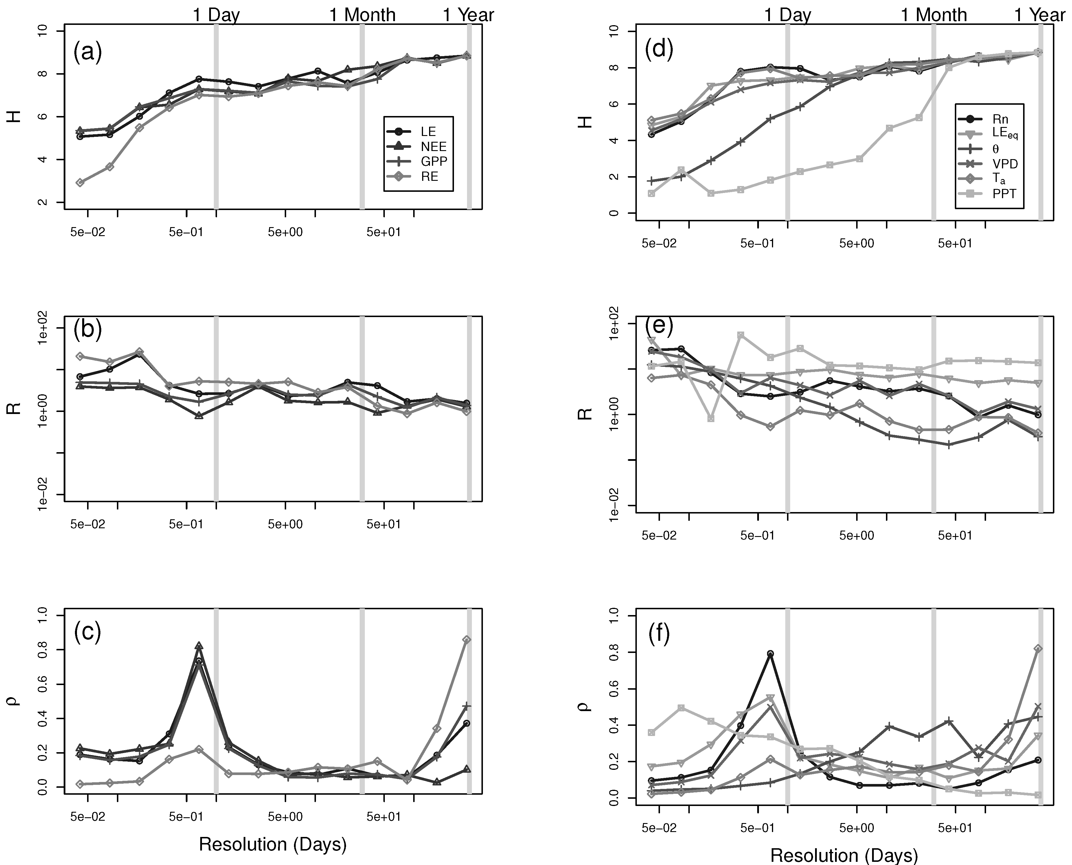
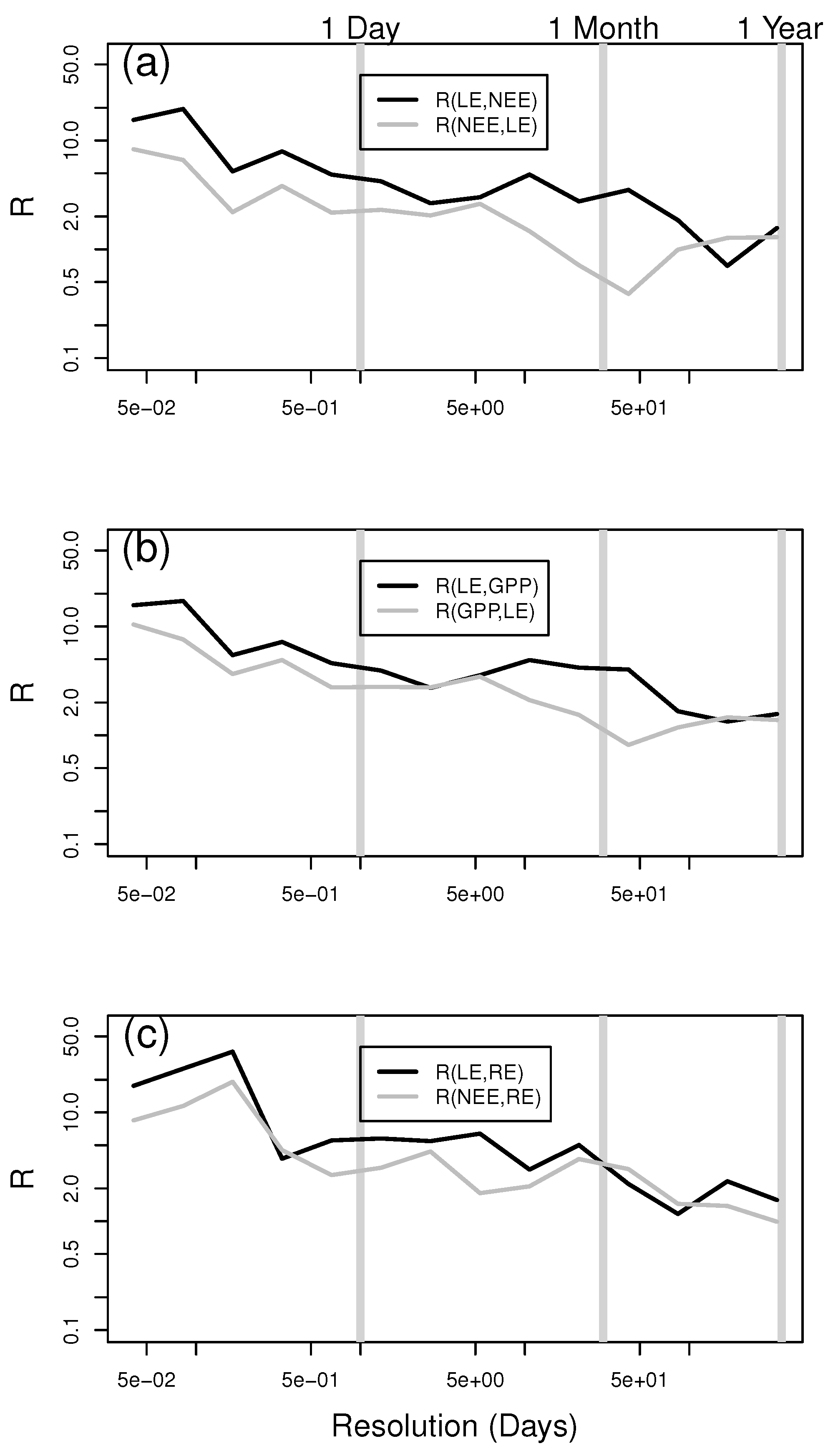
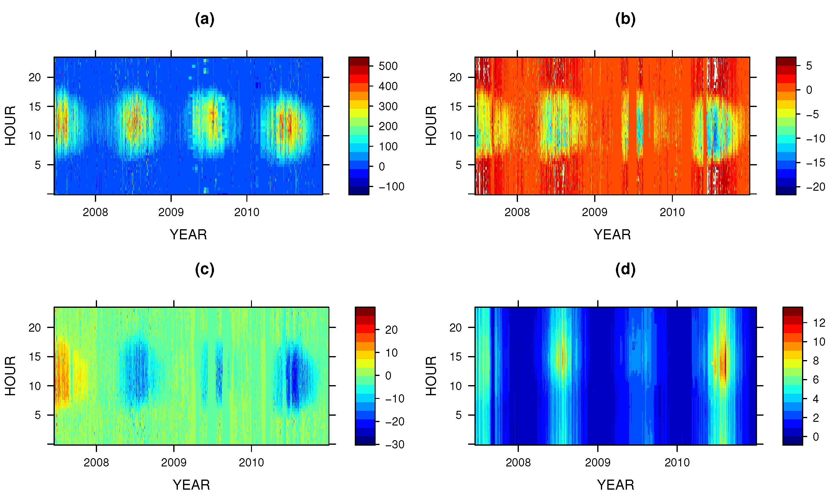
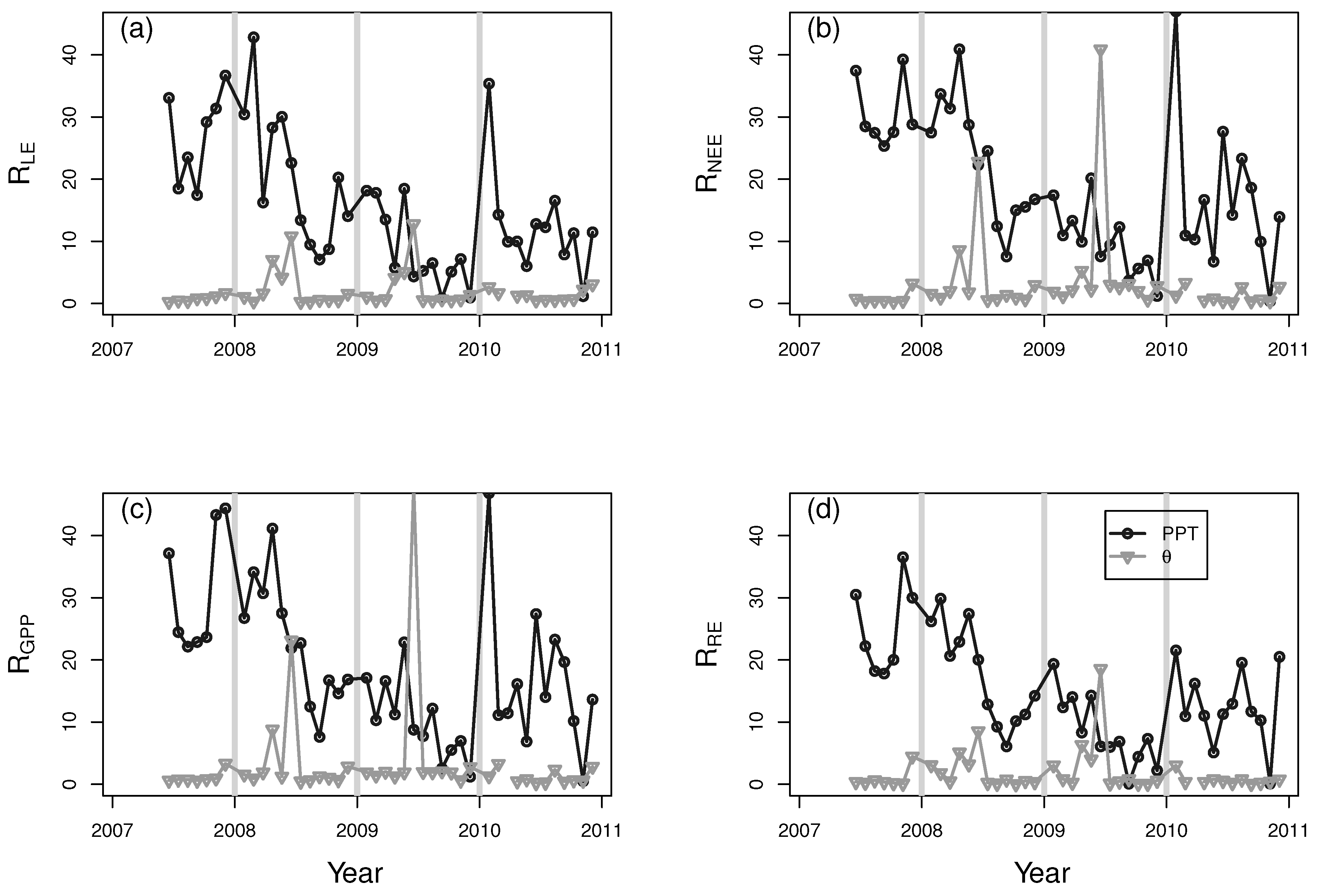
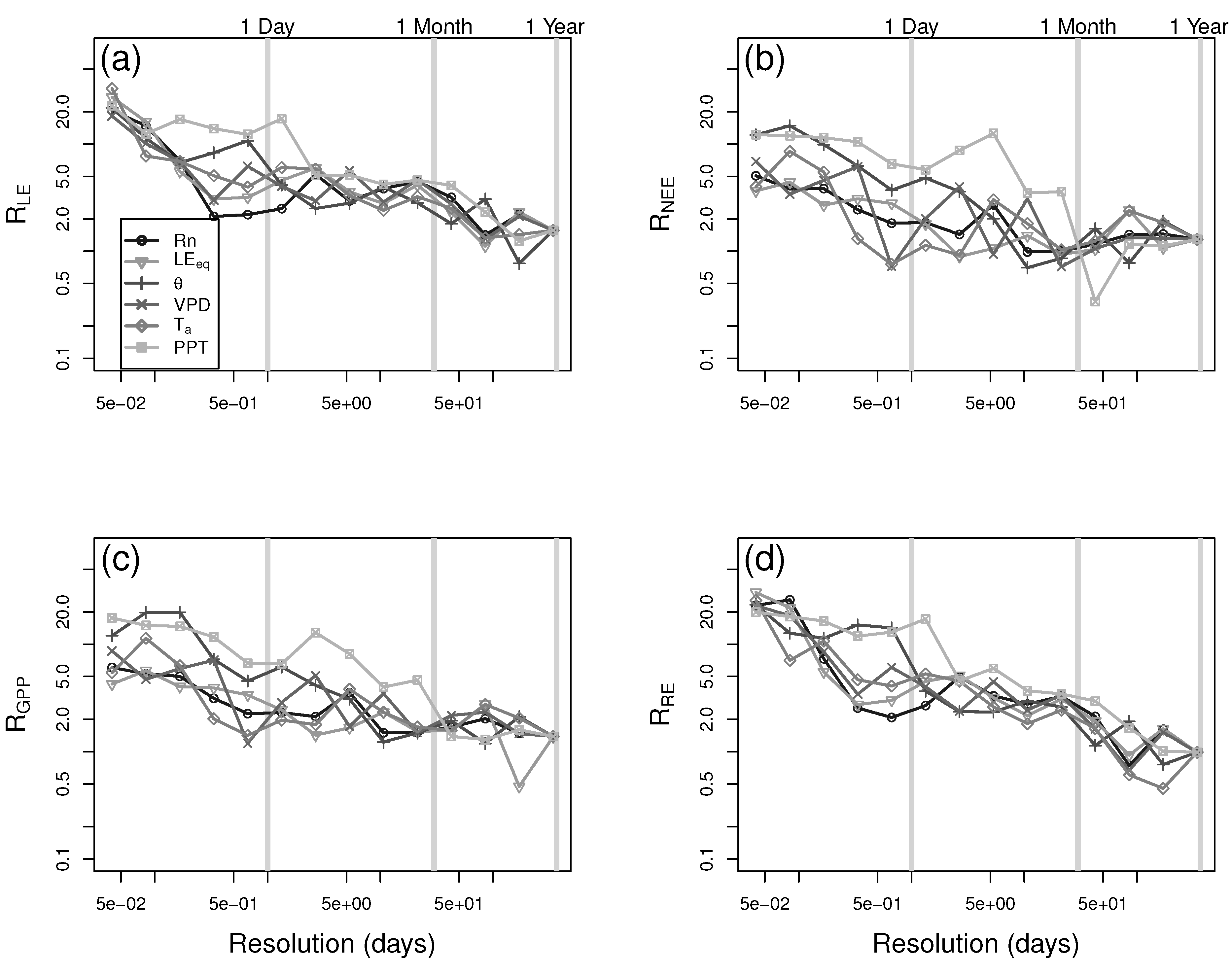
3. Results and Discussion

The time-series of gap-filled $LE$, $NEE$, $GPP$ and $RE$ are shown in Figure 1. We computed the monthly entropy values from the distribution of half-hourly flux measurements to assess their temporal variability (Figure 2a). Both fields generally show the same annual pattern, with the highest values of entropy in the summer and the lowest values in the winter. Summer values of $LE$ are fairly constant, with values of approximately $0.9$, while the winter values show a decreasing trend from 2008 ($0.8$) to the end of 2010 ($0.7$). The $NEE$ values in the summer are generally the same as the $LE$, with the exception of 2009, which contains a large proportion of gap-filled values. This decreases the overall entropy to minimum values of approximately ($0.6$), although it is highly variable.

Figure 1. Time-series of (a) latent heat; (b) net ecosystem exchange; (c) gross primary productivity; and (d) ecosystem respiration.

Figure 1. Time-series of (a) latent heat; (b) net ecosystem exchange; (c) gross primary productivity; and (d) ecosystem respiration.

Figure 2. Time-series of monthly entropy computed from half hour values of (a) latent heat and net ecosystem exchange; (b) gross primary productivity and ecosystem respiration; (c) net radiation, air temperature and vapor pressure deficit; and (d) precipitation and soil moisture.

Figure 2. Time-series of monthly entropy computed from half hour values of (a) latent heat and net ecosystem exchange; (b) gross primary productivity and ecosystem respiration; (c) net radiation, air temperature and vapor pressure deficit; and (d) precipitation and soil moisture.

The time-series of entropy for $GPP$ and $RE$ are shown in Figure 2b. The $GPP$ entropy follows the same trajectory as the $NEE$ values, ranging from approximately 0.6 to 0.9, while the $RE$ entropy is consistently higher (ranging between 0.85 and 0.95), with little discernible seasonal cycle.

Time-series of the entropy associated with the environmental variables of $Rn$, $T_a$ and $VPD$ are shown in panel (c) of Figure 2. The net radiation shows the same seasonal patterns as the $LE$ and $NEE$, with larger values in the summer and decreased values in the winter, although the overall range is reduced ($0.85$ to $0.95$). This dynamic is reduced for $VPD$, although it is still noticeable, while air temperature shows almost no seasonal variation in entropy. Time-series of $H\left(\theta \right)$ and $H\left(PPT\right)$ (panel (d) of Figure 2) are not characterized by a pronounced seasonal pattern. The precipitation entropy shows values of zero when these months had no precipitation.

The time-series of $H\left(LE\right)$, $H\left(NEE\right)$ and $H\left(GPP\right)$ all show a pronounced seasonal cycle, which most closely matches $H\left(Rn\right)$ (Figure 2c). Since the magnitude of the seasonal cycle in entropy decreases with the other variables, we interpret this as an indication of a decreased influence of the other variables to the observed fluxes. This is further investigated using the relative entropy.

The time-series of relative entropy between the environmental variables and the $LE$ is shown in panel (a) of Figure 3. The $R(LE,Rn)$ shows a pronounced annual cycle, reaching the highest values in the winter (approximately 3) and low values (0.5) in the summer. The seasonal cycles of the relative entropy of other environmental variables (notably for the $VPD$, though to a lesser extent than for $Rn$) and $LE$ follow similar patterns. Likewise, the $R(LE,T_a)$ shows a slight annual cycle, with peaks in the late winter or early spring.

Figure 3. Time-series of monthly relative entropy between the flux and the net radiation, air temperature and vapor pressure for (a) latent heat; (b) net ecosystem exchange; (c) gross primary productivity; and (d) ecosystem respiration.

Figure 3. Time-series of monthly relative entropy between the flux and the net radiation, air temperature and vapor pressure for (a) latent heat; (b) net ecosystem exchange; (c) gross primary productivity; and (d) ecosystem respiration.

The relative entropy between $NEE$ and environmental variables generally shows a strong annual cycle for all variables (Figure 3, panel (b)). The $Rn$ still shows the highest values in the winter, with values generally decreasing for the $VPD$ and $T_a$. The values in 2009 illustrate a change in the overall behavior, with values generally increasing from spring through the rest of the year.

Figure 3c shows the relative entropy between $GPP$ and the environmental variables. For the period of time up until 2009, there is a strong seasonal cycle for all variables peaking in the winter and decreasing in the summer. The $T_a$ maintains the lowest values, while the $R(GPP,Rn)$ is highest. All values are approximately constant through 2009 and decrease in 2010, possible returning to a peak in the winter of 2010–2011.

The $RE$ relative entropy values are shown in Figure 3d. All values are highly variable in the range of zero to 1.5 and show no clear annual cycle, such as that exhibited in Figure 3a, with lower R in the winter and higher in the summer. In the case of the $R(RE,VPD)$, it is slightly lower than the other environmental factors.

The relative entropy between the fluxes and θ and $PPT$ are shown in Figure 4. The same general behavior is seen for all the fluxes. Soil moisture shows low values throughout the year, with peaks in the spring of 2008 and 2009. These peaks are reduced for the $RE$ relative entropy, but of similar magnitude for the other fluxes. The relative entropy between the fluxes and $PPT$ is highly variable, showing little seasonal cycling, but possibly a longer term decreasing trend from mid-2007 until the beginning of 2010.

Figure 4. Time series of monthly relative entropy between the flux and the precipitation and soil moisture for (a) latent heat; (b) net ecosystem exchange; (c) gross primary productivity; and (d) ecosystem respiration.

Figure 4. Time series of monthly relative entropy between the flux and the precipitation and soil moisture for (a) latent heat; (b) net ecosystem exchange; (c) gross primary productivity; and (d) ecosystem respiration.

The seasonal variations in entropy and relative entropy are useful for showing the similarity of the distribution of different environmental variables and the distribution of half-hourly fluxes at the monthly time-scale. The seasonal cycle of the $LE$ relative entropies shows the lowest values during the summer seasons, implying a high similarity between the distribution of the $Rn$ and the $VPD$, in particular. It is well known that that these variables are driving variables of evaporative processes, and this is taken as support of the use of relative entropy as an indirect indicator of dynamics of the fluxes. We note that in winter, the radiation has higher relative entropies than the other variables. Although depending upon the winter, the $VPD$ and $T_a$ also have higher relative entropies. This would imply that the evaporative flux becomes dissimilar from the environmental variables, but it is also important to note the reduced magnitude of the flux during these periods.

The same temporal dynamics are observed with the relative entropies of the $NEE$. Although, in this case, it is the relative entropy with $Ta$ that has consistently lower values than either the radiation or vapor pressure deficit. This is supported by the well known respiration dependence upon temperature [37].

Next, we investigated how different temporal scales impact the water and carbon fluxes. The multiscale entropy for the fluxes are shown in Figure 5a. The wavelet decompositions are examined for periods of one hour up to one year, and we see that the general behavior in the entropy is to increase with time-scale. This increase is most pronounced in the sub-daily time-scales, with a slow increase in the daily to annual time-scales. This is seen for all fluxes, being more pronounced at the subdiurnal scale for $RE$.

Figure 5. (a) Multiscale entropy of the latent heat flux, net ecosystem exchange, gross primary productivity and ecosystem respiration; (b) the scalewise relative entropy for each flux in (a); (c) the multiscale correlation of each flux in (a); (d–f) are the same as (a–c) for net radiation, equilibrium evaporation, soil moisture, vapor pressure deficit, air temperature and precipitation. Note the log axes for the relative entropy plots.

Figure 5. (a) Multiscale entropy of the latent heat flux, net ecosystem exchange, gross primary productivity and ecosystem respiration; (b) the scalewise relative entropy for each flux in (a); (c) the multiscale correlation of each flux in (a); (d–f) are the same as (a–c) for net radiation, equilibrium evaporation, soil moisture, vapor pressure deficit, air temperature and precipitation. Note the log axes for the relative entropy plots.

The relative entropy between the decomposed fluxes and the observed flux was computed to examine the similarity of the distribution of the flux at various scales and the overall flux. Panel (b) of Figure 5 shows the multiscale relative entropy spectra (i.e., the relative entropy computed at each level of the wavelet decomposition) for the $LE$, $NEE$, $GPP$ and $RE$. The $LE$ and $RE$ relative entropy spectra show large peaks in the 0.25 day time-scales and otherwise a general reduction with increasing time-scale. There are slight peaks at the two-day and approximately one-month time-scales, as well. The $NEE$ and $GPP$ spectra also show a slight peak at two days and are otherwise approximately constant.

Figure 5c shows the correlation (ρ) between the wavelet decomposed and the original time-series. The correlations across scales are all fairly low (below ≈ 0.4), with the exception of the daily time-scale, which has the highest values for $NEE$, $LE$ and $GPP$. The $RE$ also exhibits a peak at the daily time-scale; however, it is of reduced magnitude (approximately 0.2) This indicates the overall dynamic of the $LE$, $NEE$ and $GPP$ fluxes are dominated by the daily variations. All of the fluxes also exhibit increased correlation with the annual scale.

The multiscale entropy for the environmental variables are shown in Figure 5d. The majority of the variables show similar values, with slightly different scales of the peak on the order of one day. The $Rn$ spectra peaks near the daily time-scale, while the peak is broader for air temperature (from the 0.5-day to the two-day scales). The $VPD$ shows a linear increase from the one hour scale. The θ spectra shows a greatly reduced variability at the shorter time-scales, approaching the other variables at time-scales on the order of five days. The precipitation spectra also shows reduced entropy until approximately the one-month time-scale. In addition to the other variables, we also computed the equilibrium evaporation, $L{E}_{eq}$, which rises to about the 0.25-day time-scale.

The relative entropy between the decomposed environmental variables and the observed variables is shown in Figure 5e. The multiscale relative entropy for all variables show the same general behavior, with peaks at the shortest time-scales. Precipitation is an exception, where the multiscale relative entropy shows a relatively flat spectra above the 0.5-day time-scale.

In addition, the scalewise correlation is shown in Figure 5f. The correlation is highest at the daily and annual time-scales for almost all variables. Only the soil moisture correlation shows a peak at approximately the monthly time-scale. At the daily time-scale, the overall correlation is highest for the radiation data ($Rn$ and $L{E}_{eq}$), then the $VPD$, with the $T_a$ being characterized by the smallest value. The soil moisture shows no peak at the daily time-scale. Again, $PPT$ shows different behavior, with an almost linear reduction in the ρ with the time-scale. This illustrates the dominance of the daily time-scale for these observations, with the exception of soil moisture and precipitation.

The next step in the analysis was to compute the relative entropy between different scales of the environmental variables and the flux data. The relative entropy between the variables and the latent heat flux is shown in Figure 6a. The highest values are seen in the shortest scales, with approximately log-linear decrease until the longest time-scale. At the subdiurnal time-scales, the $LE$ flux distribution is most similar (lowest R values) with the distribution of the radiation terms ($Rn$ and $L{E}_{eq}$), while precipitation and soil moisture have higher relative entropies. Above the five-day time-scale, the relative entropy values are all similar and exhibit a drop at approximately seasonal time-scales.

The $R(NEE,PPT)$ (Figure 6b) shows a higher value to slightly longer time-scales than the $R(LE,PPT)$, extending out to approximately two-days for the $LE$ and almost a month for the $NEE$. The relative entropy between the environmental variables and $NEE$ are more variable than for the $LE$, with the lowest values at the daily time-scale obtained for $T_a$ and $VPD$. The $PPT$ and θ are again the largest values, with the θ spectra approaching the other environmental fields at approximately the five-day scale. Unlike the $LE$ relative entropies, the $NEE$ shows more variability out to the monthly time-scale, beyond which the relative entropies are approximately constant. The $GPP$ relative entropy shows the same general behavior as the $NEE$ (Figure 6c).

Figure 6. Scalewise relative entropy (a) between latent heat flux and the environmental variables of net radiation, equilibrium evaporation, soil moisture, vapor pressure deficit, air temperature and precipitation; (b) between the net ecosystem exchange and the environmental variables; (c) between the gross primary productivity and the environmental variables; and (d) between the ecosystem respiration and the environmental variables.

Figure 6. Scalewise relative entropy (a) between latent heat flux and the environmental variables of net radiation, equilibrium evaporation, soil moisture, vapor pressure deficit, air temperature and precipitation; (b) between the net ecosystem exchange and the environmental variables; (c) between the gross primary productivity and the environmental variables; and (d) between the ecosystem respiration and the environmental variables.

The $RE$ relative entropy spectra shows the same range of values, but the daily time-scale is more closely linked to the radiation terms of $Rn$ and $L{E}_{eq}$ than $T_a$ and $VPD$, like the other components of the carbon cycle. In addition, the range of values observed across the variables is reduced beyond the five-day time-scale, implying that the variability of the $RE$ may be more closely linked to the same driving factors as the $LE$ flux (i.e., the radiation terms) than with the other carbon terms.

The multiscale relative entropy was used to ascertain which scales contribute the most information to the observed water and carbon fluxes (Figure 6). Both exhibit increases in the relative entropy at shorter time-scales, which indicates that the distribution of decomposed data are different from the distribution of the original time series. This is particularly true at subdiurnal time-scales. This corresponds to a decrease in the entropy at these time-scales (Figure 5), indicating that the distribution of these time-scales are less similar to the PDF observed fluxes. Thus, while more information is required, overall, they are less significant to the total flux. More importantly, we note that the environmental variables (lowest R values) vary between the $T_a$ and $VPD$ for ascertaining the $GPP$ and $NEE$ fluxes, while the radiation terms are most informative of the $LE$ and $RE$ fluxes.

The final analysis was to compute the relative entropy between the decomposed water and carbon fluxes to assess how much information is gained about the knowledge of one of the fluxes with respect to the other (Figure 7a). While both spectra generally decrease from the shortest time-scales, more information is necessary to characterize the distribution of $LE$, given the distribution of $NEE$, than to compute the distribution of $NEE$ from that of the $LE$, except at time-scales approaching 0.5 years, where the two values are approximately equal. We note that the $R(NEE,LE)$ is lowest at approximately monthly time-scales, implying that the $LE$ flux may be most directly used to assess the $NEE$ at this time-scale.

Figure 7. Scalewise relative entropy between (a) both the latent heat flux and net ecosystem exchange as a function of the wavelet decomposed versions of the other flux; (b) latent heat and gross primary productivity; and (c) latent heat and ecosystem respiration.

Figure 7. Scalewise relative entropy between (a) both the latent heat flux and net ecosystem exchange as a function of the wavelet decomposed versions of the other flux; (b) latent heat and gross primary productivity; and (c) latent heat and ecosystem respiration.

In addition, we computed the relative entropy between the $LE$ and $GPP$ and $RE$ fluxes (Figure 7 panels (b) and (c), respectively). $R(LE,GPP)$ shows the same general behavior as between the $LE$ and $NEE$. The relative entropy with respiration is slightly different at the monthly time-scale, with both values being equal.

4. Conclusions

We investigated the similarity of the distributions of water and carbon fluxes and some environmental variables using wavelets and information theory. From the relative entropies, we showed that the radiation terms contribute the most information about the distributions of $LE$ and $RE$. The distributions of $GPP$ and $NEE$ are more similar to $VPD$ and $T_a$. Soil moisture contributes information to the fluxes at approximately weekly time-scales, while the precipitation contributes information at monthly time-scales. These results highlight the utility of the relative entropy as a diagnostic measure of complex, non-linear interactions between environmental variables and water and carbon fluxes.

These results are consistent with findings using a variety of other techniques over a range of ecosystems [3,7,8]. We note here that the role of soil moisture and precipitation are reduced to variations at longer time-scales, which, while consistent with other studies, may not be a general finding for this site. This is due to the fact that for this study, we note that the observations were collected during higher than average precipitation in all years. This would imply that the role of soil moisture in limiting flux dynamics was reduced, as the system was rarely experiencing water limitation.

Information theory metrics are a relatively new technique for assessing biosphere-atmosphere interactions. Previous results [41,42,43] all show promise as quantitative measures of the transfer of information through the land-atmosphere system. This study is an additional example of the use of these techniques to examine the coupling between land surface fluxes and meteorological variables.

In particular, this study illustrates the utility of combining the information theory metrics with the wavelet decomposition to assess interactions across time-scales. We have used the wavelet-based information theory approach to allow for comparison of the role of different time-scales to the observed signal (multiscale entropy) or the impact of variability in environmental factors on the resultant flux (multiscale relative entropy). This type of analysis can be seen as an extension of prior work with wavelets, such as [39], in particular, the use of wavelets as an exploratory tool to identify the dominant scales of analysis. The present analysis could be applied across the Ameriflux or Fluxnet datasets in order to examine how the role of interactions at different temporal scales varies as a function of biome or environmental condition (e.g., drought vs. non-drought conditions). Another potential application of this technique is to assess the contribution of different time-scales in process-based models and to compare with the information spectra of the observations. Hence, it could serve to illustrate time-scales of poor model performance and, thus, provide a focus for model improvement.

The flow of information between the land surface and the atmosphere may be altered by the local impacts of global climate change. The coupling between the vegetation and the atmosphere interacts with the atmospheric boundary layer (ABL) via energy balance partitioning (the fraction of energy being used for sensible versus latent heat flux). The growth of the ABL will link water use by vegetation to the formation of clouds [44] and convective precipitation [45,46]. This leads to additional feedbacks between the precipitation, soil moisture and vegetation. This implies that the predicted changes in precipitation due to global climate change, which will potentially impact the central U.S. [47], may interact with local feedback mechanisms at the biosphere-atmosphere interface to further exacerbate the consequences of global change. A focus on the alterations to information flow due to these impacts may provide unique insights to examine these potential ramifications.

References

1. Mahecha, M.D.; Reichstein, M.; Jung, M.; Seneviratne, S.I.; Zaehle, S.; Beer, C.; Braakhekke, M.C.; Carvalhais, N.; Lange, H.; Le Maire, G.; Moors, E. Comparing observations and process-based simulations of biosphere-atmosphere exchanges on multiple time-scales. J. Geophys. Res. 2010. [Google Scholar] [CrossRef]
2. Katul, G.; Lai, C.T.; Schafer, K.; Vidakovic, B.; Albertson, J.; Ellsworth, D.; Oren, R. Multiscale analysis of vegetation surface fluxes: From seconds to years. Adv. Water Resour. 2001, 24, 1119–1132. [Google Scholar] [CrossRef]
3. Stoy, P.; Katul, G.; Siqueira, M.; Juang, J.; McCarthy, H.; Kim, H.; Oishi, A.; Oren, R. Variability in net ecosystem exchange from hourly to inter-annual time scales at adjacent pine and hardwood forests: A wavelet analysis. In Tree Physiology; Duke Univ, Nicholas Sch Environm & Earth Sci: Durham, NC 27708 USA, 2005; pp. 887–902. [Google Scholar]
4. Vargas, R.; Detto, M.; Baldocchi, D.; Allen, M. Multiscale analysis of temporal variability of soil CO2 production as influenced by weather and vegetation. Glob. Chang. Biol. 2010, 16, 1589–1605. [Google Scholar] [CrossRef]
5. Hong, J.; Kim, J. Impact of the Asian monsoon climate on ecosystem carbon and water exchanges: A wavelet analysis and its ecosystem modeling implications. Glob. Chang. Biol. 2010, 17, 1900–1916. [Google Scholar] [CrossRef]
6. Stoy, P.C.; Richardson, A.D.; Baldocchi, D.D.; Katul, G.G.; Stanovick, J.; Mahecha, M.D.; Reichstein, M.; Detto, M.P.; Law, B.E.; Wohlfahrt, G.; et al. Biosphere-atmosphere exchange of CO2 in relation to climate: A cross-biome analysis across multiple time scales. Biogeosciences 2009, 6, 2297–2312. [Google Scholar] [CrossRef]
7. Mahecha, M.D.; Reichstein, M.; Lange, H.; Carvalhais, N.; Bernhofer, C.; Grünwald, T.; Papale, D.; Seufert, G. Characterizing ecosystem-atmosphere interactions from short to interannual time scales. Biogeosciences 2007, 4, 743–758. [Google Scholar] [CrossRef]
8. Richardson, A.; Hollinger, D.; Aber, J.; Ollinger, S.; Braswell, B. Environmental variation is directly responsible for short- but not long-term variation in forest-atmosphere carbon exchange. Glob. Chang. Biol. 2007, 13, 788–803. [Google Scholar] [CrossRef]
9. Cowan, I. Fit, fitter, fittest: Where does optimisation fit in? Silva Fenn. 2002, 36, 745–754. [Google Scholar] [CrossRef]
10. Hopkins, A.; Del Prado, A. Implications of climate change for grassland in Europe: Impacts, adaptations and mitigation options: A review. Grass Forage Sci. 2007, 62, 118–126. [Google Scholar] [CrossRef]
11. Soussana, J.F.; Luscher, A. Temperate grasslands and global atmospheric change: A review. Grass Forage Sci. 2007, 62, 127–134. [Google Scholar] [CrossRef]
12. Scurlock, J.; Hall, D. The global carbon sink: A grassland perspective. Glob. Chang. Biol. 1998, 4, 229–233. [Google Scholar] [CrossRef]
13. Cleland, E.E.; Chiariello, N.R.; Loarie, S.R.; Mooney, H.A.; Field, C.B. Diverse responses of phenology to global changes in a grassland ecosystem. Proc. Natl. Acad. Sci. USA 2006, 103, 13740–13744. [Google Scholar] [CrossRef] [PubMed]
14. Li, S.G.; Eugster, W.; Asanuma, J.; Kotani, A.; Davaa, G.; Oyunbaatar, D.; Sugita, M. Response of gross ecosystem productivity, light use efficiency, and water use efficiency of Mongolian steppe to seasonal variations in soil moisture. J. Geophys. Res. 2008, 113. [Google Scholar] [CrossRef]
15. Chou, W.; Silver, W.; Jackson, R.; Thompson, A.; Allen-Diaz, B. The sensitivity of annual grassland carbon cycling to the quantity and timing of rainfall. Glob. Chang. Biol. 2008, 14, 1382–1394. [Google Scholar] [CrossRef]
16. Fay, P.A.; Kaufman, D.; Nippert, J.B.; Carlisle, J.D.; Harper, C.W. Changes in grassland ecosystem function due to extreme rainfall events: Implications for responses to climate change. Glob. Chang. Biol. 2008, 14, 1600–1608. [Google Scholar] [CrossRef]
17. Petrie, M.D.; Brunsell, N.A. The role of precipitation variability on the ecohydrology of grasslands. Ecohydrology 2012, 5, 337–345. [Google Scholar] [CrossRef]
18. Chen, X.; Rubin, Y.; Ma, S.; Baldocchi, D. Observations and stochastic modeling of soil moisture control on evapotranspiration in a Californian oak savanna. Water Resour. Res. 2008, 44, W08409. [Google Scholar] [CrossRef]
19. Polley, H.W.; Emmerich, W.; Bradford, J.A.; Sims, P.L.; Johnson, D.A.; Saliendra, N.Z.; Svejcar, T.; Angell, R.; Frank, A.B.; Phillips, R.L.; et al. Precipitation regulates the response of net ecosystem CO2 exchange to environmental variation on united states rangelands. Rangel. Ecol. Manag. 2010, 63, 176–186. [Google Scholar] [CrossRef]
20. Petrie, M.D.; Brunsell, N.A.; Nippert, J.B. Climate change alters growing season flux dynamics in mesic grasslands. Theor. Appl. Climatol. 2012, 107, 427–440. [Google Scholar] [CrossRef]
21. Hu, Z.; Yu, G.; Fu, Y.; Sun, X.; Li, Y.; Shi, P.; Wang, Y.; Zheng, Z. Effects of vegetation control on ecosystem water use efficiency within and among four grassland ecosystems in china. Glob. Chang. Biol. 2008, 14, 1609–1619. [Google Scholar] [CrossRef]
22. Makela, A.; Berninger, F.; Hari, P. Optimal control of gas exchange during drought: Theoretical analysis. Ann. Bot. 1996, 77, 461–467. [Google Scholar] [CrossRef]
23. Hari, P.; Makela, A.; Pohja, T. Surprising implications of the optimality hypothesis of stomatal regulation gain support in a field test. Aus. J. Plant Phys. 2000, 27, 77–80. [Google Scholar]
24. Reichstein, M.; Tenhunen, J.D.; Roupsard, O.; Ourcival, J.M.; Rambal, S.; Miglietta, F.; Peressotti, A.; Pecchiari, M.; Tirone, G.; Valentini, R. Severe drought effects on ecosystem CO2 and H2O fluxes at three Mediterranean evergreen sites: Revision of current hypotheses? Glob. Chang. Biol. 2002, 8, 999–1017. [Google Scholar] [CrossRef]
25. Van der Tol, C.; Meesters, A.G.C.A.; Dolman, A.J.; Waterloo, M.J. Optimum vegetation characteristics, assimilation, and transpiration during a dry season: 1. Model description. Water Resour. Res. 2008, 44. [Google Scholar] [CrossRef]
26. Cava, D.; Contini, D.; Donateo, A.; Martano, P. Analysis of short-term closure of the surface energy balance above short vegetation. Agric. For. Meteorol. 2008, 148, 82–93. [Google Scholar] [CrossRef]
27. Wever, L.; Flanagan, L.; Carlson, P. Seasonal and interannual variation in evapotranspiration, energy balance and surface conductance in a northern temperate grassland. Agric. For. Meteorol. 2002, 112, 31–49. [Google Scholar] [CrossRef]
28. Aires, L.; Pio, C.P.; Pereira, J.P. The effect of drought on energy and water vapour exchange above a mediterranean C3/C4 grassland in Southern Portugal. Agric. For. Meteorol. 2008, 148, 565–579. [Google Scholar] [CrossRef]
29. Aires, L.P.; Pio, C.P.; Pereira, J.S.P. Carbon dioxide exchange above a Mediterranean C3/C4 grassland during two climatologically contrasting years. Glob. Chang. Biol. 2008, 14, 539–555. [Google Scholar] [CrossRef]
30. Polley, H.; Dugas, W.; Mielnick, P.; Johnson, H. C3–C4 composition and prior carbon dioxide treatment regulate the response of grassland carbon and water fluxes to carbon dioxide. Funct. Ecol. 2007, 21, 11–18. [Google Scholar] [CrossRef]
31. Brunsell, N.A. Characterization of land-surface precipitation feedback regimes with remote sensing. Remote Sens. Environ. 2006, 100, 200–211. [Google Scholar] [CrossRef]
32. Jones, A.R.; Brunsell, N.A. Energy balance partitioning and net radiation controls on soil moisture–Precipitation feedbacks. Earth Interact. 2009, 13, 1–25. [Google Scholar] [CrossRef]
33. Brunsell, N.A.; Schymanski, S.J.; Kleidon, A. Quantifying the thermodynamic entropy budget of the land surface: Is this useful? Earth Syst. Dyn. 2011, 2, 87–103. [Google Scholar] [CrossRef]
34. Paw, U.K.; Baldocchi, D.; Meyers, T.; Wilson, K.B. Correction of eddy-covariance measurements incorporating both advective effects and density fluxes. Bound.-Layer Meteorol. 2000, 97, 487–511. [Google Scholar] [CrossRef]
35. Webb, E.; Pearman, G.; Leuning, R. Correction of flux for density effects due to heat and water vapour transfer. Q. J. R. Meteorol. Soc. 1980, 106, 85–100. [Google Scholar] [CrossRef]
36. Foken, T.; Wichura, B. Tools for quality assessment of surface-based flux measurements. Agric. For. Meteorol. 1996, 78, 83–105. [Google Scholar] [CrossRef]
37. Lloyd, J.; Taylor, J. On the temperature dependence of soil respiration. Funct. Ecol. 1994, 8, 315–323. [Google Scholar] [CrossRef]
38. Reichstein, M.; Falge, E.; Baldocchi, D.; Papale, D.; Aubinet, M.; Berbigier, P.; Bernhofer, C.; Buchmann, N.; Gilmanov, T.; Granier, A.; et al. On the separation of net ecosystem exchange into assimilation and ecosystem respiration: Review and improved algorithm. Glob. Chang. Biol. 2005, 11, 1424–1439. [Google Scholar] [CrossRef]
39. Kumar, P.; Foufoula-Georgiou, E. Wavelet analysis for Geophysical applications. Rev. Geophys. 1997, 35, 385–412. [Google Scholar] [CrossRef]
40. Kleeman, R. Measuring dynamical prediction utility using relative entropy. J. Atmos. Sci. 2002, 59, 2057–2072. [Google Scholar] [CrossRef]
41. Katul, G.; Lai, C.; Albertson, J.; Vidakovic, B.; Schäfer, K.; Hsieh, C.; Oren, R. Quantifying the complexity in mapping energy inputs and hydrologic state variables into land-surface fluxes. Geophys. Res. Lett. 2001, 28, 3305–3307. [Google Scholar] [CrossRef]
42. Ruddell, B.J.; Kumar, P. Ecohydrologic process networks: 1. Identification. Water Resour. Res. 2009, 45, 1–22. [Google Scholar] [CrossRef]
43. Ruddell, B.L.; Kumar, P. Ecohydrologic process networks: 2. Analysis and characterization. Water Resour. Res. 2009, 45, 1–14. [Google Scholar] [CrossRef]
44. Freedman, J.; Fitzjarrald, D.; Moore, K.; Sakai, R. Boundary layer clouds and vegetation-atmosphere feedbacks. J. Clim. 2001, 14, 180–197. [Google Scholar] [CrossRef]
45. De Ridder, K. Land surface processes and the potential for convective precipitation. J. Geophys. Res. 1997, 102, 30085–30090. [Google Scholar] [CrossRef]
46. Juang, J.-Y.; Katul, G.G.; Porporato, A.; Stoy, P.C.; Siqueira, M.S.; Detto, M.; Kim, H.-S.; Oren, R. Eco-hydrological controls on summertime convective rainfall triggers. Glob. Chang. Biol. 2007, 13, 887–896. [Google Scholar] [CrossRef]
47. Brunsell, N.A.; Jones, A.R.; Jackson, T.L.; Feddema, J.J. Seasonal trends in air temperature and precipitation in IPCC AR4 GCM output for Kansas, USA: Evaluation and implications. Int. J. Climatol. 2010, 30, 1178–1193. [Google Scholar] [CrossRef]