Towards Realising Secure and Efficient Image and Video Processing Applications on Quantum Computers

Abstract

Exploiting the promise of security and efficiency that quantum computing offers, the basic foundations leading to commercial applications for quantum image processing are proposed. Two mathematical frameworks and algorithms to accomplish the watermarking of quantum images, authentication of ownership of already watermarked images and recovery of their unmarked versions on quantum computers are proposed. Encoding the images as 2ⁿ-sized normalised Flexible Representation of Quantum Images (FRQI) states, with n-qubits and 1-qubit dedicated to capturing the respective information about the colour and position of every pixel in the image respectively, the proposed algorithms utilise the flexibility inherent to the FRQI representation, in order to confine the transformations on an image to any predetermined chromatic or spatial (or a combination of both) content of the image as dictated by the watermark embedding, authentication or recovery circuits. Furthermore, by adopting an apt generalisation of the criteria required to realise physical quantum computing hardware, three standalone components that make up the framework to prepare, manipulate and recover the various contents required to represent and produce movies on quantum computers are also proposed. Each of the algorithms and the mathematical foundations for their execution were simulated using classical (i.e., conventional or non-quantum) computing resources, and their results were analysed alongside other longstanding classical computing equivalents. The work presented here, combined together with the extensions suggested, provide the basic foundations towards effectuating secure and efficient classical-like image and video processing applications on the quantum-computing framework.

1. Introduction

Computer science and computer engineering are disciplines that have transformed every aspect of human endeavour. In these fields, exciting and cutting-edge research about new models of computation, new materials and techniques for building computing hardware have been broached with many of them already realised [1]. Novel methods for speeding-up certain tasks, and building bridges between computer science and several other scientific fields that allow scientists to both think of natural phenomena as computational procedures as well as in simulating natural processes have also been proposed [2,3].

Quantum computation is one such interdisciplinary field that offers a new perspective in terms of high performance computing, with algorithms that solve problems considered intractable for today's computing technologies [4]. With its physical realisation is the promise of improved miniaturisation, massive performance speed-up for certain tasks [4,5], new levels of protection in secure communication [4]; information processing; and ultra-precise measurements [5]. These theoretical discoveries and promising conjectures have positioned quantum computation as a key element in modern science [3].

Physical implementations of the qubit, the information carrier on the quantum-mechanical framework, and operations to manipulate it are available from many approaches. Among these are implementations based on nuclear magnetic resonance; ion, atom and cavity electrodynamics; solid state, and superconducting systems [6]. Other technologies being considered for realising physical quantum hardware include those based on quantum dot and optical or photonic systems [4,6].

Indeed, one of the major problems now facing the field of quantum information is the relative dearth of applications; to the point where many scientifically-minded outsiders to the field believe that the only application of quantum computing is “factoring” [7].

However, a growing number of quantum computing algorithms with potential or (in some cases) proven applications in several branches of science and technology have been suggested. One such area to have emerged into the spotlight is the new field of quantum image processing (QIP), which seeks to extend traditional image processing and its applications to (or using) quantum computing [1].

On quantum computers, however, research on image processing is still in its infancy. As a result, the field is still bedeviled with so many questions. To start with, what makes an image or how is the best way to represent images on quantum computers? Secondly, what should be done to prepare and process the quantum images? Then, for us to really say the field has matured we should be capable of performing some basic image processing tasks leading to the realisation of some high-level applications using quantum-computing hardware, following which we need to gradually advance these capabilities to allow for the accomplishment of more advanced and robust image processing applications and tasks.

Research in the field began with proposals to represent quantum images such as: Qubit Lattice, wherein the images are two dimensional arrays of qubits in [8,9]; in Real Ket [10], the images are quantum states having grey-levels as coefficients of the states; and in the Flexible Representation for Quantum Images (FRQI) [1,11,12], the images are normalised states that capture the essential information about every point in an image such as its colour and their corresponding positions.

Quantum based transformations with likely applications in image processing such as the quantum Fourier transform [13], quantum discrete cosine transform [1,13,14,15], quantum wavelet transform [16] have also been proposed.

Manipulating some of these transformations, the realisation of some high-level image processing tasks on quantum computers has been explored [17,18,19,20,21,22,23,24].

In terms of applications, available literature on quantum image processing can be broadly classified into one of two groups. In the first, which we shall refer to as quantum-inspired image processing [1,20], the aim is to exploit some of the properties responsible for the potency of quantum computing algorithms in order to improve some well-known classical or digital (i.e. conventional or non-quantum) image processing tasks and applications. Some of the available literature that fall under this group include: the work by Beach et al. [25], which concentrated on showing that existing quantum computing algorithms (such as Grover's algorithm [26]) are applicable to image processing tasks. In a different application [27], the use of quantum computing and reverse emergence in classical image processing was discussed. The key idea involved in this work is the use of cellular automata as a complex system and quantum inspired algorithms as a search strategy. Specifically, the main concern of the work was on how to cope with the complexity of the emergent properties and structures arising from the use of cellular automata by using quantum evolutionary algorithms for training cellular automata to perform image processing tasks.

As interest in the quantum computing field continues, culminating in the realisation of physical quantum computing hardware, it is envisaged that using any (or all) of the representations alluded to earlier, quantum images will be made physically available. The second group of the available literature in QIP derives its inspiration from this expectation and, hence, such research focuses on extending classical image processing tasks and applications to the quantum computing framework. Accordingly, such work will be referred to as classically-inspired quantum image processing [1,20].

In terms of technologies to physically realise quantum image processing hardware, the general problem of the quantum noise in multi-pixel measurement of an optical image characterised by the intrinsic single-mode and multi-modes of light was considered in [28]. Then, using transverse mode decomposition for each type of possible linear combination of the pixel's output an exact expression of the detection mode was obtained. They also considered ways to reduce noise in one or several simultaneous measurements. In another work [14], the bound to the maximum achievable sensitivity in the estimation of a scalar parameter from information contained in an optical image in the presence of quantum noise were discussed. Their work confirmed that this limit is valid for any image processing protocol and is calculated in the case of non-classical illumination.

More recently, [21] gathered the strewed optical and photonic quantum computing technologies to present an interesting insight into how FRQI QIP can be accomplished using these technologies and/or their modifications.

In the meantime, the goal of QIP in general and FRQI-based QIP in particular is to exploit the properties of quantum mechanics in order to realise state-of-the-art image processing algorithms capable of rivalling their classical counterparts [1].

Based on the foregoing discussions, it is, therefore, apparent that this review itself adds to the classically-inspired quantum image processing literature and its main contribution is tailored towards extending some auspicious classical image processing applications to the quantum-computing domain.

For example, experience with classical images suggests that, when realised, quantum images will be susceptible to all kinds of abuse and disputes regarding their ownership [1,18], hence, making it imperative that we consider algorithms best suited for safeguarding the proprietorship of the images.

Building good quantum algorithms, which are essential for executing any quantum information processing, is a difficult task especially because quantum mechanics is a counter-intuitive theory and intuition plays a major role in algorithm design. A quantum algorithm is considered good not only because it can perform its intended task but it must also do it better, i.e. be more efficient than already existing (usually, classical) ones.

In the quantum circuit models of computation, designing efficient circuits is necessary to realise and analyse any quantum algorithm. The main resources that make up these circuits consist of a succession of basic unitary gates that act on one or two qubits only. Many elementary gates including single qubit gates, Pauli gates, controlled-NOT or CNOT and Toffoli gates for quantum computation were introduced in [6,29].

In the course of our review herein, we shall assume a general understanding of these basic rudiments of quantum mechanics and quantum computation. Hence, we shall proceed with a very succinct discussion, in the next section, on the approaches used to execute a computation in the quantum sense.

The remainder of the review is outlined as follows. In Section 3, we review the FRQI representation including its preparation to obtain the initialised and FRQI image state. Exploiting the flexibility in the manner in which the FRQI representation captures the information about colours and corresponding positions of every point in an image, two sets of transformation operations targeting the chromatic and spatial (geometric) contents of the image, the CTQI and GTQI respectively, were proposed in [30,31,32] and will also be reviewed in the same section (i.e. Section 3).

We complete the section with a discussion on the restricted variants of these transformations to realise the rGTQI and rCTQI transformations that allow the confinement of any predetermined transformation on the spatial or chromatic content of smaller sub-areas of the image. These restricted geometric transformations with their low complexity provide the foundation on which our proposed scheme to watermark and authenticate ownership of already watermarked quantum images, WaQI [1,17,18], is built. The review on WaQI is the main subject of Section 4. In it, the classical content of each input image and watermark signal as a pair, is blended together to produce a bespoke map that dictates the composition of the quantum watermark embedding and authentication circuits for each image-watermark pair. By targeting the geometric content of the cover image, the WaQI guarantees a robust, blind, keyless, and efficient scheme.

Later in Section 5, our attention shifts to the intricacies between the imaging system and the likely technologies for its future implementation, such as photonic or optical quantum technologies, using which a revised reformulation of the FRQI representation is proposed in order to realise greyscale versions of the FRQI quantum images. Using this modified encoding of the image, a bi-level scheme, which we also refer to as the greyscale version of WaQI or simply WaGQI [1,20]; to watermark the cover images and recover their unmarked (pristine) versions is implemented. The first tier of the proposed scheme involves embedding a conspicuous watermark logo in a predetermined sub-area of the cover (host or original) image, whilst in the second tier the same watermark signal is embedded so that its content traverses the remainder of the image in an obscure or invisible manner. The main resources to accomplish the WaGQI scheme are restricted variants of the CTQI transformations.

By generalising DiVincenzo's five criteria [33] for realising physical quantum-computing hardware, our proposed framework to represent and produce quantum movies is reviewed in Section 6. The three devices realised from this generalisation namely: the Quantum CD, Quantum Player and Movie Reader, each of which performs certain tasks as would be required to efficiently represent and produce movies on quantum computers [19] are also reviewed. Concatenated, these components together facilitate the proposed framework for quantum movie representation and production as reviewed in this section.

Section 7 presents insights into future perspectives related to how the proposed protocols can be improved and likely directions for their physical realisation.

The algorithmic frameworks presented in this work provide the basic foundation for accomplishing classical-like image and video processing applications and tasks on quantum computing hardware. This would hopefully motivate the interest of practitioners and researchers in the field of quantum computation and quantum information to pursue physical realisation of application-specific quantum hardware, thereby accelerating the quest to realise commercially viable quantum computing hardware.

2. The Quantum Computational Models

An algorithm is a procedure to perform a certain task on a computer. Although independent of the computational model, it is usually beneficial to design an algorithm with a particular model in mind because in doing so the resources needed for its execution that are more advantageous than other models would be taken into consideration [1].

Computation, in the quantum sense, comprises of a sequence of unitary transformations affecting simultaneously each element of the superposition, generating a massive parallel data processing albeit within one piece of hardware [1,20]. The efficiency of an algorithm is then derived in terms of the number of such unitary transformations. The smallest unit to facilitate such computation, the qubit, has logical properties that are inherently different from its classical counterpart, the bit. While bits and their manipulation can be described using two constants (0 and 1 or true and false) and the tools of Boolean algebra, qubits, on the other hand must be discussed in terms of vectors, matrices, and other tools of linear algebra. Exploiting the quantum mechanical properties of the quantum computing paradigm, such as the optimisation of resources like qubits, entanglement, elementary operations and measurements as necessary for an efficient experimental implementation of an algorithm, a number of models have been suggested to execute a computation.

For our review of the quantum computational models that follows, we will rely, in part, on the elegant and thorough work presented in [34] and [35] and other references therefrom.

The first of these models is the circuit model of computation, wherein, computation is run by a sequence of unitary gates and represented by its circuit diagram, with the connecting wires representing the (logical) qubits that carry the information, and the information is processed by the sequence of quantum gates akin to the manner logic gates can be combined to achieve a classical computation. This computational model gained further accedence when it was proved that any quantum circuit can be constructed using nothing more than quantum gates on one qubit and the controlled-NOT (CNOT) gates on two qubits. This limited but sufficient set of gates is named a universal set of gates [6,29,36]. In the end, the result of the computation is read out by performing projective measurements on the qubits. The problem of designing quantum algorithms is largely the task of designing the corresponding quantum circuits. This computational model is also referred to as unitary-evolution-based quantum computation model, but we shall just refer to it as the UQC computational model.

The measurement-based quantum computation (MQC) is an alternative strategy that relies on effects of measurements on an entangled multi-partite resource state to perform the required computation [34,37]. This novel strategy to overcome the perceived shortcomings of the circuit model of quantum computation has been realised experimentally using single-qubit measurements which are considered “cheap” [1,19,36]. By contrast, computation in the MQC is run by a sequence of single-qubit adaptive projective measurements on the graph state [34]. All measurement-based models share the common feature that measurements are not performed solely on the qubits storing the data. The reason is that doing so would destroy the coherence essential to quantum computation. Instead, a variant of the MQC specifies that ancillary qubits be prepared, and then measurements are used to ensure interaction between the data with the ancilla. By choosing appropriate measurements and initial states of the ancilla carefully, we can ensure that the coherence is preserved. Even more remarkable is the fact that with suitable choices of ancilla and measurements, it is possible to realise a universal set of quantum gates. Often, this variant of the MQC is called the ancilla-driven quantum computation (ADQC) [1,19,38].

In the ADQC, the ancilla A is prepared and then entangled to a register qubit using a fixed entanglement operator E [19]. A universal interaction between the ancilla and register is accomplished using the controlled-Z (CZ) gate and a swap (S) gate, and then measured. An ADQC with such an interaction allows the implementation of any computation or universal state preparation. This is then followed by single qubit corrections on both the ancilla and register qubits. The ADQC is also considered as a hybrid scheme of the circuit model, since computation involves a sequence of single and two-qubit gates implemented on a register. Similar to all the measurement-based models, the standard ADQC uses a fully controlled ancilla qubit, which is coupled sequentially to one or at most two qubits of a register via a fixed entanglement operator E. After each coupling, the ancilla is measured in a suitable basis, providing a back action onto the register. This implements both single- and two-qubit operations on the register qubits.

Both the UQC and the MQC (and its variants) are universal, can simulate each other and possess their own advantages. On one hand, no preparation of a resource state and classical information processing is required in the UQC [34]. On the other hand, measurements in the MQC are simpler to execute than unitary gates to perform the computation. In practice, the difficult part in UQC is to implement multi-qubit gates, while for the MQC it is to prepare a universal graph state. The bigger the graph state, the more difficult it is to control and protect it from noise. Based on these observations, and to fulfill the need for experimental optimisation, the hybrid quantum computation model (HQC) was introduced [34].

The HQC employs the MQC only to implement certain multi-qubit gates, which are complicated in the UQC. These multi-qubit gates are realised by preparing small (non-universal) graph states in one go followed by single shot of measurements in the HQC. The implementation of an arbitrary single qubit operation is rather straightforward in the UQC, but it requires a chain of five qubits graph state in the MQC. Therefore, the HQC chooses unitary evolution from the UQC to execute single-qubit gates. Furthermore, the two-qubit controlled-Z (CZ) operations themselves are part of the experimental setup for constructing the graph states, and for this, we have to execute the computation via unitary evolutions.

Like other models of computation, the UQC, which forms the core of the algorithmic frameworks discussed in this review are based on, has five requirements widely recognised as the criteria for realising any physical quantum system [20,34]. The first of these requirements is quantum state preparation, the result of which is a scalable physical state with well-characterised qubits. In addition, this state can be initialised in a way that isolates it from the environment. Often, a quantum state can be obtained (prepared) from its classical equivalent [18]. A quantum state can only be manipulated using a universal set of quantum gates (or appropriate measurements in the case of MQC). In such gates, time flows from left to right with horizontal lines, called quantum wires representing separate qubits that comprise the quantum register [20,34]. One-qubit operations and gates are represented by single qubit wires and two-qubits by using perpendicular lines to show interaction, and so entanglement, between relevant qubits.

Figure 1. The three stages of the circuit model of quantum. The figure was adapted from [35] from where additional explanation can be obtained.

Figure 1. The three stages of the circuit model of quantum. The figure was adapted from [35] from where additional explanation can be obtained.

Figure 1 depicts the universal circuit model of computation. In the first step, the qubits are initialised in a standard state such as $|000\hspace{0.17em}\cdots \hspace{0.17em}0\rangle$. The algorithm, represented by a big unitary operation, U, over all the qubits, is executed through a set of single and two qubit gates from a universal gate set. Arbitrary single qubit operations and the two-qubit CNOT gate have been chosen here. The final stage is the readout of the qubits to recover the classical information needed [6,35].

In modelling a quantum circuit, complex transformations are broken into simpler gates, i.e. single qubit gates such as the NOT, Hadamard, or Pauli gates and controlled two-qubit gates like the controlled NOT gates [19,29,39,40,41]. Recently, the following set of gates have found wide acceptance in the literature as the elementary or basic quantum gates largely arising from the universality of the set and the ease with which very complex circuits can decomposed in terms of them.

NOT gate (N). This is a single qubit gate, which inverts the content of the qubit it operates upon.

• Controlled-NOT or CNOT gate (C). It is a two-qubit gate and the content of the target qubit is inverted if and only if the control qubit is 1.
• Toffoli gate (T). This is a controlled-CNOT gate, thus, making it a three-qubit gate comprising two controls and a single target qubit. The target qubit is inverted if and only if both control qubits are 1s.

Together these gates are often referred to as the NCT gate [19,29,39,40,41].

Finally, qubit-specific measurements are employed in order to obtain the classical read-out of the new, i.e. the transformed or manipulated state, leading to a collapse (loss) of the hitherto quantum state [6,19].

In the next section, we review the model-independent representations for images on quantum computers with focus on the FRQI quantum image representation as the cornerstone of the algorithmic frameworks to be presented in latter sections of the review.

3. Quantum Image Processing

The pioneering role of research that gave birth to what is today referred to as quantum image processing (QIP) can be attributed to the work by Venegas-Andraca et al. [2,9,37] and that by Lattore [10]. They independently proposed the qubit lattice and Real Ket representations for a quantum image, respectively. The qubit lattice [2,9] is based on the idea that the frequency of the physical nature of colour could represent a colour instead of the RGB and HIS models, so a colour could be represented by only a 1-qubit state and an image could be stored in a quantum array [37,42]. Meanwhile, in Real Ket [10] the image is a quantum state having grey levels of coefficients of the state.

These innovative representations to encode images on the quantum computing framework set the stage for Le et al. to propose the flexible representation for quantum images (FRQI) [1,11,12]. In this representation, the images are normalised states that capture the essential information about every point in an image such as its colour and their corresponding positions.

More recently Zhang et al. [43] suggested the novel enhanced quantum representation (NEQR) for images, which they claim improves the FRQI representation. Instead of using the probability amplitude of the qubit to encode information about the image, as in the FRQI representation, their proposed NEQR uses the basis states of a qubit sequence to store the greyscale value of each pixel in an image for the first time.

The number of applications that are based on the original FRQI representation is, however, enough evidence to suggest its widespread acceptance. Exploiting its adroitness, two operations to manipulate the chromatic and spatial contents of an image, the CTQI [1,32] and GTQI [1,30,31] operations, were proposed. Some of the algorithms that utilise the FRQI representation and its transformations include those to watermark, authenticate ownership of and recover watermarked quantum images [1,17,18,20,44,45]; represent and produce movies on quantum computers [1,18]; undertake image database search [23,24]; image encryption [46] and image compression [42]. More recently, there have been attempts to remodel the FRQI representation to capture greyscale quantum images [20]; encode multi-channel (RGB) versions of the images [22]; and for more efficient image storage and retrieval [42].

The prospects of extending some already established quantum-based transformations, few of which have been proven to be more efficient than their classical versions [1,12], that have direct impacts on image processing such as the Fourier transform [5,36], discrete cosine transform [6,13], wavelet transform [16] make QIP more appealing.

The formulation of the quantum Fourier transform whose classical analogy is employed as the basis of classical convolution and correlation operations further raised a lot of hope for the prospect of realising applications that could utilise these operations such as image processing, signal processing, pattern matching and many more on the quantum computing framework. However, these hopes have been dashed with violation of some key laws of quantum mechanics by the component step-wise multiplication of vectors after the initial Fourier transforms, which is a key step of the convolution and correlation operations, thereby, foreclosing the possibility of directly performing the convolution and correlation operations on a quantum state [20,25]. The no-cloning theorem [47] provides another lack of accessibility suffered by quantum information in comparison to its classical counterpart [18]. This theorem provides a rather peculiar commentary on the impossibility of directly copying the information encoded in a quantum state. Together, these provide some impossible processing operations on quantum computers, hence, further demonstrating the fundamental difference between quantum and classical information processing.

This review is essentially dedicated to reviewing some of the algorithmic frameworks that have made FRQI-based QIP an interesting academic pursuit. Therefore, we will start, in the sequel, by reviewing the FRQI representation for quantum images including its preparation and transformation to accomplish the state-of-the-art image processing applications presented in latter parts of the review.

3.1. Flexible Representation for Quantum Images, FRQI

In digital image processing, an image is a sampled and mapped grid of dots or picture elements (pixels) capturing a snapshot taken of a scene or scanned from documents, such as photographs, manuscripts, printed texts, and artwork [1]. Each pixel is assigned a tonal value (black, white, shades of grey or colour), which is represented in binary code (zeros and ones). The binary digits ("bits") for each pixel are stored in a sequence by a computer and often reduced to a mathematical representation (compressed). The bits are then interpreted and read by the computer to produce and display (or print) a version that can be understood by humans [1].

Inspired by the aforementioned interpretation of an image and also by the human perception of vision in general, a quantum analogue to capture, store and manipulate information about the colours and the corresponding positions of every point in images on quantum computers, named the flexible representation for quantum images, or simply FRQI representation was first proposed in [11] and later reviewed in [1,12] and [20,22,48]. It is so named to account for its flexibility both in usage and transformations on it that facilitates the realisation of more complex image processing applications. This proposal integrates information about an image into a quantum state having its formula in Equation (1):

$$|I\left(\theta \right)\rangle =\frac{1}{2^n}{\displaystyle \sum _{i=0}^{2^{2n}-1}|c_i\rangle \otimes |i\rangle ,}$$

(1)

where:

$$|c_i\left(\theta \right)\rangle =\cos {\theta }_i|0\rangle +\sin {\theta }_i|1\rangle$$

(2)

and:

$${\theta }_i\in \left[0,\frac{\pi }{2}\right],i=0,\hspace{0.17em}1,\dots ,2^{2n}-1$$

(3)

$|0\rangle$ and $|1\rangle$ are the 2²ⁿ-D computational basis quantum states, $|i\rangle ,\hspace{0.17em}\hspace{0.17em}\hspace{0.17em}i=0,1\dots ,2^{2n}-1$ are 2²ⁿ-D computational basis quantum states, and $\theta =({\theta }_0,{\theta }_1,\mathrm{...}{\theta }_{2^{2n}-1})$ is the vector of angles encoding the colours in the image. There are two parts in the FRQI representation of an image: $c_i\left(\theta \right)$ and $|i\rangle$, which encode information about the colour and corresponding positions of all the points in the image respectively.

For 2-D images, the spatial information $|i\rangle$ is the grid information about the location of every point encoded by the position qubits that comprises of two parts: the vertical and horizontal co-ordinates. In 2n-qubit systems for preparing quantum images, or n-sized images, the vector $|i\rangle$ is defined as:

$$|i\rangle =|y\rangle |x\rangle =|y_{n-1}{y}_{n-2}\dots y_0\rangle |x_{n-1}{x}_{n-2}\dots x_0\rangle , \text{for} x_i,y_i\in \left\{0,1\right\}$$

(4)

where the first n-qubits $y_{n-1}{y}_{n-2}\dots y_0$ encode information along the vertical coordinate and the second n-qubits $x_{n-1}{x}_{n-2}\dots x_0$ encode information about the horizontal coordinates. The FRQI state is a normalised state given by:

$$\Vert |I\left(\theta \right)\rangle \Vert =\hspace{0.17em}\frac{1}{2^n}\hspace{0.17em}\sqrt{{\displaystyle \sum _{i=0}^{2^{2n}-1}\left({\cos }^2{\theta }_i+{\sin }^2{\theta }_i\right)}}=1$$

(5)

An example of a 2 × 2 FRQI quantum image with its corresponding state is presented in Figure 2.

Figure 2. A simple FRQI image and its quantum state.

Figure 2. A simple FRQI image and its quantum state.

To effectively capture all the information about the colour and position of a $2^n\times 2^n$-sized FRQI image, a total of 2n+1 qubits are required [1] as shown in the generalised circuit of the FRQI representation in Figure 3.

Figure 3. Generalised circuit showing how information in an FRQI quantum image state is encoded.

Figure 3. Generalised circuit showing how information in an FRQI quantum image state is encoded.

A unitary transformation, P=RH, is required to achieve the preparation process of an FRQI quantum image based on the polynomial preparation theorem (PPT) [1,11,12]. The transforms R and H that are used to prepare the FRQI quantum image are the Hadamard and controlled-rotation transformations respectively. Given a vector $\theta =({\theta }_0,{\theta }_1,\mathrm{...}{\theta }_{2^{2n}-1})$ of angles satisfying Equation (3), the unitary transform P turns the quantum computer from the initialised (vacuum) state, ${|0\rangle }^{\otimes 2n+1}$ to the FRQI state, $|I\left(\theta \right)\rangle$. The PPT theorem that is used to accomplish this specifies that a number that is quadratic to the total $2^{2n}$ angle values ${\theta }_i,\hspace{0.17em}i=0,1,\cdots ,2^{2n}-1$, or more precisely $2^{4n}-3\cdot 2^{2n}+2n$ simple operations, are required to prepare an n-qubit FRQI quantum image.

Figure 4 illustrates the transformations required to execute the P transformation based on the PPT theorem.

Figure 4. Illustration of the two steps of the PPT theorem to prepare an FRQI image.

Figure 4. Illustration of the two steps of the PPT theorem to prepare an FRQI image.

The polynomial preparation theorem (PPT) as suggested using Lemma 1 and Corollary 1 below connote a constructively efficient implementation of the preparation process of FRQI quantum images.

Lemma 1 Given a vector $\theta =({\theta }_0,{\theta }_1,\mathrm{...}{\theta }_{2^{2n}-1})$ (n ∈ א) of angles satisfying Equation (3), there is a unitary transform P, composed of the Hadamard and controlled rotation transforms, which turns quantum computers from the initialised (or vacuum) state, ${|0\rangle }^{\otimes 2n+1}$, to the FRQI state, $|I\left(\theta \right)\rangle$.

Proof: There are two steps to achieve the unitary transform P as shown in Figure 4. These steps are: the Hadamard transforms used in step 1 to change the image from the initialised or vacuum state, ${|0\rangle }^{\otimes 2n+1}$ to the intermediary $|H\rangle$ (or ghost FRQI [1,20]) state followed by the controlled-rotation transform (R ) that transforms the $|H\rangle$ state to the FRQI state $|I\left(\theta \right)\rangle$ in step 2.

Considering the 2-D identity matrix I and the 2-D Hadamard H matrix:

$$I=\left(\begin{array}{cc}1& 0\\ 0& 1\end{array}\right), H=\frac{1}{\sqrt{2}}\left(\begin{array}{cc}1& 1\\ 1& 1\end{array}\right),$$

the tensor product of 2n Hadamard matrices is denoted by $H^{\otimes 2n}$.

Using the operations in Lemma 1, the transform $H=I\otimes H^{\otimes 2n}$ operation is applied on the vacuum state ${|0\rangle }^{\otimes 2n+1}$ to produce the ghost FRQI $|H\rangle$ state,

$$H \left({|0\rangle }^{\otimes 2n+1}\right)=\frac{1}{2^n}|0\rangle \otimes {\displaystyle \sum _{i=0}^{2^{2n}-1}|i\rangle }=|H\rangle$$

(6)

When we consider the rotation matrix $R_y\left(2{\theta }_i\right)$ (i.e. the rotations about $\widehat{y}$ axis by the angle $\left(2{\theta }_i\right)$), and the controlled rotation matrices, $R_i$ with $i=0,1,\cdots ,2^{2n}-1$,

$$R_y\left(2{\theta }_i\right)=\left(\begin{array}{cc}\cos {\theta }_i& -\sin {\theta }_i\\ \sin {\theta }_i& \cos {\theta }_i\end{array}\right)$$

(7)

$$R_i=\left(I\otimes {\displaystyle \sum _{j=0,\hspace{0.17em}\hspace{0.17em}j\ne \hspace{0.17em}\hspace{0.17em}i}^{2^{2n}-1}|j\rangle \langle j|}+2R_y\left(2{\theta }_i\right)\otimes |i\rangle \langle i|\right)$$

(8)

The controlled rotation R_i is a unitary matrix since $R_i{R}_i^{\text{†}}=I^{\otimes 2n+1}$. Applying R_k and R_k R_l on $|H\rangle$ gives us:

$$\begin{array}{l}{R}_k\left(|H\rangle \right)=\hspace{0.17em}{R}_k(\frac{1}{2^n}|0\rangle \otimes {\displaystyle \sum _{i=0}^{2^{2n}-1}|1\rangle })\hspace{0.17em}\hspace{0.17em}=\hspace{0.17em}\frac{1}{2^n}[I|0\rangle \otimes \left({\displaystyle \sum _{i=0,\hspace{0.17em}i\ne k}^{2^{2n}-1}|i\rangle }\right)\hspace{0.17em}\left({\displaystyle \sum _{i=0}^{2^{2n}-1}|i\rangle }\right)+\hspace{0.17em}\hspace{0.17em}\hspace{0.17em}{R}_y\left({\theta }_k\right)\hspace{0.17em}|0\rangle \otimes |k\rangle \langle k|\hspace{0.17em}\left({\displaystyle \sum _{i=0}^{2^{2n}-1}|i\rangle }\right)]\\ \hspace{0.17em}\hspace{0.17em}\hspace{0.17em}\hspace{0.17em}\hspace{0.17em}\hspace{0.17em}\hspace{0.17em}\hspace{0.17em}\hspace{0.17em}\hspace{0.17em}\hspace{0.17em}\hspace{0.17em}\hspace{0.17em}\hspace{0.17em}\hspace{0.17em}=\hspace{0.17em}\frac{1}{2^n}[|0\rangle \otimes \left({\displaystyle \sum _{i=0,\hspace{0.17em}i\ne k}^{2^{2n}-1}|i\rangle \langle i|}\right)+(\cos {\theta }_k|0\rangle +\sin {\theta }_k|1\rangle )\otimes |k\rangle ]\hspace{0.17em}\hspace{0.17em}\end{array}$$

(9)

$$\begin{array}{l}{R}_l{R}_k|H\rangle =\hspace{0.17em}{R}_l\left(R_k|H\rangle \right)\\ \hspace{0.17em}\hspace{0.17em}\hspace{0.17em}\hspace{0.17em}\hspace{0.17em}\hspace{0.17em}\hspace{0.17em}\hspace{0.17em}\hspace{0.17em}\hspace{0.17em}\hspace{0.17em}\hspace{0.17em}\hspace{0.17em}\hspace{0.17em}\hspace{0.17em}\hspace{0.17em}\hspace{0.17em}\hspace{0.17em}\hspace{0.17em}\hspace{0.17em}\hspace{0.17em}\hspace{0.17em}\hspace{0.17em}=\frac{1}{2^n}[|0\rangle \otimes \left({\displaystyle \sum _{i=0,\hspace{0.17em}i\ne k}^{2^{2n}-1}|i\rangle \langle i|}\right)\hspace{0.17em}+\\ \hspace{0.17em}\hspace{0.17em}\hspace{0.17em}\hspace{0.17em}\hspace{0.17em}\hspace{0.17em}\hspace{0.17em}\hspace{0.17em}\hspace{0.17em}\hspace{0.17em}\hspace{0.17em}\hspace{0.17em}\hspace{0.17em}\hspace{0.17em}\hspace{0.17em}\hspace{0.17em}\hspace{0.17em}\hspace{0.17em}\hspace{0.17em}\hspace{0.17em}\hspace{0.17em}\hspace{0.17em}\hspace{0.17em}\hspace{0.17em}\hspace{0.17em}+(\cos {\theta }_k|0\rangle +\sin {\theta }_k|1\rangle )\otimes |k\rangle \\ \hspace{0.17em}\hspace{0.17em}\hspace{0.17em}\hspace{0.17em}\hspace{0.17em}\hspace{0.17em}\hspace{0.17em}\hspace{0.17em}\hspace{0.17em}\hspace{0.17em}\hspace{0.17em}\hspace{0.17em}\hspace{0.17em}\hspace{0.17em}\hspace{0.17em}\hspace{0.17em}\hspace{0.17em}\hspace{0.17em}\hspace{0.17em}\hspace{0.17em}\hspace{0.17em}\hspace{0.17em}\hspace{0.17em}\hspace{0.17em}\hspace{0.17em}+\hspace{0.17em}(\cos {\theta }_l|0\rangle +\sin {\theta }_l|1\rangle )\otimes |l\rangle ]\end{array}$$

(10)

From Equation (10), it is evident that:

$$R_k\left(|H\rangle \right)=\hspace{0.17em}\left({\displaystyle \coprod _{i=0}^{2^{2n}-1}{R}_i}\right)|H\rangle \hspace{0.17em}\hspace{0.17em}=\hspace{0.17em}|I\left(\theta \right)\rangle$$

(11)

Therefore, the unitary transform P=RH is the transform turning quantum computers from the initialised (vacuum) state, ${|0\rangle }^{\otimes 2n+1}$ to the FRQI state, $|I\left(\theta \right)\rangle$.

More detailed descriptions of the preparation of FRQI quantum images can be found in [37] and [46,47]. In Section 5 (and in more detail in [19]) we shall see how multiple FRQI images are prepared to encode an n-ending frame movie strip.

To transform an already prepared FRQI quantum image, one of three transformation groups, G₁, G₂, or G₃ (or any combination therefrom) each characterised by unitary gate sequences described in Equations (12) to (14), is used. The notation V in Equation (14) indicates the additional information about the sub-area of the image where the transformation U₃ is confined to and $\overline{V}$ indicates the rest of the image that is left unaltered (by the transformation U₃) [1,20,21]:

$$G_1=U_1\otimes I^{\otimes n}$$

(12)

$$G_2=I\otimes U_2$$

(13)

$$G_3=U_3\otimes V+I\otimes \overline{V}$$

(14)

The generalised circuit notation to accomplish each of these transformations is shown in Figure 5a to Figure 5c. From Figure 5a it is trivial that the transformation group G₁ is a set of transformations, called colour transformations on FRQI quantum images, CTQI [32], which focus on modifying the colour information of the image only. The second group of transformations, G₂, are confined to the modifications in the spatial information of the images, called geometric transformations on quantum images, GTQI [1,30,31]: They comprise of a set of geometric exchanges between the content of the image. Transformations that modify the colours of some specific sub-areas of the image while leaving the rest of the image unaltered are represented by the third group of transformations, G₃. These transformations consist of additional 0 or 1 control-conditions, shown by the * signs in Figure 5c, to restrict the desired colour transformations to predetermined sub-areas of the image [1,17,18,19,20]. A more detailed description of these transformations is presented in the next subsection.

Figure 5. Colour and position transformations on FRQI quantum images. The * in (c) indicates the 0 or 1 control-conditions required to confine U₃ to a predetermined sub-block of the image.

Figure 5. Colour and position transformations on FRQI quantum images. The * in (c) indicates the 0 or 1 control-conditions required to confine U₃ to a predetermined sub-block of the image.

From the foregoing discussions, we could generalise a transformation, T, made up of a large sequence of unitary operations to accomplish any predetermined modification on the content of an FRQI image. This generalisation comprises of any combination of the G₁, G₂, and G₃ transformations and is depicted in Figure 5d, and depending on the purpose of the generalised transformation, the resulting image could be the watermarked version of the original image [17,18,19] or a viewing frame in a larger movie sequence [19].

While a practical and useful quantum computer on which the implementation of QIP is envisioned, we cannot clearly say what the nature of the hardware will be like. Nevertheless, we can be quite confident that any practical quantum computer will have an in-built error correction mechanism to protect the quantum information encoded in it [1,18,36]. This mechanism will protect the encoded information from errors arising due to uncontrolled interactions with the environment, or due to imperfect implementations of the quantum logical operations. Recovery from errors can work effectively even if occasional mistakes occur during the recovery process [1,6,36].

Furthermore, encoded quantum information can be processed without errors [1,18,36] because an arbitrarily long quantum computation can be performed reliably, provided that the average probability of error per quantum gate is less than a certain critical value, the accuracy threshold [1,18,36]. It may be possible incorporate intrinsic fault tolerance into the design of quantum computing hardware, perhaps by invoking topological Aharonov-Bohm interactions to process quantum information [1,18,36].

Throughout the remainder of the review, we shall assume our FRQI input images are fault-tolerant and, therefore, the congenital error inherent to the resources used to manipulate them (the G₁, G₂, G₃ and T operations) are less than the accuracy threshold as alluded to earlier and discussed in more detail in [36]. Hence, a quantum computer with in-built error correction is assumed. The second assumption on which most of the FRQI algorithmic protocols we are reviewing is based on is that the classical input images (and watermark signals/images in the case of watermarking algorithms) are used to prepare their quantum versions; and that the two are exact replicas of one another.

3.2. Fast Geometric Transformations on FRQI Images, GTQI

By exploiting the FRQI representation, transformations that target the spatial and chromatic information of an image were proposed [30,31,32]. Geometric transformations on FRQI quantum images, GTQI, are the operations which are preformed based on the geometric information of the FRQI images, i.e. information about the position of every point in the image. These transformations are akin to shuffling the image content: point-by-point. The global effect being a transformation on the entire image content, geometrically, as dictated by the gate sequence needed to accomplish the desired transformation. This effect produces images that are the transformed (modified point-by-point) versions of the original images such as its flipped, swapped, or rotated versions. These geometric exchanges are the transformations that form the core of the group G₂ transformations in Figure 5 as defined in Equation (15):

$$G_I|I\left(\theta \right)\rangle =\frac{1}{2^n}{\displaystyle \sum _{i=0}^{2^{2n}-1}|c_i\rangle \otimes G|i\rangle ,}$$

(15)

where $|I\left(\theta \right)\rangle$ is of the form defined in Equation (1) and $G|I\left(\theta \right)\rangle$ for $i=0,1\dots ,2^{2n}-1$ in Equation (15) as in Equation (1) is the unitary transformation performing geometric exchanges based on the vertical and horizontal information encoded by $|I\left(\theta \right)\rangle$. The general circuit to design geometric transformations, G₁, on 2-D images, as defined in Equation (15), consists of operations to manipulate information in either or both the vertical and horizontal coordinates.

As an example, the horizontal flip operation, F^X, can be accomplished using the circuit presented in Figure 6. Meanwhile, to execute the vertical flip operation, F^Y, we simply assign the ⊕ gates along the Y-axis. Similarly, the circuit to execute the coordinate swap operation, SI, on FRQI quantum images is presented on the right in Figure 6, where each ×, i.e. swap gate, is realised by combining three CNOT gates [6,18,29].

The complexity of the circuits is O(n), since 3n CNOT gates are required in each circuit [1,11,18,30].

Other complex geometric transformations such as the orthogonal rotation can be realised using various combinations of the flip and coordinate swap operations [1,18,30,31].

The general procedure for simulating FRQI image representations including their storage, retrieval, and processing were suggested and discussed in [1,11,12,18,19,20,21,30,31,32]. We invite interested readers to read these papers for a more detailed account on this; here we will only recount brief highlights. The simulations are based on linear algebraic constructions where complex vectors are the quantum image states and the unitary matrices are the image processing operations as discussed in earlier sections. The final step in these simulations is the measurement, which converts the quantum information into the classical information in form of probability distributions. Extracting and analysing these distributions gives information for retrieving the transformed images [1,11,12,18,19,20,21,30,31,32].

MATLAB (a contraction for “MATrix LABoratory”) allows matrix manipulations, plotting of functions and data, implementation of algorithms, creation of user interfaces, and interfacing with programs. It facilitates the representation and manipulation of large arrays of vectors and matrices making it a good tool for simulating quantum states (such as our images) and their transformations, albeit all in a somewhat limited sense. In particular, by treating the quantum images as large matrices the required simulation of their transformation using linear algebraic constructions equivalent to the quantum circuit elements is possible. MATLAB’s image processing toolbox provides a comprehensive set of reference-standard algorithms and graphical tools for image processing, analysis, visualisation, and algorithm development [49] using which these images and circuitry to manipulate them, can be adequately simulated.

Figure 6. Left: The circuit design for the horizontal flip operation, F^X, and on the right that for the coordinate swap operation, S_I.

Figure 6. Left: The circuit design for the horizontal flip operation, F^X, and on the right that for the coordinate swap operation, S_I.

Using a similar simulation-based set up (as explained in the preceding two paragraphs), the transformed versions of the 8×8 binary image realised by applying the vertical flip, horizontal flip, and coordinate swap operations are presented in Figure 7b, c and d.

Another advantage of the FRQI representation is that when no transformation on the chromatic content of an image is desired, we can use the colour qubit as an extra space (redundant GTQI space) to further reduce the complexity of all geometric transformations. This property is shown by Remark 1 and further discussed in [1] and [31].

Remark 1 If on a n-sized FRQI image, n ≥ 3, the geometric transformations in the form of C²ⁿ⁻¹(σx), which have 2n – 1 controls on NOT gates, can be constructed by 8(2n − 4) Toffoli gates.

Proof: When a geometric transformation (G₂ in Figure 5) is performed on an FRQI image, the colour qubit is unused. Therefore, the extra qubit can be used to reduce the number of Toffoli gates required to construct C^{2n − 1}(σx) gates by applying Corollary 7.4 in [29] on the FRQI representation.

The structure of the set of all geometric transformations on FRQI images can be studied from the algebraic theory view point. Each geometric transformation can be considered as a permutation of positions. Therefore, all geometric transformations on FRQI images form a group under the operation of cascading two geometric transformations. After setting the isomorphism between the group of all geometric transformations and a subgroup of permutations, the group theory can be applied to classify these geometric transformations. The classification is based on the content of the set of generators, or the gate library, used in the corresponding circuits [1,6,29,31]. There are three gate libraries related to the NOT, CNOT and Toffoli gates as follows:

• the library, N, contains only NOT gate
• the library, NC, contains NOT and CNOT gates
• the library, NCT, contains NOT, CNOT, and Toffoli gates.

Figure 7. (a) Original 8×8 image, and its resulting output images after applying in (b) the vertical flip F^Y, (c) the horizontal flip F^X, and in (d) the coordinate swap S_I operations, respectively.

Figure 7. (a) Original 8×8 image, and its resulting output images after applying in (b) the vertical flip F^Y, (c) the horizontal flip F^X, and in (d) the coordinate swap S_I operations, respectively.

The circuits which contain only NOT gates perform the bit translations [50] as follows:

$$f\left(x\right)=x\oplus b,\hspace{0.17em}\hspace{0.17em}\hspace{0.17em}\hspace{0.17em}b\in {{\rm Z}}_n^2$$

(16)

The circuits which contain only CNOT gates perform the linear transformations [31,50] as follows:

$$f\left(x\oplus y\right)=f\left(x\right)\oplus f\left(y\right),\hspace{0.17em}\hspace{0.17em}\hspace{0.17em}\hspace{0.17em}x,y\in {{\rm Z}}_n^2$$

(17)

If we put a linear transformation, f, after a bit translation indicated by b then we produce an affine transformation g [31]:

$$g\left(x\right)=f\left(x\oplus b\right)=f\left(x\right)\oplus f\left(b\right),\hspace{0.17em}\hspace{0.17em}\hspace{0.17em}\hspace{0.17em}x,b\in {{\rm Z}}_n^2$$

(18)

These circuits to perform affine transformations comprise of the CNOT and NOT gates. Using the NCT library, we can generate all geometric transformations on FRQI images. The following three parameters are usually used as a guide to analyse the complexity of quantum circuits, P,

• the number of basic gates, |C|, used in the circuit,
• the width, W(C), of the circuit or the number of qubits involved in the circuit,
• the depth, D(C), of the circuit or the minimum number of layers that the circuit can be partitioned into.

Designing image processing operations embodying geometric transformations, however, is not as straight forward as the above discussions suggest. Figure 8 shows the construction of a 90° rotation operation (R⁹°) on FRQI images by using the NOT and SWAP gates. Therein, each SWAP gate can be constructed from 3 CNOT gates. It means that designing new geometric transformations for image processing, for example quantum image watermarking [1,17,18,20], are difficult to realise. This difficulty can be overcome by using high level tools to design and analyse new transformations on FRQI images. The transformations provide more flexibility and enable the designers to create new image processing applications on quantum computers rather than being constrained to using only lower level operations, i.e. those comprising of only the basic gates. So far we have focussed our discussions on the G₂ (spatial or geometric) transformations, in the sequel; we shift our attention to the transformations that are confined to the single colour qubit of an FRQI quantum image, i.e. the G₁ transformation group.

Figure 8. Circuit to rotate the image in Figure 7a through an angle of 90° and (on the left) the resulting image.

Figure 8. Circuit to rotate the image in Figure 7a through an angle of 90° and (on the left) the resulting image.

3.3. Efficient Colour Transformations on FRQI Images, CTQI

When an operation, C, such as any the Pauli correction gates [6] is applied to target the single colour qubit of an FRQI quantum image, the colour of every point in the entire image is changed as dictated by that operation [32].

For example, applying the inverter NOT gate on the colour qubit produces an outcome similar to transforming every pixel in an image to its equivalent value on the opposite end of the colour spectrum as specified in Equation (19):

$$X\left(|c\left({\theta }_i\right)\rangle \right)=|c\left(\frac{\pi }{2}-{\theta }_i\right)\rangle$$

(19)

$$\forall i\in \left\{0,\hspace{0.17em}1,\hspace{0.17em}\dots ,\hspace{0.17em}{2}^{2n}-1\right\}$$

The function of this transformation is to invert the colour (sort of like black to white and vice versa) of every pixel in the image.

Applying the Pauli Z gate on the colour qubit changes the sign of the angle encoding the colour of the image as shown in Equation (20):

$$Z\left(|c\left({\theta }_i\right)\rangle \right)=|c\left(-{\theta }_i\right)\rangle \hspace{0.17em}\hspace{0.17em}$$

(20)

$$\forall i\in \left\{0,\hspace{0.17em}1,\hspace{0.17em}\dots ,\hspace{0.17em}{2}^{2n}-1\right\}$$

This transformation is very useful especially when combined with other transformations [1,32].

When applied on the colour qubit of an FRQI image, the single qubit Hadamard H gate on its part neutralises the colour of every point in the image:

$$H\left(|c\left({\theta }_i\right)\rangle \right)=|c\left(\frac{\pi }{4}-{\theta }_i\right)\rangle$$

(21)

$$\forall i\in \left\{0,\hspace{0.17em}1,\hspace{0.17em}\dots ,\hspace{0.17em}{2}^{2n}-1\right\}$$

The general form of the colour transformations combining the X, Z, and H transformations can be expressed as:

$$C\left(2\theta \right)=\left(\begin{array}{cc}\cos \theta & \sin \theta \\ \sin \theta & -\cos \theta \end{array}\right)$$

(22)

where $\theta \hspace{0.17em}\in \left[0,\hspace{0.17em}\frac{\pi }{2}\right]$.

When applied on an image the $C\left(2\theta \right)$ operation transforms the colour information in the form:

$$C\left(2\theta \right)\left(|c\left({\theta }_i\right)\rangle \right)=|c\left(\theta -{\theta }_i\right)\rangle$$

(23)

$$\forall i\in \left\{0,\hspace{0.17em}1,\hspace{0.17em}\dots ,\hspace{0.17em}{2}^{2n}-1\right\}$$

The effect of the $C\left(2\theta \right)$ operation is to change the original greyscale value encoded by ${\theta }_i$ to a new value encoded by the value $\theta -{\theta }_i$. The transformations realised using the single qubit gates X, Z, and H are actually the special cases of (9) where θ is equal to π, $\frac{\pi }{2}$ and 0, respectively.

Lemma 3 in [32] provides the guidelines on how to interchange between $C\left(2\theta \right)$ and $R_y\left(\theta \right)$. As a result, common tasks such as increasing or decreasing colour, such as transformations to change the colour from ${\theta }_k$ to ${\theta }_k+\theta$ or from ${\theta }_k$ to ${\theta }_k-\theta$, can be accomplished using the $R_y\left(\theta \right)$ or $R_y\left(-\theta \right)$ operations as follows:

$$R_y\left(\theta \right)|c\left({\theta }_k\right)\rangle =|c\left({\theta }_k+\theta \right)\rangle ,$$

(24)

$$R_y\left(-\theta \right)|c\left({\theta }_k\right)\rangle =|c\left({\theta }_k-\theta \right)\rangle$$

(25)

The matrix $R_y\left(\theta \right)$ has a unit determinant, in other words, $R_y\left(\theta \right)\in SU\left(2\right)$ where $SU\left(2\right)$ is a group of special 2×2 unitary matrices. It was shown in [1,31] that $R_y\left(\theta \right)$ can be described using the following identities:

$$R_y\left(\theta \right).\hspace{0.17em}{R}_y\left(-\theta \right)=I,$$

(26)

$$R_y\left(-\theta \right)=Z\hspace{0.17em}.\hspace{0.17em}{R}_y\left(\theta \right)\hspace{0.17em}Z,$$

(27)

$$R_y\left({\theta }_1+{\theta }_2\right)=\hspace{0.17em}{R}_y\left({\theta }_1\right)\hspace{0.17em}+\hspace{0.17em}{R}_y\left({\theta }_2\right)$$

(28)

To demonstrate the efficiency of the CTQI operations in transforming the colour information of an image, we used the Matlab-based classical simulation of our quantum images as described in earlier sections of this review and detailed in [1,5,11,12,17,18,19,20,21,23,24,30,31,32] to apply the colour transformations $R\left(\frac{2\pi }{3}\right)$ and $R\left(\frac{\pi }{3}\right)$ respectively on the upper and lower halves of two images: the first, an 8 × 8 synthetic image, and the second, the popular Lena test image. Our objective is to ascertain the effect of performing these same operations on the predetermined areas of the two images. The two images on the left in Figure 9 show these two input images, while those on the right show the resulting transformed synthetic and Lena images.

Figure 9. The 8 × 8 synthetic and Lena images before and after the application of the $R\left(\frac{2\pi }{3}\right)$ and $R\left(\frac{\pi }{3}\right)$ on the upper half and lower half of their content.

Figure 9. The 8 × 8 synthetic and Lena images before and after the application of the $R\left(\frac{2\pi }{3}\right)$ and $R\left(\frac{\pi }{3}\right)$ on the upper half and lower half of their content.

The colour content of the synthetic 8 × 8 image is transformed from four grey levels; black, dark, light, and white, to only 2 grey levels; dark and light as shown on the upper right of Figure 9.

In contrast, the content of the entire Lena image is darkened slightly by applying $R\left(\frac{2\pi }{3}\right)$ and $R\left(\frac{\pi }{3}\right)$ on the upper and lower halves, respectively. The intensity of the colour transformation, however, is higher in the upper half compared to that in the lower half as shown in the image on the lower right side of Figure 9. The circuit to accomplish these transformations is presented in Figure 10.

The control-condition operations on the wire $y_{n-1}$ are used to restrict the impact of the original single qubit transformations $R\left(\frac{2\pi }{3}\right)$ and $R\left(\frac{\pi }{3}\right)$ to the upper half and lower halves of the images as required. The operation to change the colour of every point in a quantum image simultaneously is realised by using only a single gate. Using traditional (classical or non-quantum) computing resources, however, such an operation can only be achieved by changing the colour of every position one at a time.

Figure 11 shows the modified version of the general circuit encoding the FRQI quantum images (presented earlier in Figure 3) wherein cases when both the geometric (GTQI) and colour (CTQI) transformations are made on the input image is depicted.

Figure 10. Circuit to execute the $R\left(\frac{2\pi }{3}\right)$ and $R\left(\frac{\pi }{3}\right)$ colour operations on the upper half and lower half of the 8 × 8 synthetic and Lena images.

Figure 10. Circuit to execute the $R\left(\frac{2\pi }{3}\right)$ and $R\left(\frac{\pi }{3}\right)$ colour operations on the upper half and lower half of the 8 × 8 synthetic and Lena images.

Figure 11. General circuit design for transforming the geometric (G) and colour (C) content of FRQI quantum images.

Figure 11. General circuit design for transforming the geometric (G) and colour (C) content of FRQI quantum images.

Both the GTQI and CTQI operations discussed in this section are “lossless” transformations, in that they preserve the size-metrics of the original FRQI quantum image. Hence, no projective transformation, i.e. an increase or decrease in the size of the input image, is possible as a result of these transformations. Therefore, the general layout of the respective spatial location of every point in an FRQI image before and after its transformation is preserved and known beforehand [1,19] and is in the form shown on the right in Figure 11.

3.4. Restricted Transformations on FRQI Quantum Images

Restricted (geometric and colour) transformations on FRQI quantum images [1,17,18], were proposed in order to constrain the desired transformation whether geometric [1,30,31] (on the position information) or colour-based [32] to a smaller sub-area of the image, thereby giving birth to what is commonly referred to as the rGTQI and rCTQI transformations. Control-condition operations are the main resources to accomplish these restricted transformations [1,17,18]. In the sequel, we present a brief review of these restricted transformations because of their importance in the latter parts of this review.

When geometric (GTQI) transformations are well understood, often, designers of new operations would want to use smaller versions of the transformations as the main components to realise larger operations.

By imposing additional restrictions to indicate specific locations, the transformations described earlier in this section can be confined to smaller sub-areas within a larger image [1,17,18] as demonstrated in Figure 12. This figure indicates the partitioning of an image into smaller sub-areas. On quantum computers, such partitioning can be accomplished by imposing the appropriate control conditions to specify the specific areas of interest. In fact, by specifying the sub-areas and imposing the necessary constraints, multiple geometric transformations can be performed simultaneously on a single FRQI image. As mentioned earlier, we shall refer to geometric operations that are restricted to smaller sub-areas of an image as the restricted geometric transformations on quantum images or simply as rGTQI operations.

Figure 12. Demonstrating the use of additional control to target a smaller sub-area in an image.

Figure 12. Demonstrating the use of additional control to target a smaller sub-area in an image.

In the FRQI representation, the realisation of these kinds of transformations becomes simple by using additional control over the original transformation. In doing so, the complexity of the circuit increases in comparison with the original transformation in terms of both the depth and number of basic gates in the circuit. As an example, consider the design of the flip transformation whose effect is confined to, say, the lower half of an image while leaving the rest of the image unaltered. This kind of operation requires extra information to indicate the sub-area in the image that the original transformations will be performed. From the quantum circuit model, the extra information about this sub-area (i.e. the lower half) is expressed in terms of control conditions on controlled quantum gates, for example the CNOT or Toffoli gate.

The lower-half sub-area of an n-qubit sized image contains positions encoded using the qubits $|1y_{n-2}\dots y_0\rangle |x\rangle$. A control condition on the $y_{n-1}$ qubit is required to confine the restricted GTQI operation to the required sub-area. Such a control condition is indicated by the • (for 1), control on qubit y_n−1 as shown Figure 13. To flip the entire content of the lower half as specified, the flip operation (with target gates assigned on the appropriate qubits) as discussed in this section is used. The circuit elements to perform such a flip operation along the horizontal axis are the elements of the NCT gate library or specifically in this case the inverter NOT gates along the x-axis as shown in Figure 12. Applying such an operation to flip the lower half of the 8 × 8 binary image, i.e. 3 qubits, in Figure 7(a), the resulting transformed image is shown on the right in Figure 13.

Figure 13. The control on the y_n-1 qubit in the circuit on the left divides an entire image into its upper and lower halves. Using this control, this circuit shows how the flip operation can be confined to the lower half of an image, while the figure to its right shows the effect of such a transformation on the 8×8 binary image in Figure 7(a). (The image on the right corrects the image for the same example in [18]).

Figure 13. The control on the y_n-1 qubit in the circuit on the left divides an entire image into its upper and lower halves. Using this control, this circuit shows how the flip operation can be confined to the lower half of an image, while the figure to its right shows the effect of such a transformation on the 8×8 binary image in Figure 7(a). (The image on the right corrects the image for the same example in [18]).

Where the intention for using the rGTQI operations is to obtain a transformed version an image whilst preserving its visible content, i.e. with no obvious visible distortion, then applying the operation on the entire lower half (as specified in our previous discussion) has failed woefully as seen by comparing the original image in Figure 7(a) with its transformed version in Figure 13. Such a task (to manipulate the image content without obvious distortions) requires that the operations be confined to much smaller sub-areas of the input image. If additional restrictions are imposed to confine the flip operation to the 2 × 2 in the left lower half of the image comprising of the positions labelled 5, 6, 10, and 11 in Figure 7(a), a much better output image in terms of preserving the content (in comparison with the original image) is realised. This preservation is evident by comparing the original image in Figure 7a with its transformed version shown on the right in Figure 14. This fidelity, however, comes at an additional cost as seen by the additional control gates to target that smaller sub-area of the image as shown in the circuit in Figure 14. The resulting image preserves the original content of the image, requiring careful scrutiny in order to notice the difference, which is often beyond the human visual perception, especially in very large-sized images. In this case, the difference being a swap between the content labelled 6 with 7 and 11 with 12 as shown on the right in Figure 14. Each ○ control (in the circuit in Figure 14) requires two-inverter (NOT) gates sandwiching a controlled-NOT gate to implement [29]. It should suffice to emphasise that applying a different GTQI operation may have produced less (or more) obvious distortions on the transformed version.

Figure 14. Circuit to realise high fidelity version of the image in Figure 7(a). On the left is the circuit to confine the flip operation to the predetermined 2 × 2 sub- area, i.e. left lower-half, of the image in Figure 7(a); and to its right, the resulting transformed image. (The image on the right corrects the image for the same example in [18]).

Figure 14. Circuit to realise high fidelity version of the image in Figure 7(a). On the left is the circuit to confine the flip operation to the predetermined 2 × 2 sub- area, i.e. left lower-half, of the image in Figure 7(a); and to its right, the resulting transformed image. (The image on the right corrects the image for the same example in [18]).

From the foregoing, it is obvious that a careful choice of appropriate rGTQI operations is expedient, especially, when tolerable distortions, i.e. distortions that preserve much of the original content, are desirable. By limiting the size of the predetermined sub-area and a cautious choice of the rGTQI operations to apply, high fidelity between the original and transformed images can be guaranteed.

In order to account for the change in complexity of the circuit as caused by applying more control on the original operations, some properties of the FRQI representation that are related to the number of control operations and the size of affected sub-blocks must be analysed.

Remark 2 On a 2n×2n FRQI image representation, $c^m\left({\sigma }_x\right)$ gates have effect on $2^{n-m}$ sub-blocks where m is the number of controls on the NOT gate $\left({\sigma }_x\right)$ and $1\le m\le 2n-1$.

Remark 2 shows the relationship between the size of a sub-block and the number of controls on the $c^m\left({\sigma }_x\right)$ gates. The more the number of controls the transformations have, the less the size of the affected areas. In order to specify the area in which the transformation will be applied the complexity of the new transformation increases in terms of both the depth and number of basic gates in the corresponding circuit.

Lemma 2 If the original transformation, on an entire image, includes a NOT, b CNOT, and c Toffoli gates, then the new transformation, i.e. the restricted GTQI, which is produced by adding a single control to the original transformation, contains a CNOT and b + 4c Toffoli gates that can be partitioned into a + b + 4c layers.

Proof: By adding a single control to the original transformation, the NOT, CNOT, and Toffoli gates become CNOT, Toffoli and $c^3\left({\sigma }_x\right)$ gates, respectively. It is known that a $c^3\left({\sigma }_x\right)$ gate is decomposed into 4 Toffoli gates [29]. Therefore, the new circuit contains a CNOT and b + 4c Toffoli gates. All the basic gates can be partitioned into a + b + 4c layers because they share the added controlled qubit.

It is trivial to extend Lemma 1 to the case of adding two controls to the original transformation. The general case for adding more than two controls, however, is presented in Theorem 1.

Theorem 1 If the original transformation on an n-sized (n≥2) image includes a NOT, b CNOT, and c Toffoli gates, then the restricted transformation, which is produced by adding $m,\hspace{0.17em}\hspace{0.17em}3\le m\le 2m-3$, controls to the original transformation, contains a $c^3\left({\sigma }_x\right)$, b $c^{m+1}\left({\sigma }_x\right)$, and c $c^{m+2}\left({\sigma }_x\right)$ gates and the circuit can be decomposed into M Toffoli gates, where $\left(a+b+c\right)\times 4\left(m-2\right)<M<\left(a+b+c\right)\times 4\left(2n-4\right)$.

Proof: By adding m controls to the original transformation, the NOT, CNOT, and Toffoli gates become $c^m\left({\sigma }_x\right)$, $c^{m+1}\left({\sigma }_x\right)$ and $c^{m+2}\left({\sigma }_x\right)$ gates, respectively. In the case $\hspace{0.17em}3\le m\le n$, we can see that $\left(a+b+c\right)\times 4\left(m-2\right)<M<\left(a+b+c\right)\times 8\left(m-5\right)$ by using Lemmas 7.2 and 7.4 in [29]. In the case $n\le m\le 2m-3$ using Corollary 7.4 in [29] we can show that $\left(a+b+c\right)\times 8\left(2m-4\right)<M<\left(a+b+c\right)\times 8\left(2n-4\right)$. Therefore, the total number of Toffoli gates is M and $\left(a+b+c\right)\times 4\left(m-2\right)<M<\left(a+b+c\right)\times 4\left(2n-4\right)$.

An implication arising from Theorem 1 is that the number of Toffoli gates, M, is equal to the number of layers the circuit can be partitioned into because they share m controls.

Therefore, Remark 2, Lemma 2, and Theorem 1 provide the guidelines for restricting geometric transformations to sub- blocks of an image as enumerated below.

• The number of controls used to indicate the sub-blocks should be few, i.e. the size of the sub-blocks should be large.
• The number of basic gates in the original transformation should be small.

These guidelines ensure that the required operations are performed at a minimal cost (in terms of total number of gates) as discussed in detail in [1,18,31].

Theorem 2 The complexity of restricted versions of the flip and co-ordinate swap operations is $O\left(n^2\right)$ on 2n-qubit images.

Proof: The complexity of the restricted versions of GTQI operations on quantum images depends on the number of control wires and the number of gates used in the original transformation that targets a sub region within the larger image. From the [18], the number of gates is n for a 2n-qubit image. The number of control wires that are necessary to indicate the position of the sub block is n. Therefore, $\frac{n}{2}$ n-controlled NOT or n-controlled SWAP gates, are needed for the restricted versions of the flip or co-ordinate swap operation, respectively. Using the results from [29], specifically Lemma 7.2, the complexity of the restricted versions of flip and co-ordinate swap operations is therefore $O\left(n^2\right)$.

The insightful commentaries about the rGTQI transformations as presented here form the bedrock on which the scheme to watermark and authenticate FRQI quantum images, WaQI, reviewed in Section 5, is built.

Restricting the colour transformation to predetermined areas of an image, giving rise to the rCTQI operations, has similar effects on the image to the rGTQI operations we have been discussing thus far. To demonstrate this, consider the 4×4 image presented in Figure 15 and let us assume that our predetermined target is to perform different transformations $U_a$, $U_b$, $U_c$, $U_d$, and $U_e$ each restricted to the colour content of the sub-blocks labelled a-e in the image. Each of these operations is performed by the layer of the circuit with the corresponding index (i.e. a–e) in Figure 16.

Figure 15. A 4×4 image showing sub-blocks labelled a–e within which the transformations U_a, U_b, U_c, U_d and U_e should be confined.

Figure 15. A 4×4 image showing sub-blocks labelled a–e within which the transformations U_a, U_b, U_c, U_d and U_e should be confined.

Figure 16. Circuit showing the layers to confine the operations U_a, U_b, U_c, U_d and U_e to the layers labelled “a” to “e” of the image in Figure 15. MSQ and LSQ indicate the most and least significant qubits of the FRQI representation encoding the image.

Figure 16. Circuit showing the layers to confine the operations U_a, U_b, U_c, U_d and U_e to the layers labelled “a” to “e” of the image in Figure 15. MSQ and LSQ indicate the most and least significant qubits of the FRQI representation encoding the image.

We have concatenated all these individual layers into a single circuit only for brevity. It suffices to emphasise that our target is not the output image resulting from the combined circuits. Rather, our concern is on how each operation can be confined to its desired sub-block. Applying this entire circuit on the image would result in a transformed version of it wherein every sub-block has been modified by each of the sub-circuits, i.e. some pixels (or sub-images) will be transformed between one to five times. For example, without control-condition operations the transformed sub-block “a” would be a completely new content whose colour has been modified 5 times as specified by the operations $U_a$, $U_b$, $U_c$, $U_d$, and $U_e$. As stated earlier, our only target at this juncture is the circuit-wise requirements to confine each of the operations to its predetermined sub-area and not the operations themselves.

The requirements to perform the pre-assigned operations $U_a$, $U_b$, $U_c$, $U_d$, and $U_e$ on the image in Figure 15 are summarised as follows.

• The operation $U_a$ is targeted at the entire 4 × 4 image labelled as sub-block “a”. Therefore, no control-condition operation is required as seen in layer “a” of the circuit in Figure 16.
• To restrict the operational space of a transformation to only half of an image requires a single control-condition on the Most Significant Qubit (MSQ), i.e. $y_{n-1}$ qubit, which produces two 4×2 sub-blocks; or on the $x_{n-1}$ qubit, which produces two 2×4 sub-blocks of the image. For our case, restricting $U_b$ to the upper half of the image requires only one control operation ∘ on $y_1$, i.e. $y_1=0$, as seen on the layer labelled “b” in the circuit in Figure 16.
• From layer “c” of the circuit under review we see that control operations on both MSQs (i.e. $y_{n-1}$ and $x_{n-1}$) constrain the resultant operational area of the rCTQI transformation $U_c$ to just a quarter of the size of the original image. Depending on the choice of these control-condition operations, specific quadrants (i.e. the upper-left, upper-right, lower-left, or lower-right) of the image can be targeted. In our case control-condition • (one) on both MSQ qubits, are sufficient to confine the operation $U_c$ to sub-block “c” (i.e. the lower-right quadrant) of Figure 15.
• Layer “d” presents an interesting situation in terms of the rCTQI transformations. Unlike all the other transformations in the circuit, this layer requires a non-dyad (multiple of 2) number of control-conditions to execute. This is attributed to the unique nature (when compared with the other sub-blocks) of its target operational area (which is a 2×1 rectangle covering the pixels labelled “9” and “10”). As seen from layer “d” of the circuit, control-conditions $y_1=1$, $y_0=0$ and $x_1=0$ are sufficient to confine operation $U_d$ to sub-block “d”.
• Finally, layer “e” of the circuit in Figure 16 shows that confining an operation to the smallest unit of the 4×4 image (i.e. a single pixel – in this case the one labelled “13”) requires a total of four control-conditions. These are control conditions $y_1=1$, $y_0=1$ $x_0=0$ and $x_1=1$ covering all the qubits encoding the 4×4 image.
• From the foregoing discussions, we draw-up the under-listed conclusions.
• Applying the control-condition operations allows the use of rCTQI transformations to modify the content of any pre-determined sub-area of the image no matter its dimension.
  In the worst case, i.e. confining an operation to the smallest unit of a $2^n\times 2^n$ image (a single pixel) $2n$ control-conditions are required.
• Using the most significant qubits (MSQs) facilitates probing of an image in terms of its various quadrants. By using the LSQs, however, a smaller sub-block of the image can be completely isolated from the rest of the image.

Consequent upon the above facts, it is apparent that the number of basic gates needed to execute an operation U on any predetermined sub-area of an image should be minimised (as few as possible). Otherwise, the overall complexity of the circuit becomes more complicated [4,50].

As seen from the circuit in Figure 16 and the ensuing discussion so far, it is more efficient (in terms of the basic quantum gates) to focus operations on larger areas of an image. But as is often the case, we may want to probe deeper into the image content in order to perform our desired transformation. By restricting the operational space of the transformation using the control-condition operations as discussed, it is possible to accomplish this on FRQI quantum images.

In the next example, we consider the 256 × 256 version of the Lena test image as the original image. Our aim is to obtain a gate sequence, comprising of various rCTQI operations whose effects are confined to smaller sub-blocks in the original image. This way the global effect of applying this gate sequence on the original image is an output image that shows high fidelity in terms of visual quality compared to the original image.

Guided by [1,17,18] and Theorem 1 presented earlier in this section, we limit the size of each sub-block of the Lena image in Figure 17 to 32×32 pixels and choose from the classical version of the input image five sub-areas that may yield less obvious distortions on the output (transformed) image. The Lena image with these five sub-areas (labelled from 1 to 5) is shown in Figure 17.

Figure 17. Original Lena image with labelled sub-blocks.

Figure 17. Original Lena image with labelled sub-blocks.

By choosing an rCTQI transformation with $\theta =\left(\frac{\pi }{125}\right)$ and assigning the $R_y\left(\theta \right)$ operation to the sub-blocks labelled 1, 2, and 4; and $R_y\left(-\theta \right)$ to sub-blocks 3 and 5, we obtain the transformed version of the Lena image, which is presented in Figure 17, as seen on the left in Figure 18. Similarly, targeting the same operations on the same sub-blocks we obtain the image on the right of Figure 18 by choosing an rCTQI transformation with a smaller colour angle $\theta =\left(\frac{\pi }{25}\right)$. Accordingly, the circuit to realise the transformed version of the Lena image (for $\theta =\left(\frac{\pi }{25}\right)$) comprises of the sequence of operations targeting these respective sub-blocks. This circuit is shown in Figure 19 and the resulting image is shown on the right of Figure 18. All of the multiply controlled rCTQI gates in the circuit can be decomposed in terms of basic gate library as discussed earlier in this review.

From the output images we can see that when θ is small the effect of the CTQI transformation is less visible than it if were larger. This shows that realising an imperceptible version of the original image depends not only on the size of the sub-blocks but also on the appropriate choice of the rCTQI operations on each sub block. These results from the use of rCTQI transformations to realise modified versions of the same images constitute some of the building blocks on which the watermark-embedding procedure of the greyscale quantum image watermarking and recovery strategy (WaGQI), discussed later in Section 5 and [20], are built.

Figure 18. The original Lena image and the two different output images using $\theta =\left(\frac{\pi }{12.5}\right)$ and $\theta =\left(\frac{\pi }{125}\right)$ as discussed in the text.

Figure 18. The original Lena image and the two different output images using $\theta =\left(\frac{\pi }{12.5}\right)$ and $\theta =\left(\frac{\pi }{125}\right)$ as discussed in the text.

To conclude, we invite interested readers to read [1,11,12,17,18,19,20,21,22,23,24,30,31,32] and references therein for a better and in depth understanding of the rudiments of FRQI quantum image processing. In the sequel, we shift our attention to how this background can be used to build algorithms needed to realise high-level image processing tasks and applications.

Figure 19. The quantum circuit to realise the output images in Figure 18.

Figure 19. The quantum circuit to realise the output images in Figure 18.

4. Scheme to Watermark and Authenticate Ownership of Watermarked Quantum images, WaQI

Quantum cryptography, which involves mostly the exchange of information between the famous Alice and Bob security protocol notations over a quantum channel, is considered one of the most advanced areas of quantum computation [6,18]. As a result, the few classically- inspired image processing literatures available tend to interpret quantum watermarking in terms of quantum cryptographic applications. The work by Gabriela [51] is one of such proposals inspired by classical image processing where the authors considered extending stenographic data hiding techniques to quantum informatics based on the laws of quantum physics. The objective in this work was focussed on the ability to hide information in quantum data and recover it at a later instance. Again, at the core of this idea was the Alice and Bob quantum cryptographic protocol. Gordon [52] presented a so-called fuzzy watermarking scheme based on the relative error in observing qubits in dissimilar basis from the one in which they were written. Gea-Banacloche [53] proposed a method to hide messages in arbitrary quantum data files. The message may act as “watermarks”, to secure the authenticity and/or integrity of the data. They used classical secret keys that are made unreadable to other parties; they encoded the data using quantum error-correcting codes to hide the message as correctible errors that are later read out from the error syndrome.

Although all these papers did not provide stunning results like those in quantum cryptography, they nonetheless laid the foundation for what is today known as quantum watermarking. However, none of the available literature reviewed earlier is based on a quantum representation to encode and store the content of the image and watermark signal.

Guided by the requirements that an efficient digital (classical) watermarking should satisfy [54], we envision that watermarking of quantum images (or any other form of quantum data) should be focussed on at least one or more of the three objectives listed in the sequel.

• Data hiding, for embedding information to make the images useful or easier to use;
• Integrity control, to verify that the image has not been modified without authorisation;
• Authentication, that is to verify the true ownership of an image available in the public domain.

As stated earlier, there is, currently, no standard for implementing watermarking on quantum data and as with their classical counterparts, often, there may be the need for some trade-offs especially in terms of which of the objectives enumerated above should be accorded top priority [20].

In addition to striving to meet the aforementioned objectives, and unlike the other classical-inspired quantum image processing literature that were mentioned in the opening remarks of this section, our proposed WaQI scheme adopts the FRQI representation for all images and watermark signals.

At this juncture, we should remind readers of the earlier assumptions that the watermarking algorithms reviewed in this section are built upon. First, we assume that all our FRQI input images (and watermark signals) are fault-tolerant and that the congenital error inherent to the resources used to manipulate them (the GTQI operations) are less than the accuracy threshold as alluded to earlier in Section 3 and [1,17,18]. Hence, quantum computation with in-built error correction is assumed for implementing the proposed WaQI scheme. The second assumption on which the proposed protocol is built is that the classical versions of the image–watermark pairs are used to prepare their quantum versions; and that the two are exact replicas of one another.

Consequently, we present, in the remainder of this section, a protocol to watermark and authenticate ownership of quantum images (WaQI) that uses the rGTQI as the main resources to realise the watermarked images and subsequently resolve issues pertaining to authenticating ownership of already watermarked FRQI quantum images.

4.1. Quantum Image Watermarking and Authentication Procedures

The procedure to realise the watermark embedding circuit, $|W\rangle$ and its inverse, the watermark authentication circuit, $|W^{-1}\rangle$ that are used to embed the watermark signal onto the cover image, $|I\rangle$, and to authenticate an already watermarked image, $|I^{\prime }\rangle$, as the case may be, are discussed in this section. The quantum watermark-embedding procedure consists of two stages, each of which is further divided into another two parts. The first stage of this procedure is delineated in terms of accessibility to the various stages by the copyright owners and users of the published (watermarked) images, and the second in terms of the nature of data for realising the watermarked images, i.e. whether the data type is quantum or classical. The copyright owner has access to both the classical and quantum versions of the image and watermark signal. On the part of the end-users, however, access is restricted to only the published quantum versions of the watermarked images. This delineation proves essential in guaranteeing the overall performance of the proposed WaQI scheme.

4.1.1. Watermark Embedding Procedure

The outline of the watermark embedding procedure of WaQI is presented in Figure 20. Based on this procedure, we can summarise the steps required to generate the quantum circuits to embed the watermark signal onto a cover (original) image into two parts:

• The watermark blending step, which is based entirely on the classical version of the image–watermark pair, and
• The watermark circuit transformation and translation steps, wherein the content realised from the blending step is transformed and translated into appropriate quantum circuit elements.
• These two steps are combined into the watermark embedding circuit generation algorithm.

Figure 20. Watermark embedding procedure of the WaQI scheme.

Figure 20. Watermark embedding procedure of the WaQI scheme.

The motivation for the watermark embedding-circuit generation algorithm stems from the fact that, quantum states such as our FRQI images and watermark signals can only be manipulated using appropriate quantum circuits. The quantum watermark circuit, $|W\rangle$, that is sought here will comprise of a gate sequence of various classical-like geometric transformations such as flip, coordinate swap, orthogonal rotation and two-point swap operations, confined to smaller sub-blocks of the cover image (i.e. the rGTQI circuit elements) as dictated by the content of the watermark map, M. The resulting circuit is used to embed the watermark signal onto the target image and its inverse to authenticate the true authorship of watermarked image.

The main purpose of this algorithm is therefore to determine

• Sub-areas within the cover image best suited for hiding the data, i.e. areas that can withstand tolerable distortion so that the watermarked versions of the images will have high fidelity in comparison with the original version, and
• Appropriate choice of types of quantum operations to apply in each sub-area to guarantee that the computational cost (in terms of the basic quantum gates) would be as low as possible

In the former part of this algorithm, the main considerations are the size and nature of information in each sub-area of the image. Accordingly, the algorithm seeks to strike a compromise between these two parameters. The latter part of the algorithm focuses on using the information about the predetermined sub-areas to determine the appropriate rGTQI operations to apply on each sub-area. To accomplish this, the properties of the restricted geometric transformations presented in Section 3 become very crucial.

Using the content of the classical versions of each image–watermark pair, the five-step watermark embedding-circuit generation algorithm discussed in the sequel produces a bespoke representation, the blended watermark representation, which in turn determines the watermark circuit for that pair. This algorithm is presented as follows.

Algorithm 1.1. Watermark embedding (circuit generation) algorithm of WaQI

Step 1: Preparation	In this step, the algorithm squeezes all the values representing the image (and watermark) into the greyscale interval [0,255], wherein 0 represents a white pixel and 255 for black. From here a long binary string is realised to encode the image and watermark using within the constraints imposed by Equation (29).
	$y=\hspace{0.17em}\hspace{0.17em}\hspace{0.17em}\{\begin{array}{c}\hspace{0.17em}\hspace{0.17em}\hspace{0.17em}0,\hspace{0.17em}\hspace{0.17em}\hspace{0.17em}\hspace{0.17em}\hspace{0.17em}if\hspace{0.17em}0\le x\le 127\hspace{0.17em}\\ 1,\hspace{0.17em}\hspace{0.17em}\hspace{0.17em}\hspace{0.17em}\hspace{0.17em}\hspace{0.17em}otherwise\end{array}$	(29)
Step 2: Determining the number of iterations, p	The content of the image (and watermark) are recursively merged in step 3 until the requirement in Equation (30) is satisfied
	$p=\hspace{0.17em}\hspace{0.17em}\hspace{0.17em}\{\begin{array}{c}\hspace{0.17em}\hspace{0.17em}\hspace{0.17em}\frac{n}{2},\hspace{0.17em}\hspace{0.17em}\hspace{0.17em}\hspace{0.17em}\hspace{0.17em}if\hspace{0.17em}n\hspace{0.17em}is\hspace{0.17em}even\hspace{0.17em}\\ \frac{n+1}{2},\hspace{0.17em}\hspace{0.17em}\hspace{0.17em}\hspace{0.17em}\hspace{0.17em}otherwise\end{array}$	(30)
	where $n\ge 2$ . At this point we realise $2^p\times 2^p$ versions of the image and watermark, which we shall refer to as det image and det watermark, or just dI and dW, respectively.
Step 3: Merging of sub-blocks	To obtain dI and dK (preceding step), the content of the image and watermark from step 1 are partitioned into 2×2 sub-blocks in a raster scan fashion, i.e., going from left to right, top to bottom, such that every sub-block can be considered as a 2×2 matrix comprising of entries a, b, c, and d. The entries of each sub-block at the $p^{th}$ iteration, are then merged into a single entry, $e^p$ depending on how many of the entries have a ‘1’ value, which we denote as r. In the first round of merger, (i.e., $p=1$) each sub-block is merged to return a value of either $e=1$ or $e=-1$ depending on the content of that sub-block.
Step 4: Blending	This step of the algorithm combines contents of the $p^{th}$ iteration of the image and watermark signal into a single bespoke representation for each pair. To accomplish this, the blending operator defined in Table 2 is used to ‘blend’ the content of every position in the $p^{th}$ iteration of the image, $d{I}_{i,j}$ with that in its equivalent location from the watermark, $d{W}_{i,j}$ as specified in Equation (31).
	$d{I^{\prime }}_{i,j}=\hspace{0.17em}\hspace{0.17em}d{I}_{i,j}\hspace{0.17em}\ast \hspace{0.17em}d{W}_{i,j}$	(31)
	Where * is the blending operator defined in Table 2.
Step 5: Transformation and translation	This is the last step of algorithm, albeit further divided into two parts itself has the main purpose of interpreting the blended watermark representation (obtained from steps 1–4 of the watermark-embedding algorithm) into a quantum circuit. In the first part, the rGTQI operations are assigned to each of the entries 0, 1, and -1entries of the blended watermark representation of a given pair. The resulting representation is the classical interpretation of the watermark circuit which we call the watermark map, M. The type of geometric transformation operation to assign to each entry in $d{I}^{\prime }$ (as defined in Equation (31)) is determined based on the priority assigned to each of the 0, 1, and -1 entries. The entry with the highest count is assigned count1 such that, count1 > count2 > count3. In case of a tie in the count values, an additional entry is added to the -1 entries, and then, the 1 entries, repeatedly, until the tie is broken.

Figure 21 shows the merger of 2×2 sub-blocks extracted from a larger image. Using the prepared input (from step 1) the 2×2 sub-blocks that yield a 1 or -1 sub-block from the merger in the first iteration are shown in the upper and lower rows of Figure 22, respectively. Otherwise, a value $e=0$ is returned for the sub-block.

Combining these new entries (the content of the 2×2 sub-blocks, e) from the first iteration, $n\times n$ block versions are obtained for the det image and watermark, respectively. The values from the merger of these sub-blocks (dI and dW) are determined by the number of such -1 entries. We denote this as s, where $1\le s\le 4$. For these iterations the merger depends on the values of both s and r and is as summarised in Table 1.

Figure 21. Merger of 2×2 sub-block entries from the first to the 2nd iteration.

Figure 21. Merger of 2×2 sub-block entries from the first to the 2nd iteration.

Depending on the content of the sub-blocks from a previous iteration, subsequent iterations merge the 2×2 sub-block entries recursively until the condition in Step 2 is satisfied, whence, $2^p\times 2^p$ versions of the pair are obtained.

Based on the discussion in Section 2 and Section 3, and the results presented in [1,17,18,30], we limit our rGTQI gate library to comprise of only the two flip operations, i.e. flip along the vertical, F^X, and horizontal, F^Y, axis; and the coordinate swap operation, S. In order to preserve as much of the content of the cover (original or input) image, however, we assign a wire gate, D, which essentially does nothing to the original content of the sub-blocks, to the entries with the highest count value, i.e. count1 entries. Similarly, guided by the results in [1,17,18,30], we assign second priority, i.e. count2, to the flip operation, which could be either vertical, F^X or horizontal, F^Y and finally, count3 entries are assigned the coordinate swap operation, S.

Table 1. Values of dI and dW for sub-blocks with.

r	s	Det
3	1	1
2	1	1
	2	–1
1	3	1
	2	–1
	1	0
0	4	1

Table 1. Values of dI and dW for sub-blocks with.

r	s	Det
3	1	1
2	1	1
	2	–1
1	3	1
	2	–1
	1	0
0	4	1

Table 2. Watermark blending operator.

*		A
		0	1	−1
B	0	0	1	−1
	1	1	1	1
	−1	−1	1	−1

Table 2. Watermark blending operator.

*		A
		0	1	−1
B	0	0	1	−1
	1	1	1	1
	−1	−1	1	−1

Figure 22. Merging the content of 2×2 sub-block entries to realise (i) e = 1and (ii) e = –1values as explained in step 3 of the watermark-embedding algorithm.

Figure 22. Merging the content of 2×2 sub-block entries to realise (i) e = 1and (ii) e = –1values as explained in step 3 of the watermark-embedding algorithm.

In the last part of the algorithm, the watermark map, M, which consists of the rGTQI operations F^X, F^Y, S and D is translated into the gate sequences that make up the watermark embedding circuit, $|W\rangle$. This is accomplished by using the various sub-circuits needed to interpret the watermark map into the watermark-embedding circuit as discussed in Section 2 and Section 3.

As seen from the watermark-embedding circuit generation algorithm presented thus far (and discussed in detail in [1,18]) having more wire gates D, preserves more of the original content in the watermarked versions of the images. It also reduces the cost in terms of the number of rGTQI operations required in the watermark-embedding circuit. Consequent upon this, additional steps to extend the watermark embedding circuit algorithm in order to increase the number of such wire gates, i.e. the do nothing operations, that reduce the number of basic gates in the watermark-embedding circuit therefore lowering the computational cost are desirable. To accomplish this, the first four steps of the watermark embedding circuit generation algorithm in the previous section are retained. Thus, the extension centres on translating the watermark map, M; into the new circuit by further merging the content of the hitherto rGTQI operations that constitute the map.

4.1.2. WaQI at Work: A Simple Example

An example suffices to demonstrate the practicable features and to illustrate the effectiveness of the proposed algorithm. To accomplish this, let us consider the simple block-based 32×32 pair comprising the a–d alphabet test image and HTLA watermark shown in Figure 23(a) as an example. The blended watermark representation for this pair with count1 = 46, count2 = 18 and count3 = 0 was used to obtain the watermark map for the pair. As outlined in step 5 of the watermark-embedding circuit generation algorithm, the count2 entries should be assigned the flip gate. To further demonstrate the flexibility of the proposed algorithm, we mixed, somewhat arbitrarily, the horizontal and vertical flip operations for the count2 entries in order to realise the watermark map, M, for this pair as shown in Figure 24.

Figure 23. (a) the a–d Alphabet test image—HTLA text logo watermark pair, and (b) the watermarked version of the a–d Alphabet test image.

Figure 23. (a) the a–d Alphabet test image—HTLA text logo watermark pair, and (b) the watermarked version of the a–d Alphabet test image.

Figure 24. Watermark map for a–d alphabet–HTLA text watermark pair.

Figure 24. Watermark map for a–d alphabet–HTLA text watermark pair.

The required controlled conditions, i.e. the ○ or ● operations, to translate the watermark map for this pair into the watermark-embedding circuit are summarised in Table 3. The unused qubits represented by … indicate the target qubits, T = n-p, that are available to apply the rGTQI operations along either or both the vertical and horizontal axis depending on the operation. The indexes 1, 2 . . . on the operations F^X and F^Y indicate the corresponding position of each rGTQI operation in Table 3.

Finally, by translating the watermark map, the quantum watermark embedding circuit |W〉, for the a–d alphabet-HTLA text watermark pair is obtained as shown in Figure 25. This circuit consists of rGTQI gate sequences with appropriate control gates to confine each of the operations to certain predetermined sub-areas of the image. This circuit has 18 layers indexed as 1–18: one for each rGTQI operation needed to translate the operations in the watermark map into a sub-circuit of watermark-embedding circuit. The combined effect of these operations on the cover image is the watermarked version of that image as shown in Figure 23(b).

Table 3. Summary of control and target qubits required to translate the watermark map in the table in Figure 24 into the watermark-embedding circuit in Figure 25.

	|y4y3y2y1y0〉	|x4x3x2x1x0〉		|y4y3y2y1y0〉	|x4x3x2x1x0〉
$F_1^X$	000..	011..	$F_{10}^Y$	101..	101..
$F_2^X$	001..	011..	$F_{11}^X$	100..	010..
$F_3^X$	001..	111..	$F_{12}^X$	100..	010..
$F_4^Y$	011..	011..	$F_{13}^Y$	101..	101..
$F_5^X$	010..	111..	$F_{14}^X$	001..	010..
$F_6^Y$	011..	001..	$F_{15}^X$	101..	111..
$F_7^Y$	011..	011..	$F_{16}^Y$	110..	000..
$F_8^X$	011..	011..	$F_{17}^X$	110..	010..
$F_9^X$	100..	000..	$F_{18}^X$	110..	111..

Table 3. Summary of control and target qubits required to translate the watermark map in the table in Figure 24 into the watermark-embedding circuit in Figure 25.

	|y4y3y2y1y0〉	|x4x3x2x1x0〉		|y4y3y2y1y0〉	|x4x3x2x1x0〉
$F_1^X$	000..	011..	$F_{10}^Y$	101..	101..
$F_2^X$	001..	011..	$F_{11}^X$	100..	010..
$F_3^X$	001..	111..	$F_{12}^X$	100..	010..
$F_4^Y$	011..	011..	$F_{13}^Y$	101..	101..
$F_5^X$	010..	111..	$F_{14}^X$	001..	010..
$F_6^Y$	011..	001..	$F_{15}^X$	101..	111..
$F_7^Y$	011..	011..	$F_{16}^Y$	110..	000..
$F_8^X$	011..	011..	$F_{17}^X$	110..	010..
$F_9^X$	100..	000..	$F_{18}^X$	110..	111..

Figure 25. Watermark embedding circuit for the a–d alphabet/HTLA text logo pair in Figure 23(a).

Figure 25. Watermark embedding circuit for the a–d alphabet/HTLA text logo pair in Figure 23(a).

Each layer whose number of target qubits, T for T ≥ 2 is further decomposed into T sub-layers. In the circuit, these target qubits are shown isolated inside rectangular boxes. Figure 26 demonstrates an instance to decompose the layer 1 of the circuit in Figure 25 into its two sub-layers.

Each of the 18 layers of the watermark-embedding circuit in Figure 25 contains two target qubits; hence, each can be decomposed into two sub-layers in a way similar to that described in Figure 26. Using Lemma 7.2 in [29], each of the sub-layers can be simulated using eight Toffoli gates. Consequently, in terms of the NCT library the watermark-embedding circuit, $|W\rangle$, in Figure 25, can be simulated using 228 Toffoli and 100 controlled-NOT gates, i.e. eight Toffoli gates for each of the 16 sub-layers and two NOT gates for each of the 50 controlled ○ operations. Similarly, the inverse of this circuit, $|W^{-1}\rangle$, which comprises the same set of transformations with $|W\rangle$ but in reversed order, is used to authenticate the true owner of an already watermarked version of the image. The watermarked version of the a–d test image exhibits high fidelity characterised by an excellent visual quality wherein the distortions are far beyond the perception of the human eye as confirmed by an infinite PSNR value when compared with the original image as shown in Figure 23. Later, simulation-based experiments in subsection 4.2 prove that this can be attributed to the simple, block-based nature of the image–watermark pair [55] and the efficiency of the proposed WaQI scheme.

Figure 26. Decomposing layer 1 of the watermark-embedding circuit in Figure 25 into its two sub-layers.

Figure 26. Decomposing layer 1 of the watermark-embedding circuit in Figure 25 into its two sub-layers.

Algorithm 1.2. Revised watermark map translation.

Step 5B: Revised watermarkmap translation

Starting from the leftmost position, $d\left(i,j\right)$ in the watermark map, M, five conditions are used to specify the merging of the rGTQI operations with the content of its immediate neighbour either horizontally, $p\left(i+1,j\right)$, or vertically, $p\left(i,j+1\right)$. This is based on the number of rows, R, and columns, L, obtained from P and its neighbours.

The First set of conditions are aimed at reducing the number of rGTQI operations by merging positions that consist of the same rGTQI operations as in a manner dictated follows:

• If R > L: only the flip operations, F^X and F^Y can be merged. The result of the merger is an F^Y rGTQI gate.
• If R < L: only the flip operations can be merged. Irrespective of the type of operations in P and its neighbour, a F^X operation is realised. Conditions 1 and 2 are applied in the first iteration until all the points in the watermark map have been visited. These instances are shown in Figure 27.
• In subsequent iterations, positions consisting of the same operations are merged only if R = L. This applies to all the operations considered in our rGTQI library, G_I, i.e. both flip operations (F^X and F^Y), the coordinate swap, S, and the do nothing, D as shown in Figure 28.

This procedure is repeated until the content of the watermark map cannot be merged any further or the entire map comprises a single GTQI operation.

Figure 27. Merging flip gates to realise revised F^X, and F^Y operations for (i) R > L and (ii) R < L.

Figure 27. Merging flip gates to realise revised F^X, and F^Y operations for (i) R > L and (ii) R < L.

Figure 28. Merger of watermark map content to realise the revised GTQI operations for R = L. The operation G_I could be any of the operations from our rGTQI library comprising of the flip operations, F^X or F^Y; the coordinate swap operation, S; or the do nothing operation, D.

Figure 28. Merger of watermark map content to realise the revised GTQI operations for R = L. The operation G_I could be any of the operations from our rGTQI library comprising of the flip operations, F^X or F^Y; the coordinate swap operation, S; or the do nothing operation, D.

The remaining two conditions for revising the watermark-circuit generation algorithm are aimed at increasing the number of wire gates, i.e. the do nothing operations, by targeting adjoining positions that have different rGTQI operations in the watermark map. This is important in preserving the content of the original image. It should be emphasised, however, that the additional wire gates as discussed here are realised based on the content of the watermark map, i.e., the rGTQI gates, and not the number of pixels themselves as in step 3 of the watermark embedding-circuit generation algorithm (discussed in the previous section). This explains why sub-circuits consisting of the combinations in Figure 29(i) do not produce a wire gate.

In this case, i.e., the example in Figure 29, the flip, F operation is counted both as a row and a column entry, therefore R=C=2, thus, violating condition 5 below. This particular case does not produce a wire gate, rather, it is best treated under conditions 1 and 3, depending on whether the adjoining content in Figure 29(i) are two horizontal, F^Y or vertical, F^X, flip operations. The extended versions, where both adjoining flop operations are first F^Y and then F^X, are shown in Figure 29(ii) and (iii), respectively.

Figure 29. Merging of flip gates to realise the revised F^X and F^Y flip operations for R = L.

Figure 29. Merging of flip gates to realise the revised F^X and F^Y flip operations for R = L.

Having already limited our gate library to just the flip and coordinate swap operations, the revised watermark embedding-circuit generation algorithm yields additional instances that combine these two gates to produce a wire gate as specified in conditions 4 and 5 below.

4.

When the content of adjoining positions in the watermark map comprising different combinations of either flip operation (F^X or F^Y) with the coordinate swap operation S, and

5.

When combining the content of position P with its neighbours produces $R\ne L$.

Otherwise, the adjoining operations are left unaltered.

4.1.3. Watermark Authentication Procedure

As discussed in earlier parts of this section, in terms of accessibility the watermark authentication procedure is only available to the copyright owner, who uses the inverse watermark-embedding circuit to authenticate the true ownership of an already watermarked image. This procedure is based wholly on the quantum data: comprising the original or cover image, its watermarked version, and the circuits to obtain the original image given its watermarked version as shown in Figure 30.

Figure 30. Quantum watermarked image authentication procedure.

Figure 30. Quantum watermarked image authentication procedure.

As discussed in the watermark-embedding procedure, the classical content of each image–watermark pair produces a watermark map that dictates the composition of the gate sequences in the watermark embedding circuit. These gate sequences are built from the NCT library, which have been proven to be reversible [4,6,27,38]. Exploiting this, the inverse of our watermark embedding circuit comprising of the same gate sequence as the watermark-embedding circuit but in the reverse order can be used to recover the original content of the image prior to its transformation. The conceit backing our claim about the security of the proposed scheme lies in the fact that each image–watermark pair produces a bespoke watermark map, M, and hence, a unique watermark embedding circuit. Therefore, by securing the content of the watermark signal, the copyright owner safeguards the ownership of his watermarked images since its availability is paramount in realising the watermarked image. This procedure was discussed at length in [1] and [18].

4.2. Simulation-based Experiments on Quantum Image Watermarking and Authentication

In the absence of the physical quantum hardware to implement our proposed WaQI protocol, the so-called experiments reviewed here and presented in [1,17,18] are limited to simulations of the input quantum image–watermark pairs, and the circuitry that transform them to realise their watermarked versions (and to recover the original image) as was described in the preceding sections and discussed in the earlier mentioned references. The procedure and tools needed for these simulation experiments using MATLAB were highlighted in preceding sections and discussed in more detail in [1,11,,12,17,18,19,20,21,22,23,24,30,31,32].

Figure 31. Dataset comprising of images and watermark signals used for simulation-based experiments on WaQI.

Figure 31. Dataset comprising of images and watermark signals used for simulation-based experiments on WaQI.

Interested readers are invited to read [1,17,18] more detailed discussions on the results presented in this section. The results reported therein and highlighted in this section are based on classical simulation experiments (as enumerated earlier) using a dataset comprising of fifteen (15) different images of varying complexity. These images were divided into three classes based on their content and complexity [55,56]. The first class which we refer to as simple images consists of seven (7) images characterised mainly by their binary/block-based features as shown in the first and second rows of Figure 31. The second group comprises of the four (4) images shown in the third row of Figure 31, and are labelled complex because of their highly structured content. The last group consists of images considered very complex because of the structure and diversity (in terms of edges) of their content. These images are shown in the last row of Figure 31. The input images and watermark signals whose results are reported in this section were chosen in pairs from this dataset. These pairs together with the watermark-embedding and authentication circuits to manipulate them were are all simulated on a MATLAB ready classical computer with Intel Core 2 Quad, 2.36 GHz CPU, 4 GB Ram. Throughout the ensuing discussion, we assume that the exact quantum versions of the images in our dataset have been prepared and initialised as discussed in Section 2 and [1,11,12,21].

The peak-signal-to-noise-ratio (PSNR), being one of the most used metrics for comparing the fidelity of a watermarked image with its original version [18,19,54,55,56,57,58] it will be used as our watermarked image evaluation metric. It is most easily defined via the mean squared error (MSE), which for two $m\times n$ monochrome images the original or input image, I and its watermarked version K is defined as:

$$MSE=\frac{1}{mn}{\displaystyle \sum _{i=0}^{m-1}{\displaystyle \sum _{j=0}^{n-1}{{\displaystyle \left[I\left(i,j\right)-K\left(i,j\right)\right]}}^{\hspace{0.17em}2}}}$$

(32)

The PSNR is defined as:

$$PSNR=20.{\log }_{10}\hspace{0.17em}\left(\frac{MA{X}_I}{\sqrt{MSE}}\right)$$

(33)

Here, $MA{X}_I$ is the maximum possible pixel value of the image.

Determining which of the operations to designate highest priority to for the purpose of interpreting the watermark map into the watermark embedding and authentication circuits is an important step for implementing the proposed WaQI scheme as shown in [1,17,18], and earlier parts of this section, specifically, the translation step of the watermark-circuit generation algorithm. It is, therefore, the first thing to be resolved. Based on the results in [1,18,30], the flip operation which has the least running time, is assigned second priority (as count2) in determining the watermark circuit, i.e. after the wire (do nothing) operation.

4.2.1. Simulation Experiment 1: Independence of Watermarked Image Quality from the Complexity of Either or Both the Image and Watermark Signal

Buoyed by the result from pairing the block-based a–d alphabet and HTLA text images in [1,18], the dataset in Figure 31 is divided into two groups. In the first group we considered 256×256 versions of different image–watermark pairs, whose content like the a–d alphabet/HTLA text pair are deemed simple in terms of their complexity [55,56]. The results for these “simple” pairs as presented in left half of Table 4 agree with the previous results as reported in Section 4 and demonstrated here by an average PSNR value of 48dB, which is considered very good [18,20,39,49,54,55,56,57,58,59,60]. In the second group, we mixed the pairs not minding about the complexity of either or both the cover image and watermark signal. In doing this, our only target is to realise pairs whose joint or combined complexity could be considered as “complex” or “very complex”. We report here (as presented in [18]), the results obtained by pairing 256 × 256 versions of the complex Lena cover image with watermark signals comprising in order of complexity [55] (i) the simple HTLA text watermark signal, (ii) the complex Baboon image, and (iii) the Noise image, all of the same size as the cover image. The watermark map required to realise the watermark-embedding circuit for these pairs are shown in the first row of Figure 32. Using the watermark- embedding circuit for each pair, the watermarked version of the Lena image for each pair and its PSNR are presented in the bottom row of Figure 32.

Interestingly, the Lena–HTLA pair with the simplest of the three watermark signals has the least PSNR values, indicating that it has the highest relative changes between the content of the original and watermarked Lena image as seen in the watermark map for this pair. This is evinced by the amount of geometric changes in the content of the watermark map for the trio. This was contrary to our initial expectation; we had expected a simple pair (in the context of the pairing with the Lena image) to yield a simple map, and hence, a better quality version of the watermarked image. Such poor features, i.e. more changes in the watermark map and lower PSNR values, were anticipated for the Lena–Baboon pair.

Notwithstanding this, the watermarked versions of all the pairs exhibited excellent visual quality and acceptable PSNR values [18,20,40,49,54,55,56,57,58,59,60].

Figure 32. Top row shows the watermark maps for the image paired with different watermark signals HTLA text, Baboon, and Noise image. Below is the watermarked version for each pair and their corresponding PSNR values.

Figure 32. Top row shows the watermark maps for the image paired with different watermark signals HTLA text, Baboon, and Noise image. Below is the watermarked version for each pair and their corresponding PSNR values.

Table 4. PSNR (in dB) values for simple and mixed 256 ×256 image–watermark pairs.

Simple pairs				Mixed pairs
Cover	Watermark	PSNR (dB)		Cover	Watermark	PSNR (dB)
Quantum	Titech	50.38		City	Titech	51.64
Cliff	HTLA	45.18		City	Noise	54.91
Sunset	a–d	59.08		City	Pills	59.79
Snow	Titech	35.85		Cameraman	Pepper	50.27
Snow	Quantum	48.08		Pills	Pepper	49.61

Table 4. PSNR (in dB) values for simple and mixed 256 ×256 image–watermark pairs.

Simple pairs				Mixed pairs
Cover	Watermark	PSNR (dB)		Cover	Watermark	PSNR (dB)
Quantum	Titech	50.38		City	Titech	51.64
Cliff	HTLA	45.18		City	Noise	54.91
Sunset	a–d	59.08		City	Pills	59.79
Snow	Titech	35.85		Cameraman	Pepper	50.27
Snow	Quantum	48.08		Pills	Pepper	49.61

Replacing the Lena cover image with the more complex Baboon image [55,56], we paired it with the previous watermark signals to obtain a complex pair with the HTLA text watermark and “very” complex pairs with the Lena and Noise watermarks, respectively. Not surprisingly, the same set of features, i.e. excellent watermarked versions of the Baboon image and acceptable PSNR values manifested for the “very” complex pairs. These results are presented in Figure 32. Similarly, the “very complex” city image was paired with (i) the simple Titech logo, (ii) the noise image, and (iii) the pills image. These pairings produced pairs whose joint complexity is much higher than all the previous pairs. Notwithstanding this, we obtained watermarked versions of the city image whose performance is considered acceptable [18,20,39,49,54,55,56,57,58,59,60] as reported on the right half of Table 4. From the foregoing results, we conclude that the visual quality and PSNR values of the watermarked FRQI images are independent of the complexity of either or both the image and watermark signal that make up the pair.

4.2.2. Simulation Experiment 2: Increase in Quality of Watermarked Images with Increase in Size for the Same Image–Watermark Pair

It was also asserted in [18], that the choice of the target image from any image–watermark pair to embed the other as the watermark signal is reversible. This interesting feature manifested in the previous simulation experiments, where the Lena and Baboon images were paired. This pair produced the same watermark map (first row of Figure 32) that translates into the watermark-embedding circuit for the pair. This circuit comprises rGTQI gates sequences that can be applied on either the Lena or Baboon image as cover image to obtain its watermarked version as shown in the watermark map and watermarked images on the left upper and lower rows of Figure 32, respectively. The first of the two leftmost images in the second row shows the watermarked Lena image; and to its immediate right, the watermarked version of the Baboon image is realised on reversing the choice of the cover image. Remarkably, we observe that, irrespective of the choice of cover image, both watermarked versions were excellent replicas of the original image as manifested by their high PSNR values. Similarly, using a single watermark-embedding circuit, acceptable watermarked versions of the pair comprising the very complex city and pills images were obtained irrespective of which among them was chosen as the cover image. These watermarked versions are presented in the second row of Figure 32. Meanwhile, the watermark map for this pair, showing the areas of the original (or cover) images that have been distorted is shown directly above the pair in the same figure. Hence, this confirms the earlier assertion (in [17]) that the choice of cover image for any image–watermark pair is reversible and depends on the owner of the images. This is further confirmed in simulation experiment 3 in the next subsection.

4.2.3. Simulation Experiment 3: Reversibility of Choice of Target Image from an Image–Watermark Pair

This simulation experiment establishes the relationship between the variations in watermarked image quality with size of the image–watermark pair.

To investigate this, we considered the Lena–Noise and Baboon–Noise pairs and varied size of the pair from 64×64 through to 1024×1024. The resulting watermarked images, their watermark maps, and PSNR values are reported in Figure 33 for the Lena–Noise pair.

The Baboon–Noise pair exhibited similar output results and, hence, does not warrant reproduction of its watermarked versions. Using both results, however, we summarise the relationship between the image quality expressed in terms of PSNR values and the size of the image–watermark pair expressed in terms of the number of qubits used to encode the pair. This result is presented in Figure 34.

From the results of the simulation experiments presented thus far, we conclude that the visual quality of the watermarked image increases with increase in the size of the image–watermark pair.

Figure 33. Variation of watermarked image quality (PSNR) with the size of the Lena–Noise image pair. The size of each point in the watermark maps in the top row varies with the size of the image–watermark pairs. It is 8×8 for the 256×256 and 512×512 pairs; and 16×16 for the 1024×1024 Lena–Noise pair.

Figure 33. Variation of watermarked image quality (PSNR) with the size of the Lena–Noise image pair. The size of each point in the watermark maps in the top row varies with the size of the image–watermark pairs. It is 8×8 for the 256×256 and 512×512 pairs; and 16×16 for the 1024×1024 Lena–Noise pair.

Figure 34. Variation of watermarked image quality (PSNR) with size of image–watermark pair.

Figure 34. Variation of watermarked image quality (PSNR) with size of image–watermark pair.

4.2.4. Simulation Experiment 2: Increase in Quality of Watermarked Images with Increase in Size for the Same Image–Watermark Pair

In analysing the performance of image-hiding techniques, many parameters have been proposed [17,18,20,49,55,56,58,60,61]. From among them, we chose to evaluate the complexity and visual capacity performance of our scheme alongside two other classes of digital watermarking methods as summarised below.

In the first category, the widely cited in digital watermarking techniques by Cox et al. [61] and that by Kim et al [60], which together we shall refer to this class as “representative” watermarking techniques, were chosen for our comparison. In the second class, some recent algorithms are considered, specifically, those by Zhang et al. [56] and Yaghmaee, et al. [55]. Combined, this class will be referred to as “recent” digital watermarking techniques.

The results presented here (Table 5 and Table 6) indicate that the proposed WaQI scheme outperforms both methods in the representative class as manifested by increases in PSNR values by between 7% and 35% in the case of the Lena–Noise pair and between 29% and 51% for the Baboon–Noise pair. The watermarked images from all the methods exhibit excellent visual quality as did those using the proposed scheme (Figure 32 and Figure 33).

For the representative class our comparison is restricted to the quality of the watermarked images. The choice of our “recent” digital watermarking techniques, however, stems from the desire to evaluate the performance of the proposed scheme along a different direction. In addition to the quality of the watermarked image, we compared the watermark embedding capacity of the proposed scheme with those of the recent digital techniques. The results presented in the preceding section for the 256×256 Lena–Noise and Baboon–Noise pair were used as the basis of our comparison with both the representative and recent digital methods.

Table 5. Summary of results from the comparison between watermarking capacity of WaQI and the method by Cox et al. [61] (for 256 × 256 Lena and Baboon images).

Method	Lena				Baboon
	I	II	III		I	II	III
Cox [61]	31.43	32.42	31.46		32.48	28.8	28.26
WaQI (proposed)	48.38	43.40	55.5		57.65	59.44	64.82
% Average increase	35%				50.7%

Table 5. Summary of results from the comparison between watermarking capacity of WaQI and the method by Cox et al. [61] (for 256 × 256 Lena and Baboon images).

Method	Lena				Baboon
	I	II	III		I	II	III
Cox [61]	31.43	32.42	31.46		32.48	28.8	28.26
WaQI (proposed)	48.38	43.40	55.5		57.65	59.44	64.82
% Average increase	35%				50.7%

Table 6. Summary of results from the comparison between watermarking capacity of WaQI and the method by Kim et al. [60] (for 256 × 256 Lena and Baboon images).

Method	Lena				Baboon
	I	II	III		I	II	III
Kim [60]	45. 3	46.65	45.63		42.56	42.98	43.29
WaQI (proposed)	48.38	43.40	55.5		57.65	59.44	64.82
% Average increase	7%				29%

Table 6. Summary of results from the comparison between watermarking capacity of WaQI and the method by Kim et al. [60] (for 256 × 256 Lena and Baboon images).

Method	Lena				Baboon
	I	II	III		I	II	III
Kim [60]	45. 3	46.65	45.63		42.56	42.98	43.29
WaQI (proposed)	48.38	43.40	55.5		57.65	59.44	64.82
% Average increase	7%				29%

For a fair assessment with the “recent” digital methods, we maintained their best performance requirement (which specifies a certain range noise variance [55,56]) were maintained. This succinctly corresponds to a watermark-embedding circuit consisting of 100% wire, i.e. do nothing, rGTQI operations. The results of the comparison based on these specifications are presented in Table 7.

From this result, it can be deduced that the proposed WaQI scheme outperforms both “recent” methods by [55] and [56] by an average of 25% in terms of watermark embedding capacity and 13% in terms of their PSNR values, hence, further showcasing some additional capabilities of the proposed WaQI scheme.

Table 7. Comparison between watermarking capacity of the proposed WaQI scheme alongside some recent digital methods for 256×256 Lena image.

Method	Watermark capacity
	Bits	Bits/pixel	PSNR
Zhang [56]	80,599	1.3	31.8
Yaghmaee [55]	73,896	0.4–1.12	N.A.
WaQI (proposed)	114,688	0.5–1.75	36.7
% Average increase	149%	25%	13%

Table 7. Comparison between watermarking capacity of the proposed WaQI scheme alongside some recent digital methods for 256×256 Lena image.

Method	Watermark capacity
	Bits	Bits/pixel	PSNR
Zhang [56]	80,599	1.3	31.8
Yaghmaee [55]	73,896	0.4–1.12	N.A.
WaQI (proposed)	114,688	0.5–1.75	36.7
% Average increase	149%	25%	13%

4.3. Concluding Remarks on Watermarking and Authentication of Quantum Images

A watermarking and authentication strategy for quantum images, WaQI, based on restricted geometric transformations is proposed. The scheme was based on transforming the geometric content of an image in order to obtain its watermarked version as dictated by a watermark-embedding circuit unique to that image–watermark pair. The purpose of the WaQI strategy is to insert an invisible watermark signal onto a quantum image in order to produce a watermarked version of the same size as the original image. The restricted variants of the GTQI operations are used as the main resources to transform a specific pixel or group of pixels within an image. Exploiting this, a bespoke set of representations for each image–watermark pair referred to as the “watermark map” that essentially blends the pair into a single representation using the blending operator was proposed. The resulting watermarked image shows no trace of the watermark signal, thereby, making the proposed scheme invisible. The authentication procedure to ascertain the true owner of the watermarked image on its part (relying on the reversible nature of quantum circuits) does not require a key to accomplish, thereby making the proposed strategy keyless. The proposal was evaluated using simulation experiments on a classical computer with different image–watermark pairs. These simulation-based experiments demonstrated the feasibility of the proposed WaQI strategy in addition to out- performing some select digital watermarking methods in terms of their overall watermark capacity and the visible quality of the watermarked images. The proposed strategy is proven computationally efficient, typically, $O\left(k\hspace{0.17em}{\log }^{2}N\right)$ depending linearly on the number of gates, k, required to accomplish the transformations for each N-sized image–watermark pair [17]. The choice of target image for the embedding of the watermark signal is reversible between every image–watermark pair. Overall, the proposal contributes towards laying the foundation for the watermarking of quantum data.

The proposal advances available literature geared towards safeguarding quantum resources from unauthorised reproduction and confirmation of their proprietorship in cases of dispute leading to commercial applications of quantum information.

5. A Two-tier Scheme to Watermark and Recover Watermarked greyscale Quantum Images

In addition to striving to meet the objectives mentioned in Section 4 and [54], but unlike the other classically inspired quantum image processing literature, the proposed algorithm reviewed in this section adopts FRQI representation for both the images and watermark signals with which we seek to implement a bi-level scheme to watermark the cover images and recover their unmarked (pristine) versions. The first tier of our proposed scheme involves embedding a conspicuous watermark logo in a predetermined sub-area of the cover (host or original) image, whilst in the second tier the same watermark signal is embedded so that its content traverses the remainder of the image in an obscure or invisible manner. In the former, i.e., to embed the visible watermark in a predetermined sub-area, the visible digital (classical) watermarking method by [54] is modified in tandem with the inherent “quantumness” of the quantum information carrier—the qubit, in order to facilitate its implementation on the quantum computation framework.

The latter part of our proposed scheme involving the embedding of an invisible watermark throughout the remainder of the image is added to further safeguard the ownership of the original image and to discourage its unauthorised reproduction.

The scheme by Tsai and Chang [54] was chosen for the visible part of the proposed scheme because it has a somewhat natural congeniality with the FRQI representation for our image-watermark pair, which guarantees a harmonious implementation. In addition, it relies on a bijective pixel value mapping function to create visible and moderately translucent watermarks on the cover image; this can be accomplished on the quantum domain by manipulating some of the properties of the adopted FRQI representation. Specifically, the colour angle of the FRQI quantum image representation is modified to obtain the greyscale versions of FRQI quantum images based on which the proposed scheme is built. Unlike our paragon scheme, however, this proposal is sensitive to the intricacies between the imaging system and the likely technologies for its future implementation, such as photonic or optical quantum technologies.

In addition to the various contributions mentioned earlier, the protocol presented in this section seeks to advance the available literature in the following directions:

• formulation of a greyscale representation for the FRQI quantum images;
• extension of some digital, i.e., classical, image watermarking terminologies and representations to the quantum computation field; and
• implementation of a quantum scheme to watermark and recover greyscale FRQI quantum images, called WaGQI, whose sole purpose is to attain the objectives highlighted earlier.

The very nature of the modified greyscale FRQI quantum image representation ensures that the truncation of values associated with the classical version [54] is overcome. Using this modified representation, the colour transformations on FRQI quantum images, CTQI, are naturally extended to the greyscale images. A visible watermark logo is embossed within a predetermined sub-area of the cover image, whilst also embedding, albeit invisibly, the same watermark signals on the remainder of the cover image. The amount of quantum resources (in terms of the basic quantum gates) required to accomplish this entire scheme is considered “cheap” varying linearly with the size of the cover image and watermark signal. However, we should make it clear that by recovery, the notion of recovering the watermark signal is not implied. Rather, the focus is on recovering the original or un-marked cover image before its transformation.

Succinctly put, the paper proposes a two-tier visible-invisible, secure, and efficient scheme to watermark and recover already watermarked greyscale images on quantum computers. The details of the proposed scheme are presented in the rest of this section.

5.1. Greyscale FRQI Quantum Images

A person’s visual performance is measured in terms of the ability to see small detail, low contrast and luminance or colour [56]. Visual performance therefore varies from person to person, and is generally thought to degrade with age. The human visual system (HVS) model is used to mimic and simplify the very complex visual system of human beings [56].

Using this model, the brightness intensity of a pixel pi on classical images is divided into 256 parts and can take any value in the interval [0,255] that is also called its greyscale value. In terms of the FRQI representation in Equation (1), the colour angle ${\theta }_i$ encodes the intensity of such a pixel. We constrain the colour in Equation (2) to capture the equivalent greyscale value of ith pixel, $|G_i\left(\theta \right)\rangle$ as follows

$$|G_i\left(\theta \right)\rangle =\cos {\theta }_i|0\rangle +\sin {\theta }_i|1\rangle$$

(34)

The relationship between the colour angle ${\theta }_i$ and its greyscale value $|G_i\left(\theta \right)\rangle$ is summarised in Figure 35.

Figure 35. Relationship between the colour angle θ_i and greyscale value |G_i〉 in an FRQI image.

Figure 35. Relationship between the colour angle θ_i and greyscale value |G_i〉 in an FRQI image.

From this figure, it is trivial that each unit increase in the greyscale value corresponds to 0.35° change in the geometry of the medium encoding the image for example the optics of the light, laser or photon sources in an optical or photonic quantum implementation. Also evident from the figure is that the intensity of the pixel increases with increase in the greyscale values and colour angles.

Similarly, from this figure it is apparent that a pixel is said to have a bright intensity if its classical measurement using Equation (34) produces a value 0 and the pixel is a dark one otherwise. This last observation can be formulated as follows:

$$\Gamma G_i=\hspace{0.17em}\hspace{0.17em}\hspace{0.17em}\{\begin{array}{c}\hspace{0.17em}\hspace{0.17em}\hspace{0.17em}brigh{t}_p,\hspace{0.17em}\hspace{0.17em}\hspace{0.17em}\hspace{0.17em}\hspace{0.17em}if\hspace{0.17em}{\theta }_i\le 45\hspace{0.17em}\\ dar{k}_p,\hspace{0.17em}\hspace{0.17em}\hspace{0.17em}\hspace{0.17em}\hspace{0.17em}\hspace{0.17em}otherwise\end{array}$$

(35)

where $\Gamma G_i$ represents the classical measurement of $|G_i\left(\theta \right)\rangle$ in Equation (34).

By computing the ratio between the total number of bright and dark pixels in an N-sized image, we could determine whether that image (or any part of it) is dark or bright as specified in Equation (36):

$$image\hspace{0.17em}\hspace{0.17em}Type=\hspace{0.17em}\hspace{0.17em}\hspace{0.17em}\{\begin{array}{c}dark,\hspace{0.17em}\hspace{0.17em}\hspace{0.17em}if\hspace{0.17em}\hspace{0.17em}\hspace{0.17em}\{\begin{array}{c}brigh{t}_p\\ dar{k}_p\end{array}\ge 1\\ bright,\hspace{0.17em}\hspace{0.17em}\hspace{0.17em}\hspace{0.17em}\hspace{0.17em}\hspace{0.17em}\hspace{0.17em}\hspace{0.17em}\hspace{0.17em}\hspace{0.17em}\hspace{0.17em}otherwise\end{array}$$

(36)

The descriptions in Figure 35 and Equations (34) to (36) produce the binary versions of the image, which we shall refer to as the mask of image, M. To buttress this, assume that the first pixel of the 2×2 image in Figure 2 (labelled 00) is encoded using an angle $\theta =5^o$, the intensity of the content of that pixel contains a mixture of dark (or black), i.e. state |0〉, and bright (or white) a state |1〉 in the ratio 3:1, hence, making its intensity more black than white.

In terms of the measured output, this pixel yields a dark_p (or $|0\rangle$) in seven out of every ten measurements. The greyscale value of this pixel corresponds to greyscale value 14. Employing similar techniques, we obtain greyscale values 206, 109, and 169 for ${\theta }_1={72}^o$, ${\theta }_2={38}^o$ and ${\theta }_3={59}^o$, respectively. The mask of this image (Figure 2) corresponds to the binary read-out 0101, which is the measurement of each of the pixels 00, 01, 10, and 11 in that order.

The HVS model is characterised by high spatial frequency sensitivity to mid-range values and decreased sensitivity to highly luminous signals [62]. Encouraged by this, in the sequel, we surmise the correlation between the greyscale values and changes in their values that are easily detectable by the HVS model.

Figure 36. Greyscale spectrum showing the correlation between the greyscale values and changes in their values that can be perceived by the HVS.

Figure 36. Greyscale spectrum showing the correlation between the greyscale values and changes in their values that can be perceived by the HVS.

This relationship, which we shall refer to as the greyscale spectrum, divides the greyscale values into the lower, middle, and upper bands. The two extremes of this spectrum, i.e. the lower and upper bands, represent somewhat balanced greyscale values that are capable of tolerating changes that produce new pixels (or collectively new images) wherein the changes are not easily discernible. Meanwhile, the mid-band values represent greyscale values that are unbalanced and if changed arbitrarily, they can easily distort the visual quality of the transformed image. Intuitively, the lower and upper bands can tolerate large alterations, $\sigma$ to the angles encoding the colours of the respective pixels in these bands. In the mid-band, however, these distortions should be at least half of $\sigma$ in order to avoid obvious distortions to the transformed content. This approximation is summarised in Figure 36. Therein, we see that the lower band producing dark pixels has values varying between 0 to L, while the upper band varies between U to 255 and the mid-band is confined to $\frac{\sigma }{p}$ with $p\ge 2$.

Using the foregoing, the operation in Equation (23) can be extended to alter the imaging system (i.e. the optics encoding and transforming an image) in such a manner that the original greyscale value of every point in an image (or a part thereof) is transformed by $\pm \sigma$ or its fraction as defined in Equation (37):

$$T=Z\left[C\left(2\sigma \right)\left(|c\left({\theta }_i\right)\rangle \right)\right]=|c\left({\theta }_i\pm d\sigma \right)\rangle$$

(37)

$$\forall i\in \left\{0,\hspace{0.17em}1,\hspace{0.17em}\dots ,\hspace{0.17em}{2}^{2n}-1\right\}$$

where $d=0,\hspace{0.17em}1,\hspace{0.17em}\cdots$ is a positive-valued integer called the transformation coefficient and $\sigma$ represents the minimum angle capable of producing a change in the greyscale value of a pixel (or sub-image) that can be easily perceived by the HVS.

5.2. Two-tier Visible and Invisible Watermarking of Greyscale FRQI Images

The algorithms to execute the two-tier watermarking and recovery of greyscale quantum images, presented in the sequel, is based on determining the appropriate circuitry needed to modify the angles, ${\theta }_i$, encoding each pixel in an FRQI image by values $\pm \sigma$ dictated by another image (i.e. the watermark signal) in order to obtain their high fidelity watermarked versions are discussed. Using this circuitry, two types of modifications on an image, one visible and the other invisible - its two- tier watermarking are proposed.

The general framework for the proposed two-tier watermarking and watermarked image recovery scheme for greyscale FRQI quantum images, WaGQI, is presented in Figure 37. From this figure we see that the scheme is delineated into two broad divisions – the first, comprising of all the data available to the copyright owner, i.e. the publisher of the watermarked image(s), and the other comprising the information published (by the copyright owner) for use by the public. Therefore, it is obvious that the copyright owner, who alone has access to these data, handles the pre-processing, preparation and watermark embedding tasks. In order to further safeguard the integrity of the input data, we assume both the classical cover image and watermark signal are destroyed after their quantum versions have been prepared and initialised [1,11,12,17,18,20] and all the required information about them has been extracted. Hence, after this step all the data being processed are quantum in nature. Only the output terminals (that are designed to withstand multiple measurement of the watermarked image as described in [18]) and the resulting classical version of the watermarked image are available on the public domain. As explained in that paper, non-destructive multiple measurements are combined with properties from the ancilla-driven quantum computation to realise the so-called image reader, which is used to retrieve the classical content of a transformed image (such as in our case a watermarked image) that was encoded using the FRQI representation. This is accomplished by the use of some universal interaction to transfer the content being read out from the register (the quantum image) to the ancillary qubits. All destructive measurements are then carried out on these ancillary qubits, thus, ensuring that the original register, the watermarked image is left intact for subsequent measurements.

In the event of a dispute, the copyright owner makes available the watermark authentication circuit (essentially the inverse of the watermark embedding circuit), which is used to recover the original input image and is sufficient to ascertain its true authorship.

In the remainder of this section, we present:

• an algorithm to pre-process and extract the information from the classical image-watermark pair on which;
• the two algorithms that produce the quantum sub-circuits necessary for the visible and invisible watermark embedding is based.

The visible watermark transformation embeds a visible mark (logo) that is clearly discernible on the cover image, while the invisible watermark transformation embosses the same watermark logo in an inconspicuous manner, so that its presence further safeguards the content and ownership of the original cover image, albeit the user does not necessarily know its presence.

The conversion of data from classical to quantum (i.e. preparation) and vice versa (measurement) on the copyright owner and public domains respectively were briefly reviewed in Section 2. Interested readers are invited to read [1,6,12,13] for detailed discussions on how to accomplish these important steps of quantum image processing.

Figure 37. General schematic for two-tier watermarking and authentication of greyscale quantum images.

Figure 37. General schematic for two-tier watermarking and authentication of greyscale quantum images.

Table 8. Summary of notations used and their meaning.

Notation	Meaning
$G_i^I\in \left[0,\hspace{0.17em}255\right]$	Greyscale value of the $i^{th}$ pixel in I
${\theta }_I^i\in \left[0,\hspace{0.17em}45\right]$	Colour angle of the $i^{th}$ pixel in I
$G_j^W\in \left[0,\hspace{0.17em}255\right]$	Greyscale value of the $j^{th}$ pixel in W
${\theta }_W^j\in \left[0,\hspace{0.17em}45\right]$	Colour angle of the $j^{th}$ pixel in W
$I_R,\hspace{0.17em}|I_R\rangle$	Classical and quantum versions of the visible watermark window
$I_S,\hspace{0.17em}|I_S\rangle$	Classical and quantum versions of the invisible watermark space
${\theta }_R^k$	Angle encoding the greyscale values of the pixels in $|I_R\rangle$
${\theta }_S^i$	Angle encoding the greyscale values of the pixels in $|I_S\rangle$
${\overline{\theta }}_W$	Average angle encoding the pixels in $W$
${\overline{\theta }}_S$	Average angle encoding the pixels in $|I_S\rangle$

Table 8. Summary of notations used and their meaning.

Notation	Meaning
$G_i^I\in \left[0,\hspace{0.17em}255\right]$	Greyscale value of the $i^{th}$ pixel in I
${\theta }_I^i\in \left[0,\hspace{0.17em}45\right]$	Colour angle of the $i^{th}$ pixel in I
$G_j^W\in \left[0,\hspace{0.17em}255\right]$	Greyscale value of the $j^{th}$ pixel in W
${\theta }_W^j\in \left[0,\hspace{0.17em}45\right]$	Colour angle of the $j^{th}$ pixel in W
$I_R,\hspace{0.17em}|I_R\rangle$	Classical and quantum versions of the visible watermark window
$I_S,\hspace{0.17em}|I_S\rangle$	Classical and quantum versions of the invisible watermark space
${\theta }_R^k$	Angle encoding the greyscale values of the pixels in $|I_R\rangle$
${\theta }_S^i$	Angle encoding the greyscale values of the pixels in $|I_S\rangle$
${\overline{\theta }}_W$	Average angle encoding the pixels in $W$
${\overline{\theta }}_S$	Average angle encoding the pixels in $|I_S\rangle$

Throughout the ensuing discussion, we shall consider dyadic images ($I:N\times N$) and watermark signals, ($W:M\times M$) are characterised by properties defined in Equation (38):

$$p=\frac{2^N}{2^M};\hspace{0.17em}\hspace{0.17em}\hspace{0.17em}\hspace{0.17em}\hspace{0.17em}\hspace{0.17em}\hspace{0.17em}\hspace{0.17em}\hspace{0.17em}N\ge M$$

(38)

where n and m qubits are required to encode information about the position of every point (pixel) in the image and watermark, respectively.

In the meantime, we present in Table 8, a summary of all the basic definitions and notations that are congruent and essential for the success of our proposed algorithms.

The first part of the proposed WaGQI protocol is the pre-processing algorithm that determines (depending on the “affinity” between the image-watermark pair area of the cover image) the sub-block best suited to embed the visible watermark. This is an all-classical step of the algorithm where information from the classical image-watermark pair is used to determine a dyad sub-area of the cover image called the watermark-embedding window, $I_R$ (in I). This window essentially specifies the sub-block to embed the visible watermark signal and the copyright owner could choose to override its choice. Meanwhile, the invisible watermark logo is to be embedded in the remaining space of the image $|I_S\rangle$. The pre-processing algorithm is as presented below.

Algorithm 2.1. Pre-processing (for WaGQI scheme).

Input:	Classical cover image (I) and watermark logo (W) pair.
Output:	Sub-block in the cover (quantum) image, $|I\rangle$ where the visible watermark signal ($|I_R\rangle$) is to be to embedded, its label, $I_{Rl}$, and the invisible watermark space, $|I_S\rangle$,the remainder of the image not containing the visible
Step 1:	Partition (in a raster scan fashion: left to right, top to bottom) the cover image into $2^p$ sub-blocks each the size of the watermark signals, where $p\in \left\{\begin{array}{cccc}0,& 1& \cdots & \frac{N}{M}\end{array}\right\}$ is the ratio between the size of the N × N cover image and the M × M watermark signal.
Step 2:	Determine the $p^{th}$ sub-block o$I_p$ in classical version of the cover image, I, that has the least average change in greyscale value $\Delta G_{av}$. W here $\Delta G_{av}=\left|G_p\left(av\right)-G_W\left(av\right)\right|$ and $G_{p\hspace{0.17em}or\hspace{0.17em}W}\left(av\right)$ are the average greyscale values of $I_p$ and $W$.
	The watermark window, $I_R$ , is determined using Equation (39):
	$I_R=\hspace{0.17em}\hspace{0.17em}\hspace{0.17em}\{\begin{array}{c}\hspace{0.17em}\hspace{0.17em}{I}_p\hspace{0.17em}with\hspace{0.17em}\hspace{0.17em}\Delta G_{av}\left(\max \right)\hspace{0.17em},\hspace{0.17em}\hspace{0.17em}\hspace{0.17em}\hspace{0.17em}\hspace{0.17em}if\hspace{0.17em}W\hspace{0.17em}is\hspace{0.17em}bright\hspace{0.17em}\\ I_p\hspace{0.17em}with\hspace{0.17em}\hspace{0.17em}\Delta G_{av}\left(\min \right)\hspace{0.17em},\hspace{0.17em}\hspace{0.17em}\hspace{0.17em}\hspace{0.17em}\hspace{0.17em}\hspace{0.17em}\hspace{0.17em}\hspace{0.17em}\hspace{0.17em}otherwise\end{array}$	(39)
Step 3:	Determine label of the watermark window ($I_R$) such that
	$I_{Rl}=y_{n-1}{y}_{n-2}\cdots y_1{y}_0{x}_{n-1}{x}_{n-2}\cdots x_1{x}_0$	(40)
	where $y,\hspace{0.17em}x\in \left\{0,\hspace{0.17em}1\right\}$.
Step 4:	Determine the remainder of the cover not containing the visible watermark, i.e. the invisible watermark embedding space $I_S={I^{\prime }}_{Rl}$, where ${I^{\prime }}_{Rl}$ is all the remaining $N-2^p$ sub-blocks in the quantum version of the cover image ($|I\rangle$) outside the watermark window.

The information about the label ${I^{\prime }}_{Rl}$ is used to determine the sub-block $I_R$ (in I) that is equivalent to $|I\rangle$. In the event of a tie in $I_p$, the sub-block with the highest number of equal labels, i.e. $y_{n-1}=x_{n-2},\hspace{0.17em}{y}_{n-1}=x_{n-1}\cdots y_1=x_1,\hspace{0.17em}{y}_0=x_0$ is chosen as $I_R$.This ensures that the visible watermark logo is embossed on the most extreme of the edges of the cover image that yielding a good correlation in terms of the content of the image and watermark signal as explained earlier in this section.

The ○ or ● (i.e. zero or one) labels in Equation (40) are the control-condition operations needed to restrict the visible watermark-embedding transformation, $T_{\alpha }$ to the watermark window, $I_R$. The pre-processing step of the scheme as outlined above is optional, because if desired, the copyright owner could assign the watermark window by default or even override the watermark window selection. Hence, in such cases only the label of watermark window is required. Accordingly, it is assumed that the classical versions of the image-watermark pair have been used to prepare their quantum equivalents, which are exact replicas of one another.

5.3. Visible and Invisible Watermark Embedding Algorithms

The purpose of the visible and invisible watermark embedding algorithms is to determine the appropriate quantum circuitry (NCT gate sequences) needed to transform the original image in order to produce its high fidelity watermarked version, whilst hiding some information (the watermark logo) that are both obvious (visible) and others that are obscure (invisible) inside the image. In both cases, however, the content in the cover image corresponding to the visible-watermark window, $|I_R\rangle$ and the remainder of the image, i.e. the invisible-watermark space, $|I_S\rangle$ are manipulated using the circuitry whose content are dictated by both the image, I , and the watermark signal, W.

5.3.1. Visible Watermark Embedding Algorithm

A visible watermark should satisfy three major requirements viz. visibility, transparency, and robustness [62]. In other words, the watermark logo should be clearly visible on the watermarked image:

• the edges of the host image beneath the logo must not appear too distorted for transparency; and
• the watermark logo should not be easily removable.

The proposed visible watermark-embedding algorithm outlined in this sub-section satisfies all of these requirements. The visible watermark embedding operation is confined to a sub-area (determined using Algorithm 2.2) of the cover image that is as large as the watermark logo and is accomplished using a single transformation, $T_{\alpha }$.

The visible watermark embedding transformation, $T_{\alpha }$ comprises of the circuitry (i.e. the gate sequences performing the $\pm \sigma$ operation within $|I_R\rangle$) to modify the colour angle of every pixel in the watermark window, $I_R$ by $\pm \alpha$ as shown in Equation (43):

$$T_{\alpha }|I_R\rangle =|i\rangle \otimes |c\left({\theta }_i\pm \alpha \right)\rangle$$

(43)

Algorithm 2.2. Visible-watermark embedding.

Input:	Greyscale version of the watermark logo W.
Output:	Invisible watermark embedding angle $\alpha$, and the visible watermark embedding transformation, $T_{\alpha }$, which will be used to embed the visible watermark on a sub-block of the cover image
Step 1:	Compute the angles of all the pixels in the watermark signal, W, as ${\theta }_j$, where:
	${\theta }_{j\hspace{0.17em}\hspace{0.17em}\hspace{0.17em}}(in\hspace{0.17em}\hspace{0.17em}\hspace{0.17em}Degrees)=\Gamma G_j\times c$	(41)
	and $c=\frac{90}{255}={0.35}^o$ is known as the greyscale conversion coefficient, while $\Gamma G_j$ represents the classical measurement of the state in Equation (35) for the $j^{th}$ pixel of the watermark signal.
Step 2:	Determine the mask $M_W^j$ as explained earlier in this section
Step 3:	Compute the visible watermark $\alpha$ using:
	$I_R=\hspace{0.17em}\hspace{0.17em}\hspace{0.17em}\{\begin{array}{c}\hspace{0.17em}\hspace{0.17em}{\theta }_R^k\hspace{0.17em},\hspace{0.17em}\hspace{0.17em}\hspace{0.17em}\hspace{0.17em}\hspace{0.17em}if\hspace{0.17em}{M}_W^j\hspace{0.17em}=0\hspace{0.17em}\\ {\theta }_R^k\pm \sigma \hspace{0.17em},\hspace{0.17em}\hspace{0.17em}\hspace{0.17em}\hspace{0.17em}\hspace{0.17em}\hspace{0.17em}\hspace{0.17em}\hspace{0.17em}\hspace{0.17em}otherwise\end{array}$	(42)
	where $\sigma =b{\overline{\theta }}_w$ in which b is a constant responsible for the translucency (or loosely the transparency) of the visible watermark signal and ${\theta }_R^k$ is the angle of the $k^{th}$ pixel in the watermark.
Step 4:	Assign a positive sign (+) to $\alpha$ if ${\theta }_R^k\ge {45}^o$ and a negative sign otherwise

In determining the sign (°) of the visible watermark angle α in Equation (43), we adopt the simple yet instinctive convention, which stems from the intuition that dark areas of the cover image will be perfect matches (or we say they attract) bright watermarks and vice versa. Hence, bright watermark signals would be an ideal match for an image with a dark watermark window determined using Equation (36). As stated earlier, the sign of the visible watermark-embedding angle is negative for such an image-watermark pair. Transforming the original colour of a pixel in an image by ± α can be easily accomplished using the single qubit colour transformations and its restricted variants discussed in Section 2 and [1,11,12,17,32].

5.3.2. Invisible Watermark Embedding Algorithm

In order to safeguard the integrity of the watermarked image, the angle encoding the greyscale value of each pixel in the invisible watermark space, $I_S$ is further manipulated as dictated by the content of the watermark signal. This ensures that there is more information hidden in the watermarked image than what may appear glaring to the user on the public domain. The angles encoding the invisible changes to the content of the image, $\beta$ and the transformation needed to effect this change $T_{\beta }$ are determined using the invisible watermark-embedding algorithm presented in Algorithm 2.3.

Algorithm 2.3. Visible-watermark embedding.

Input:	Greyscale version of the watermark logo W and the invisible watermark space $I_S$.
Output:	Invisible watermark angle $\beta$, and the visible embedding transformation, $T_{\beta }$, which will be used to embed the invisible watermark on the remaining $N-2^p$ sub-blocks of the cover image, i.e., the watermark space
Step 1:	Compute the average greyscale value of quantum version of the watermark signal, $|W\rangle$ as ${\overline{\theta }}_w$.
Step 2:	Determine the invisible watermark angle $\beta$ using the average value of all the pixels in $I_S$ as follows:
	${\beta }_s=\hspace{0.17em}\hspace{0.17em}\hspace{0.17em}\{\begin{array}{c}\hspace{0.17em}\hspace{0.17em}{\theta }_s+{\sigma }_s\hspace{0.17em},\hspace{0.17em}\hspace{0.17em}\hspace{0.17em}\hspace{0.17em}\hspace{0.17em}if\hspace{0.17em}{\theta }_i\hspace{0.17em}\le {45}^o\hspace{0.17em}\\ {\theta }_s-{\sigma }_s\hspace{0.17em},\hspace{0.17em}\hspace{0.17em}\hspace{0.17em}\hspace{0.17em}\hspace{0.17em}\hspace{0.17em}\hspace{0.17em}\hspace{0.17em}\hspace{0.17em}otherwise\end{array}$	(44)
	${\sigma }_s$ is the least angle that produces an obvious distortion perceivable by the HVS depending on the average of all the angles in the invisible watermark space ${\overline{\theta }}_s$. It has a value of ${11.2}^o$ if the pixel is balanced, i.e. the pixel has a value that lies in the lower or upper bound of the greyscale spectrum and ${\sigma }_s={5.6}^o$ otherwise, as discussed in earlier parts of this section.
Step 3:	Assign the transformation in Equation (45) to the $N-2^p$ sub-blocks that make up the invisible watermark space $|I_S\rangle$
	$T_{\beta }|I_s\rangle =|i\rangle \otimes |c\left({\theta }_i\pm \beta \right)\rangle$	(45)
	The sign of the Invisible watermark angle $\beta$ is determined using the same convention as described for the visible watermark angle in Algorithm 2.2.

We conclude the discussion on the algorithms for our proposed scheme by presenting in Figure 38 the general watermark circuit that accomplishes the two-tier watermarking of FRQI quantum images. The circuit consists of two sub-circuits, one each for embedding the visible and invisible watermark signals. It should be emphasised that the visible watermark embedding sub-circuit always has one-layer while the invisible watermark embedding sub-circuit always has a maximum of four layers.

Using lemma 7.2 in [29], each layer of the circuit whose number of target qubits ($\oplus$) is $\ge 2$ can be decomposed in terms of the basic (NCT) quantum gate libraries.

Arising from the discussions in this sub-section, it is trivial to see that when the watermark angle ($\alpha$ or $\beta$ for the visible and invisible-watermark embedding respectively) is zero, the watermarked image (or the parts of it) covered by these embedding transformations ($T_{\alpha }$ and $T_{\beta }$) produces no change from the original content. Hence, this transformation is akin to applying an identity, i.e. do nothing operation, on the content being transformed. When coalesced together, the effects of the various operations in the watermark circuit produce a transformed version of the original image by modifying some of its content while leaving others unchanged.

So far, we have focussed only on the watermark embedding procedure leaving out the second part that the proposed scheme seeks to accomplish, i.e. the recovery of the original image. Actually, this was intentional because we intend on taking advantage of the reversible nature of the transformations that build up our quantum circuits.

All the transformations discussed thus far are reversible in nature [6,36]. By reversible, an inversion of the gate sequence (first to last) is implied. In our case for any of the transformations to be truly reversed there is also the need to invert the watermark-embedding transformations (visible or invisible) by changing the sign of the visible and invisible watermarking embedding angels $\alpha$ and $\beta$. This produces the image recovery transformations $T_{-\alpha }$ and $T_{-\beta }$, respectively. This negation in the sign of the angles can be realised using the Pauli Z-gate as discussed in Section 2 and [1,29].

Using the image recovery circuit, the original version of an already watermarked image can be recovered and ownership of this circuit is sufficient to authenticate the true authorship of the watermarked image, albeit, in a restricted manner. Having destroyed the classical image-watermark pair and the loss of the quantum state upon measurement (i.e. an in-built security feature inherent to quantum systems), it remains the responsibility of the copyright owner to ensure the composition of gate sequences that produce the watermark embedding and recovery circuits are kept secure. By doing so his (the copyright owner) claim to the authorship of the watermarked image can be easily verified.

Figure 38. Generalised circuit for the two-tier watermarking of greyscale FRQI images. The visible and invisible watermark embedding transformations T_α and T_β are confined to predetermined areas of the cover image using the control-conditions specified by I_Rl and I_S respectively.

Figure 38. Generalised circuit for the two-tier watermarking of greyscale FRQI images. The visible and invisible watermark embedding transformations T_α and T_β are confined to predetermined areas of the cover image using the control-conditions specified by I_Rl and I_S respectively.

5.4. Simulation-based Experiments on Greyscale Quantum Image Watermarking and Recovery

Using the same computing resources and environments as used for earlier experiments on WaQI (Section 4), a smaller dataset comprising four (4) cover images (of varying content and complexity) each of size 256×256 and one watermark logo of size 64×64 (as shown in Figure 39) that are paired to produce their watermarked versions using the watermark-embedding transformations $T_{\alpha }$ and $T_{\beta }$ are presented in this section.

Although the results show excellent visual quality in terms of the watermarked images presented in Figure 41, the PSNR values are rather low (though still within the range of average values cited in some classical computing literature [56,57,59,60] and those based on simulations of quantum computing resources [1,17,18,19]. Each of the quantum circuits to realise the watermarked versions comprised of two sub-circuits one each for the visible and invisible watermark embedding transformations. For brevity, only the watermark embedding circuit for the Lena-Titech logo pair is presented in Figure 40. There from, the sub-circuit labelled “visible” embeds the visible watermark logo onto the watermark window (in this case sub-block 15) of the cover image. As promised earlier in this section, the watermark logo is both clearly visible and translucent, i.e. it does not distort the content of the image in its background. These are two out of the three core objectives of the scheme as mentioned earlier in Section 3 and discussed at length in [62].

The second sub-circuit (labelled “invisible”) executes the invisible watermark embedding which slightly alters the colour of every pixel outside the watermark window, $I_R$ based on the correlation between the cover image and the watermark logo as discussed earlier in this section.

Figure 39. (a)–(d) Cover images and (e) watermark logo used for experiments on the proposed scheme.

Figure 39. (a)–(d) Cover images and (e) watermark logo used for experiments on the proposed scheme.

To accomplish this invisible watermark embedding, two levels of restriction are imposed as enumerated below.

• The first and perhaps without doubt the most computationally expensive requirement is the one to isolate the watermark window from the effect of the invisible watermark transformation, $T_{\beta }$. As discussed earlier, a total of 2n-control-conditions are needed to accomplish this demarcation.
• In addition, control-condition operations are required to confine the invisible watermark-embedding transformation, $T_{\beta }$ to its actual operational space I_S, i.e. the remaining 2p-1 sub-blocks (outside the watermark window) of the cover image. Actually, performing the invisible watermark-embedding operation on the Lena-Titech pair is the same as those explained for sub-circuits (b) to (e) in Figure 15 and Figure 16 and the ensuing explanation that followed. The only difference being that each pixel in that 4×4 image is now a 64×64 sub-block of our cover image and the transformation U= $T_{\beta }$.

Figure 42 presents the recovery-circuit to recover the original – unmarked Lena image. To realise this, it is assumed that the quantum version of the watermarked Lena image (from Figure 41) is fed as the input of the watermark recovery circuit. A close scrutiny of this circuit reveals that the recovery-circuit is the same as reversing (gate-by-gate) the content of the circuitry for the watermark embedding and the sign of the colour transformations comprising of the visible watermark angle and the invisible watermark angle that make up the watermark-embedding circuit.

Figure 40. Watermark embedding circuit for the Lena-Titech logo pair.

Figure 40. Watermark embedding circuit for the Lena-Titech logo pair.

Figure 41. (Top row) shows the four watermarked images while (Bottom row) shows the magnified visible watermarked windows and PSNR for each pair.

Figure 41. (Top row) shows the four watermarked images while (Bottom row) shows the magnified visible watermarked windows and PSNR for each pair.

In order to improve on the seemingly low PSNR values that were reported in the preceding sub-section, a revised WaGQI stratagem is proposed and presented in the sequel.

As discussed in earlier in this section, [18] and [30] transformations on FRQI quantum images that focus on transforming an entire image are more computationally cheap and hence preferable. A close look at the watermark embedding circuit for the Lena-Titech pair in Figure 38 indicates that the invisible watermark embedding transformation with its four layers, which require a total of 10-control condition operations, is the most complex to execute. Applying the invisible watermark transformation on the entire image would greatly reduce these computational requirements. Doing so, however, implies that the watermark window would be watermarked twice, i.e. first by the visible watermark embedding transformation, $T_{\beta }$ (layer 1) and now by the invisible watermark embedding transformation.

Figure 42. Watermark recovery circuit for the Lena- Titech logo pair.

Figure 42. Watermark recovery circuit for the Lena- Titech logo pair.

From the forgoing discussions and similar ones in [18,31], it is trivial to imply that watermarking the content of the watermark space twice (by $T_{\alpha }$ and $T_{\beta }$) has the capability of degrading the quality (both visual and in terms of the PSNR metrics) of the watermarked image. If we are to deliver on the objective of the revised WaGQI stratagem as mentioned in the opening remarks of this sub-section, we must focus on proffering some trade-off between the complexity of the invisible watermark embedding sub-circuit and the effects that are certain to come with embedding the watermark logo on the watermark window twice vis-à-vis its effect on the PSNR values. It is important that we point out that by complexity only the size (number of layers) and number of control-condition operations of the transformation is implied. Instead of expending so many resources to focus on isolating the watermark window from the effects of $T_{\beta }$ on $I_S$ as aforementioned, we seek to define a new invisible watermark space, (I*s) which has no prior constraint requiring that the watermark window IR be isolated. To do this, we focus on the Least Significant Qubits (LSQs) of the FRQI representation comprising of the y0 and x0 position qubits. Concentrating on these qubits allows us to probe deeper into the content of the image. As with control-condition operations that focus on the MSQs, these control-conditions equally reduces the target area, i.e. the sub-area on the operation is confined to. The main difference between applying the control-condition operations on the MSQ and the LSQ being that applying a control-condition on either of the LSQs (y0 or x0) does not partition the image into dyads of the upper and lower or right and left halves of the image as does imposing them on either of the MSQs ($y_{n-1}$ or $x_{n-1}$). Rather, its operational area is decided on a pixel-basis depending on the specific ($y_0$ or $x_0$) control-condition that is imposed. Therefore, applying a single control-condition on either LSQ (i.e. y₀ or x₀) will limit the transformation to half of its original operational space of the transformation. In a similar fashion, we can transform one-quarter of an image by imposing control-conditions on both LSQs.

In some way applying the control-condition operations on the LSQs is akin to probing the content of the image pixel-by-pixel, whilst on the MSQs the probing is focussed on the content of the partitioned sub-areas of the image. Deciding which control-condition to impose where is also crucial in deciding the revised invisible watermark space I*s. For example, mixing the control conditions (i.e. y₀=0 and x₀=1or y₀=1 and x₀=0) ensures that the invisible watermark transformation is restricted to the even or odd numbered pixels (in the FRQI representation pixels are arranged as presented in Figure 11) of the cover image. Consequently, using such mixed control-condition operations only a quarter of its content is transformed when $T_{\beta }$ is applied on the entire cover image (including the watermark window). The implication being that only a quarter of both the original invisible watermark space, Is and the watermark window, $I_R$ are affected by the invisible watermark embedding transformation, $T_{\beta }$.

The larger picture here is that a single operation is used on the entire image while only a quarter of the watermark window is watermarked twice. Thus, the revised WaGQI ensures that we deliver on our promised trade-off between the computational resources required to obtain the watermarked image and its fidelity, i.e. improved PSNR values. Figure 43 and Figure 44 present the new watermarked version of the Lena-Titech pair and the circuit for its realisation respectively.

Figure 43. Results for the Lena-Titech logo pair based on the revised watermark embedding circuit for the scheme-designated watermark window on the left and one whose watermark window has been assigned to the extreme lower-right corner by default.

Figure 43. Results for the Lena-Titech logo pair based on the revised watermark embedding circuit for the scheme-designated watermark window on the left and one whose watermark window has been assigned to the extreme lower-right corner by default.

Figure 44. Revised watermark-embedding circuit for the Lena-Titech logo pair using the scheme-designated watermark window.

Figure 44. Revised watermark-embedding circuit for the Lena-Titech logo pair using the scheme-designated watermark window.

Looking at these figures, considerable improvements in the performance metrics are manifest as summarised below:

• First, in terms of the circuitry the previous four layers of the invisible watermark embedding sub-circuit collectively requiring 10 control-conditions are reduced to a single layer of only four control-condition operations. In terms of the computational resources (i.e. the basic quantum gates), this is a significant reduction [25,29,31,63,64]
• Notwithstanding the fact that a fourth of the watermark window has been watermarked twice, our watermark quality metrics, the PSNR, has increased by between 13.7 to 24.6% (depending on the location of the watermark window) compared with the values obtained for the same pair as reported earlier. This has translated in an equally remarkable improvement in the visual quality of the watermarked images as manifest by comparing the results in Figure 43 with those obtained earlier in Figure 41 for the same Lena- Titech logo pair.

5.5. Concluding Remarks on Greyscale Quantum Image Watermarking and Recovery

A bi-level scheme to watermark and recover original versions of already watermarked images on quantum computers is proposed. Specifically, information extracted from the classical versions of the image and watermark signal were used to obtain two sub- circuits that are used to transform the quantum replica of the cover image. In doing so, the inherent quantum properties of the information carrier and likely technologies for its realisation were given due consideration. The visible watermark-embedding circuit embeds a visible and translucent watermark logo on a predetermined watermark window within the cover image. The invisible watermark- embedding sub-circuit modifies the rest of the cover image to accomplish a pixel-to-pixel embedding of the same watermark logo in a manner that its presence in the watermarked image is not easily discernible. The final watermarked image consists of a two-tier modification of the original image comprising changes to its content that are both visible and invisible. Classical simulations of the image-watermark pairs, the various sub-circuits (visible and invisible watermark-embedding and recovery circuits), and the output images resulting from their application – the watermarked (or recovered) images were used to demonstrate the feasibility of the proposed scheme when the necessary quantum hardware are realised. Similarly, the acceptable performance metrics obtained from the simulation experiments together with the excellent visual quality of the watermarked images realised validate the scheme’s efficiency.

Similar to the WaQI scheme, its greyscale version, the proposed WaGQI protocol, reviewed here advances available literature geared towards protecting quantum resources (particularly images) from unauthorised reproduction and confirmation of their proprietorship in cases of dispute leading to commercial applications of quantum information.

6. Framework to Represent and Produce Movies on Quantum Computers

A quantum computer is a physical machine that can accept input states which represent a coherent superposition of many different inputs and subsequently evolve them into a corresponding superposition of outputs [19]. As noted in earlier sections, computation, i.e. a sequence of unitary transformations, affects simultaneously each element of the superposition, generating a massive parallel data processing, albeit within one piece of hardware. The smallest unit to facilitate such computation, the qubit, and its logical properties, which are inherently different from their classical counterparts, was reviewed in earlier sections of this review. Their differences notwithstanding, it is often required to change from one state to the other. Five requirements (known as the DiVincenzo criteria [33]) as enumerated below have gained wide acceptability as preconditions for realising any quantum computing hardware [33]. These criteria specify that a quantum computing device should be (have):

• a scalable physical system with well characterised qubits;
• ability to initialise the state of the qubits;
• ability to isolate the system from the environment;
• a “universal” set of quantum gates to manipulate the system; and finally,
• qubit specific measurement capability.

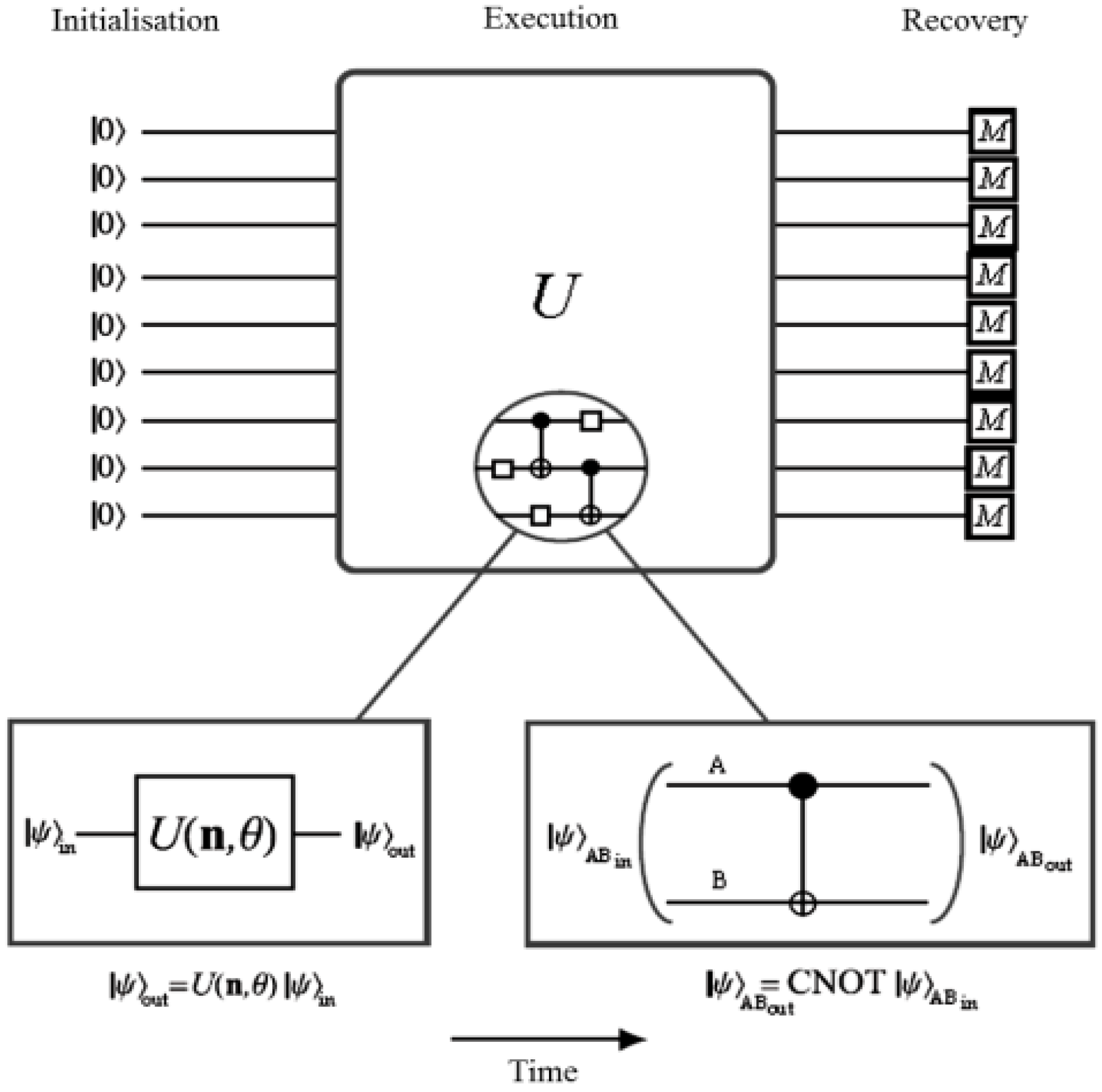
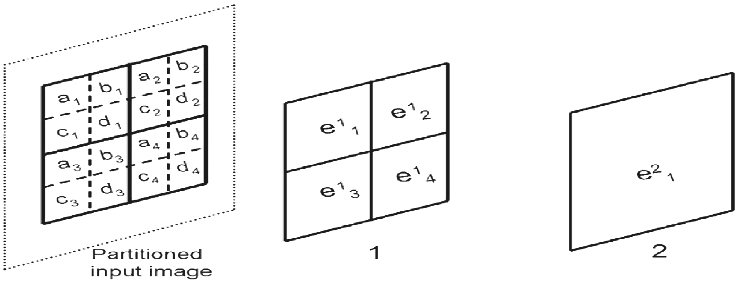
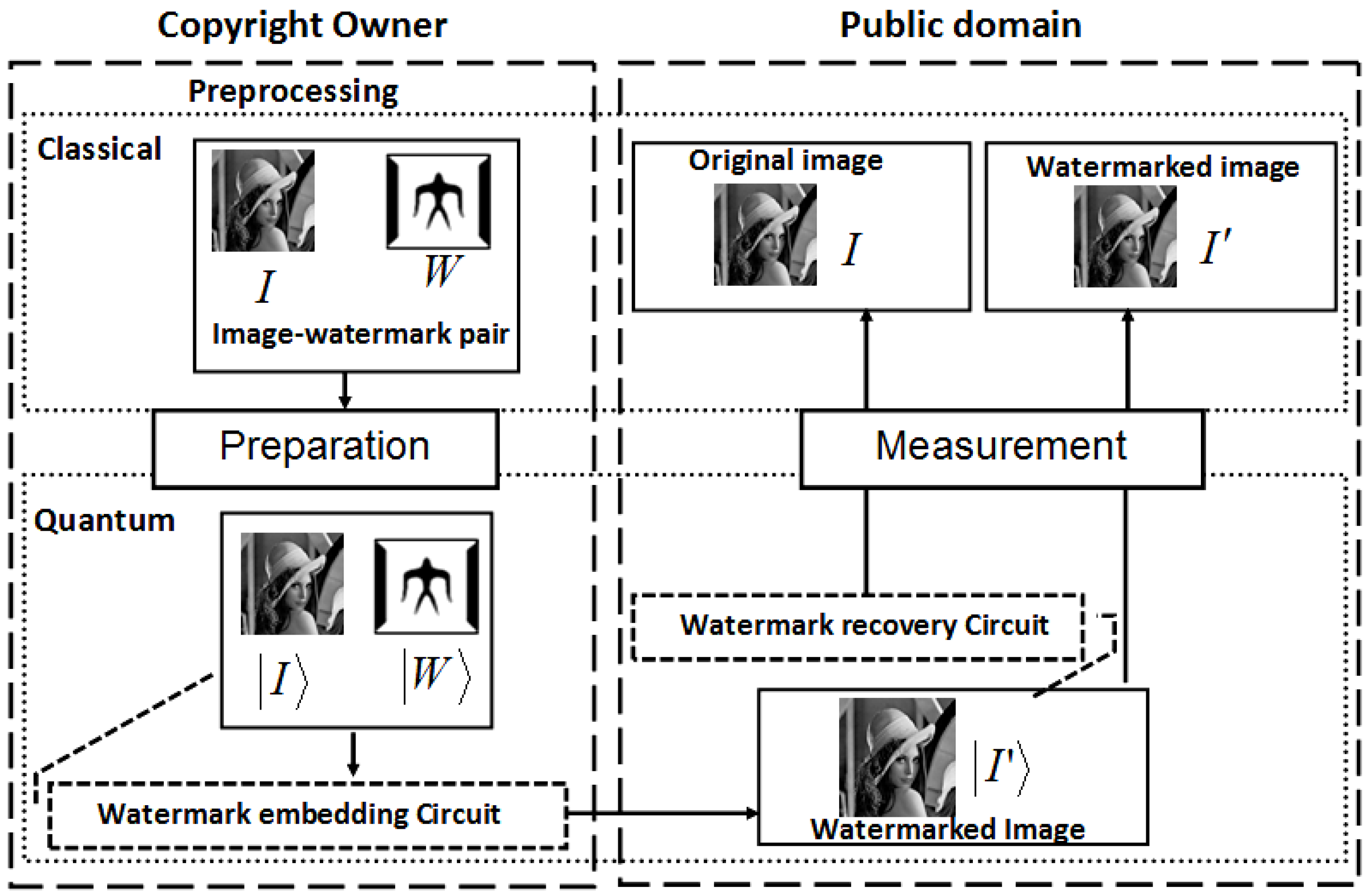
Our proposed application to represent and produce quantum movies allows us generalise some of these criteria. Accordingly, we propose to merge the first three requirements to specify the preparation of the system. By this we mean a scalable physical quantum state that has been initialised and is capable of exhibiting all the inherent properties of a quantum mechanical system such as decoherence, entanglement, superposition, etc. The next requirement specifies that, a state so prepared can only be manipulated by a sequence of quantum gates. Intuitively, we refer to this requirement as manipulation of the quantum system. Finally, the last requirement—measurement, allows us to retrieve a classical read out (observation or measurement) of the quantum register which yields a classical-bit string and a collapse of the hitherto quantum state. Throughout the remainder of this section, by measurement we mean non-destructive measurement, whereby the quantum state is recoverable upon the use of appropriate corrections and ancillary information. Our earlier assumptions that the quantum computer is equipped with in-built error correction and that the classical input images (in this case movie frames) are used to prepare their quantum versions; and that the two are exact replicas of one another are also tenable for the proposed quantum movie framework.

The conceit backing our generealisation of Divincenzo’s criteria, and therefore the proposed framework, hinges on the assumption that it is possible to realise standalone components to satisfy each of the aforementioned criteria, and that the components can interact with one another as does the CPU, keyboard, and display (monitor) units of a typical desktop computer.

The UQC paradigm for implementing quantum algorithms, in which the algorithms are compiled into a sequence of simple gates acting on one or more qubits, is adopted for the manipulation criteria of the proposed framework [19]. Many of these quantum algorithms are expressed in terms of uniform special-purpose circuits that depend strongly on the problem at hand [4,19]. These circuits comprise various levels of abstraction and combinations of the universal gates: NOT (N), controlled-NOT (C), and the Toffoli (T) gates as reviewed in preceding sections. These gates combine to form what is often referred to in the literature as the NCT library [4,18,19,29].

Recently, applications aimed at exploiting the versatility of quantum circuit modeling of quantum gates in quantum image processing have started gaining ground. As reviewed in Section 2, Le et al. [30] adopted the FRQI representation proposed in [11,12], to explore the formulation of a special group of classical-like geometric transformations such as flip, coordinate swap, two-point swap, and rotation on quantum images, this was christened as geometric transformations on quantum images (GTQI). A trio of strategies to design these geometric transformations for manipulating FRQI images was proposed in [1,31]. Using restricted versions of these transformations [1,17,18] to target smaller regions of the images, the possibility of using two or more quantum images to produce a single quantum circuit that could be used in order to accomplish the watermarking, authentication and recovery of FRQI quantum images was explored in [18,20] as reviewed in Section 4 and Section 5.

The framework proposed in this section builds on these various literatures by extending the classical movie applications and terminologies toward a new framework to facilitate movie representation and production on quantum computers.

Classically (on traditional or non-quantum systems), a movie comprises a collection of multiple images, and every such movie was at some stage a script, i.e. merely a collection (usually in writing) of various predetermined dialogues and instructions required to convey a storyline to the audience. In order to convey this larger narrative of a movie, four levels of detail are required [19,65]. At the lowest level, a movie consists of a set of almost identical images called frames, which at the next level are grouped into shots. Each shot is delineated by two or more frames that exhibit very little resemblance to each other called key frames [19,65]. Consecutive shots are then aggregated into scenes based on their pertinence. A scene could have a single shot, and usually all the shots in a single scene have a common background. A sequence of all scenes together composes a movie. Various people are involved at different stages of making a movie. To breathe life into the script, the director translates its content into the various levels of the movie as enumerated earlier on. To accomplish this, he relies on different personnel some of which are visible in the movie — the cast, and others (the crew) who although not visible in the final movie are indispensable toward its realisation.

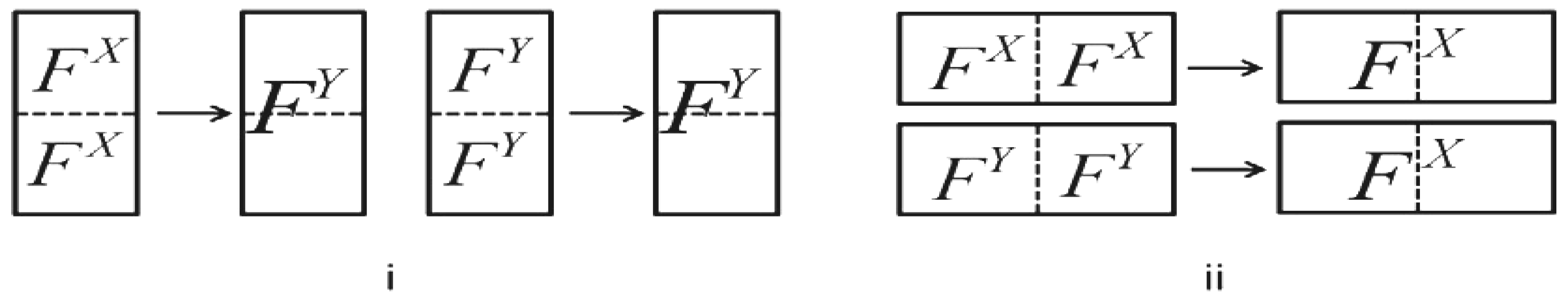
These classical terminologies and roles are extended to the proposed representation and production of movies on quantum computers. The inherent nature of quantum computers, however, imposes the need for the services of an additional professional whom we shall refer to as the circuitor. His responsibilities complement that of the director, in that, he is saddled with choosing appropriate circuit elements to transform each key frame into a shot (or part thereof), so as to combine with others in order to convey the script to the audience. Alternatively, this role could be added to the director of a quantum movie in addition to his traditionally classical duties.

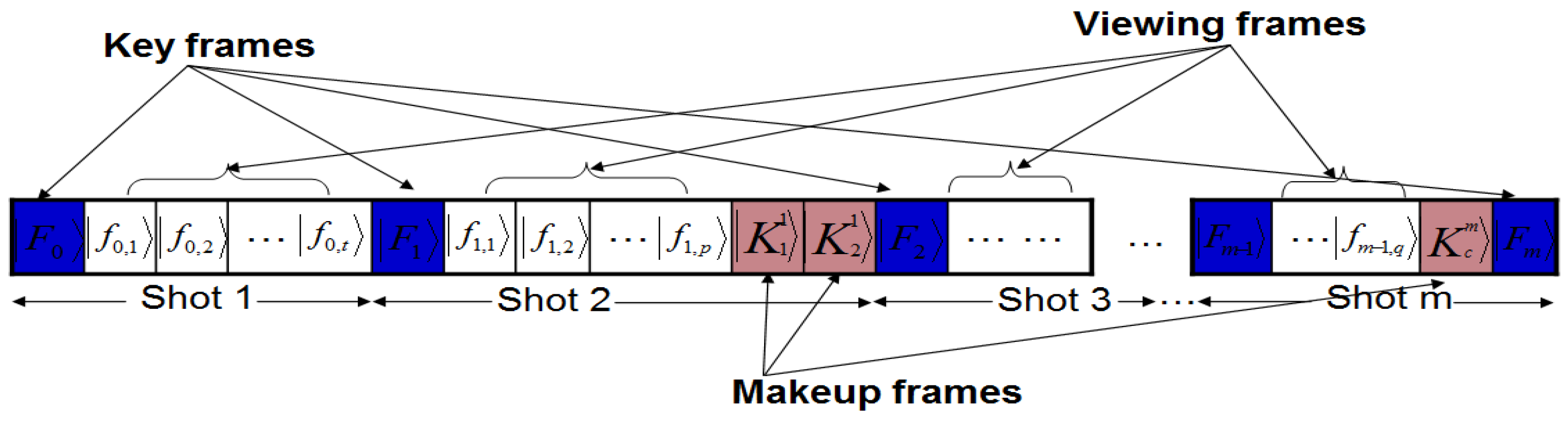
In line with these abstract requirements to represent a movie, we propose a conceptual device or gadget to encompass each of our generalised broad requirements for quantum computing, i.e. preparation, manipulation, and measurement. Accordingly, we propose a compact disc — CD (or cassette) — like device to store the most basic information of the proposed framework, the key frames. Our proposed device, which we shall refer to as the quantum CD, has the additional capability to prepare, initialise, and store as many key frames and their ancillary information as required for the various scenes of the movie. The transformed version of each key frame at every layer of the circuit produces a viewing frame: which is a frame that is marginally different from the frame content at the previous layer. This vastly interconnected circuit network is housed in a single device which we refer to as the quantum player in analogy with the classical CD (VCD, DVD, or VCR) player. The combination of two extreme key frames and the resulting viewing frames to gradually interpolate between them produces a sequence, which conveys a scene from the movie. The last device required to facilitate the representation and production of our quantum movies is the movie reader. As the name suggests, this device measures the contents of the sequence (comprising of the key, makeup, and viewing frames) in order to retrieve their classical readouts. At appropriate frame transition rates, this sequence creates the impression of continuity as in a movie.

The trio of the quantum CD, player, and movie reader, albeit separate, combine together to produce our proposed framework to represent and produce movies on quantum computers.

Succinctly put, the main contributions of this work include proposing the following:

• An architecture to encode multiple images (key frames) as a single coherent superposition of the key frames called the strip. This is prepared, stored, and initialised in the quantum CD.
• Operations to transform the content of each key frame in order to convey a part of the movie. These operations transform the key frame in order to produce an unbroken sequence of frames needed to depict simple 2D motion operations such as walking, running, jumping, or movement about a circular path according to the script.
• A frame transition operation to allow for seamless transition from one frame to another and facilitate classical-like playback/forward operations on the quantum video. These operations together with those in (ii) are processed by the quantum player.
• A classical system to recover the readout of the sequence comprising of the key frames and the new viewing frames realised from their transformation using the movie reader.

In addition to these technical advances, the likely challenges to pioneer representing and producing movies on quantum computers are reviewed. This will facilitate the exploitation of the proven speedup of quantum computation by opening the door towards practical implementation of quantum circuits for information representation and processing.

6.1. The Quantum CD

The first step in representing a movie is being able to capture the key frames that represent the broad content or scenes of the movie. This section discusses how to represent and encode a single key frame and multiples of such frames into a single representation that can be further processed as dictated by the movie script. The device to encode, capture, and store 2m multiple key frames, each a 2ⁿ × 2ⁿ frame (FRQI image) is referred to as the quantum CD. The FRQI representation for quantum images including its preparation was reviewed in Section 2 and discussed thoroughly in [1,11,12].

6.1.1. Movie Representation Based on the FRQI Representation

Movies comprise of multiple images (frames) that include slight changes from one frame to the next which combine to produce a single shot. Conveying these changes effectively depends on the appropriate choice of the representation used to encode the content of the key frame so that it allows the use of specific transformations. In addition, such a representation should also be flexible enough to isolate a smaller region of interest (ROI) within a key frame in order to depict smaller operations as dictated by the movie script. In addition to this ability to isolate a smaller ROI, the representation we seek should possess two additional features: the geometric (position) and visible (colour) information of every point in that frame. As earlier introduced earlier, the FRQI representation exhibits these three properties [38], and is, hence, sufficient for representing a single key frame. The overall requirements of a movie, however, transcend a single frame. Hence, in order to accomplish the effective representation and production of a movie on a quantum computer, a representation capable of capturing the content of each key frame individually and a combination of these key frames as required for each particular scene of the movie is essential. In the remainder of this section, we shall restrict our reference to an FRQI image to mean a key frame or vice versa. In either case, a constant background, binary image is implied. In the ensuing discussion, such a binary image will be characterised by two binary levels, black and white. While restricted in application, such images are of interest because they are relatively straightforward to process and therefore provide a useful starting point for recovering the images that yield our quantum movie. Hence, we assign a state $|0\rangle$ to every white point on the 2D grid, while a black point corresponds to a state $|1\rangle$.

We begin discussion on our proposed quantum CD with some clarifications that will aid in distinguishing between a key frame and another type of frame — the makeup frame, which together form the main building block of the quantum CD, the movie strip, and to some extent the entire framework.

Definition 1: A key frame is an FRQI quantum image state as defined in Equation (1) that captures the broad content from which the additional information required to convey a single shot (or a part of it) in a movie is obtained.

The ingenuity of the quantum CD lies in the use of quantum circuit elements to interpolate the missing content that connects the shots in the hitherto abstract or summarised version of the movie, i.e. the script. Each shot is characterised by at least a single key frame, the last of which could signal both the end of a preceding shot and the start of the present one. In conveying the content of a movie, the transition of its content is gradual both in the change to depict motion (or movement) and in time. When one or more key frames are set, the motion (as dictated by the movie script) generates the in-between frames, resulting in a smooth change of the content over time. Moreover, key frame representation is a simple, yet effective way for summarising the content of video for content browsing and retrieval [19,65]. The in-between or missing content realised from each key frame called viewing frames soften the hitherto abrupt transition from one key frame to another. Where a scene in a movie cannot be adequately conveyed by transforming a preceding key frame, the third type of frame — the makeup frame is prepared and included in the movie sequence. The main difference between a key frame and a makeup frame is that viewing frames cannot be realised from a makeup frame. In other words, makeup frames do just that — they make up for missing content within the movie sequence.

Figure 45. m-shots from a movie showing the key |F_m〉, makeup $|K_c^m\rangle$, and viewing |F_mq〉 frames.

Figure 45. m-shots from a movie showing the key |F_m〉, makeup $|K_c^m\rangle$, and viewing |F_mq〉 frames.

Within a movie sequence, however, a makeup frame can only be preceded or succeeded by a key frame or another makeup frame. Very often, especially, where their distinction from key frames is essential, we shall refer to makeup frames as $|K_c\rangle$. To conclude, we emphasise that irrespective of its type, i.e. key, viewing, or makeup, all the frames are FRQI quantum states as defined in Equation (1). Figure 45 outlines the proposed schematics for the three types of frames as explained.

Without loss to the generality conveyed earlier and with reference to their presence in the strip we shall often refer to the combination of the key and makeup frames for the nth shot as simply the key frames of that shot. The key (and makeup) frames are encoded into a collection of 2^m-ending frames as required to capture the information necessary to represent higher levels of the movie, i.e. the shots and scenes as discussed in earlier in this section. This representation referred to here as the movie strip or simply a strip is presented in Definition 2. The circuit structure to encode this representation shall be referred to as the movie FRQI or simply mFRQI.

Definition 2: A strip $|S\left(m,n\right)\rangle$ is an array comprising of a collection of $2^m$—ending key (and makeup frames) each a 2ⁿ×2ⁿ FRQI quantum image state defined as follows:

$$|S\left(m,n\right)\rangle =\frac{1}{2^m}{\displaystyle \sum _{j=0}^{2^m-1}|F_j\rangle \otimes |j\rangle }$$

(46)

where:

$$|F_j\rangle =\frac{1}{2^n}{\displaystyle \sum _{i=0}^{2^{2n}-1}|c_{j,i}\rangle \otimes |i\rangle }$$

(47)

Here, $|c_{j,i}\rangle$ is the colour of the jth key frame, i is the position of that point in the frame as defined in Equation (47), m is the number of qubits required to encode the spatial information about the entire strip $|j\rangle$, and n is the number of qubits required to encode each key (or makeup) frame.

As seen in Figure 46, the depth (in this case the size of the strip) of the mFRQI representation, i.e. the circuit, to capture the input state of the movie strip comprising 2^m key (and makeup) frames increases with the number of such frames. This strip is the input state of the quantum CD after its initialisation and depending on the location of the strip, S-axis; the resulting strip could be interpreted as being horizontally or vertically oriented.

To summarise, each frame (whether key or makeup) is an FRQI state while any combination of multiple key (and makeup) frames—a strip, is best represented as an mFRQI state.

In addition to the 2m—ending key (and makeup) frames captured and stored as discussed earlier in this section, information that loosely pertains to the colour of every pixel in each frame is stored. This ancillary information can be recovered from the script and the preparation of the key (and makeup) frames. In its most simple form, this information specifies that a pixel has a fill or not which corresponds to |0〉 and |1〉, respectively. Each key (or makeup) frame requires 2ⁿ×2ⁿ ancillary information in order to determine which part is filled (not minding its colour) or not. This ancillary information forms the cornerstone on which the dependent ancilla-driven movie reader presented in later parts of this section is based.

Figure 46. Circuit structure to encode the input of a movie strip.

Figure 46. Circuit structure to encode the input of a movie strip.

6.1.2. Initialising a Movie Strip

Whatever the technology chosen for implementing the proposed framework, the information encoded by the resulting qubit, be it a photon, an electron, an atom, or a molecule with certain spin state, can be used to store visual information [9,19]. Combined with other information, an entangled state comprising multiple pixels, which in its most generalised form is defined in Equation (1) is realised [19,42]. The quantum register, i.e. the strip, comprising multiple such images is of the form defined in Equation (46). This strip of length m comprising the collection of 2^m—ending key (and makeup) frames is then initialised by placing the frames in a superposition where each basis state is equally probable. Theorem 3 presents the requirements in terms of the basic gates for preparing a movie strip.

Theorem 3 (Movie Strip Preparation Theorem) The number of operations to transform a quantum player from the initialised state ${|0\rangle }^{\otimes m+2n+1}$ to the mFRQI state in Equation (46) comprises a bivariate (in terms of the size of each key frames n, and the number of these key (and makeup) frames in the strip m) polynomial number of simple gates.

Proof: From Lemma 1, Corollary 1, and Theorem 1 in [11,12] and Ref. 18, the preparation of a quantum computer from the initialised state to the FRQI state (i.e. a single key (or makeup) frame) requires a polynomial number of simple gates to accomplish. Extending this for 2^m such key (and makeup) frames (required for the mFRQI (strip) state) results in a bivariate polynomial number of simple gates. This number of basic gates is bivariate in terms of the size of each key (or makeup) frame n, and the number of these key (and makeup) frames in the strip m.

Like the preparation step of the physical implementation of most quantum systems, there are numerous challenges that may impede the realisation of the quantum CD as proposed. In spite of these challenges, the optical-based implementation having witnessed a spurt of attention backed with interesting results for various physical implementations in recent times appears a very likely technology to realise our quantum CD. This is because it allows for easy connection of the quantum logic gates and quantum memory using optical fibers or waveguides, analogous to the wires in conventional computers [66,67,68]. This offers modularity that is not readily available in other approaches (technologies) [67,68]. For example, the transfer of qubits from one location to another in ion-trap or NMR systems is a very complex process [1,14,19,66].

An optical mode is a physical system whose state space consists of superpositions of the number of states $|n\rangle$, where $n=0,\hspace{0.17em}1,\hspace{0.17em}\cdots$ gives the number of photons in the mode [19,69]. The initial state is the vacuum state $|0\rangle$ in which there are no photons in any of the modes to be used [68,70]. The basic element that adds photons to the initial state is the single photon source. It can be used to set the state of any given mode to the one-photon state $|1\rangle$. It is sufficient to be able to prepare this state non-deterministically [19,69]. This means that the state preparation has a non-zero probability of success, and whether or not it succeeded is known. The simplest optical elements are phase shifters and beam splitters [6,19,66,67]. These elements generate evolutions implementable by passive linear optics. In our opinion, these uncomplicated correlations make the optical-based implementation an ideal fit for implementing the proposed quantum CD.

6.2. The Quantum Player

As proposed earlier in this section, the movie strip representation comprising the key (and makeup) frames encodes information that represents an abstract summary of the entire movie. Therefore, transitions from one key (or makeup) frame to the next are at best abrupt and may not effectively convey the storyline as specified by the script. Hence, there is the need to smoothen the abruptness of the content conveyed by the two key frames by way of intercalating the missing content between successive key frames, and a connection between all of these contents, i.e. the key frames and their interpolated content, into a single continuous sequence. The main objective of the quantum player is to manipulate the content of each key frame as required to realise viewing frames which capture the required motion or activity in that shot. It is analogues to the central processing unit of the proposed framework. The script dictates how these key frames are manipulated using the appropriate quantum circuit elements in the quantum player.

A successful representation for a movie based on quantum computation must be capable of showing the movement of an object (or objects) from one frame to another.

This movement should not only be in a single key frame, but it should also be confined within a smaller specified region of the key frame, i.e. an ROI. This section proposes various circuits for representing relative changes in the position of the geometric contents of 2D quantum images as required to effectively depicting the motion. It was shown in [17,19,30,32] that using the FRQI representation, geometric transformations on quantum images is both possible and efficient. In conveying certain parts of the script, we may have to manipulate the chromatic (colour) content of the key frames, and in others, information about both the colour and position must be transformed. Consequently, in addition to transformations focused on manipulating the geometric information of the frames, some of our proposed movie operations will include transformations that target the colour content of the frames (FRQI quantum images) [19,32]. All of these operations and the new ones proposed in this section can apply to the mFRQI representation. In order to specify the key frame, however, it is mandatory to impose additional control on the entire strip coordinate. In addition to reviewing the aforementioned transformations, the sequel introduces the necessary extensions to the geometric and colour transformations in order effectively convey the content of the movie to the audience. The device housing the circuitry to undertake these transformations is referred to as the quantum player.

Geometric and colour transformations on FRQI quantum images together with their restricted versions were reviewed in preceding sections of this review. Relying on the movie script, the circuitor will employ these transformations as the core resources to manipulate the prepared and initialised content of the movie. These resources as needed to translate the bits and pieces of the movie script are discussed in the sequel.

6.2.1. Two-dimensional Motion in a Quantum Movie Key Frame

In any movie representation, depicting the different movements of the various objects which combine to convey the script of the movie to the audience is of paramount importance. In this regard, operations to effectively convey 2D movement of every point (or collectively every object as an entangled state [35,71]) in a quantum movie are necessary. This section proposes various transformations to allow us depict 2D movement of a ROI in a key frame. We start by defining the general position shifting operation in a single key frame.

Definition 3: A simple motion operation (SMO), on an FRQI key frame is an operation S that shifts every point in that frame defined as:

$$S_{c,2n}|i\rangle =|i^{\prime }\rangle ,\hspace{0.17em}\hspace{0.17em}\hspace{0.17em}\hspace{0.17em}\hspace{0.17em}\hspace{0.17em}i\in 0,\hspace{0.17em}1,\hspace{0.17em}\dots ,\hspace{0.17em}{y}_0,\hspace{0.17em}{x}_0,\hspace{0.17em}{x}_1,\hspace{0.17em}\dots ,\hspace{0.17em}{2}^{2n-1}$$

where $i^{\prime }=i+c\mathrm{mod}{2}^{2n}$ and $c\in \hspace{0.17em}\left\{\hspace{0.17em}1,\hspace{0.17em}\dots ,\hspace{0.17em}{2}^{2n-1}\right\}$ called the shift steps is used to indicate the number of steps every point is shifted.

Definition 3 can be decomposed in terms of simple motion operations along the horizontal axis as the forward or backward motion operations denoted as $M_F^c$ and $M_B^c$, respectively. Similarly, along the vertical axis we obtain the upward and downward motion operations, $M_U^c$ and $M_D^c$, respectively. The equations and corresponding circuits to execute these operations are presented in Equations (48)–(51) and Figure 47, respectively.

Starting with the forward and backward SMOs, the modified equations are given as:

$$\begin{array}{l}{M}_F^c|Y\rangle |X\rangle =I|Y\rangle \otimes S_{c,n}|X\rangle ,\\ \hspace{0.17em}\hspace{0.17em}\hspace{0.17em}\hspace{0.17em}\hspace{0.17em}\hspace{0.17em}\hspace{0.17em}\hspace{0.17em}\hspace{0.17em}\hspace{0.17em}\hspace{0.17em}\hspace{0.17em}\hspace{0.17em}\hspace{0.17em}\hspace{0.17em}\hspace{0.17em}\hspace{0.17em}=|Y\rangle |X+c\mathrm{mod}{2}^n\rangle .\end{array}$$

(48)

And the SMO, c steps backward is defined as:

$$\begin{array}{l}{M}_B^c|Y\rangle |X\rangle =I|Y\rangle \otimes S_{-c,n}|X\rangle ,\\ \hspace{0.17em}\hspace{0.17em}\hspace{0.17em}\hspace{0.17em}\hspace{0.17em}\hspace{0.17em}\hspace{0.17em}\hspace{0.17em}\hspace{0.17em}\hspace{0.17em}\hspace{0.17em}\hspace{0.17em}\hspace{0.17em}\hspace{0.17em}\hspace{0.17em}\hspace{0.17em}\hspace{0.17em}=|Y\rangle |X-c\mathrm{mod}{2}^n\rangle .\end{array}$$

(49)

Similarly, along the vertical axis we define the upward and downward SMOs given as:

$$\begin{array}{l}{M}_U^c|Y\rangle |X\rangle =S_{c,n}|Y\rangle \otimes I|X\rangle ,\\ \hspace{0.17em}\hspace{0.17em}\hspace{0.17em}\hspace{0.17em}\hspace{0.17em}\hspace{0.17em}\hspace{0.17em}\hspace{0.17em}\hspace{0.17em}\hspace{0.17em}\hspace{0.17em}\hspace{0.17em}\hspace{0.17em}\hspace{0.17em}\hspace{0.17em}\hspace{0.17em}\hspace{0.17em}=|Y\rangle |X+c\mathrm{mod}{2}^n\rangle ,\end{array}$$

(50)

and

$$\begin{array}{l}{M}_D^c|Y\rangle |X\rangle =S_{-c,n}|Y\rangle \otimes I|X\rangle ,\\ \hspace{0.17em}\hspace{0.17em}\hspace{0.17em}\hspace{0.17em}\hspace{0.17em}\hspace{0.17em}\hspace{0.17em}\hspace{0.17em}\hspace{0.17em}\hspace{0.17em}\hspace{0.17em}\hspace{0.17em}\hspace{0.17em}\hspace{0.17em}\hspace{0.17em}\hspace{0.17em}\hspace{0.17em}=|Y\rangle |X-c\mathrm{mod}{2}^n\rangle ,\end{array}$$

(51)

respectively, where I is an identity operation.

From the figures in Figure 47 we notice that the circuit on the left (in Figure 47) has $C^{n-1}\left({\sigma }_x\right)$ controlled-NOT gates on the first layer and $C^{n-2}\left({\sigma }_x\right)\cdots C\left({\sigma }_x\right)$ controlled-NOT gates, ${\sigma }_x$, along the remaining layers. In contrast, the circuit on the left (in the same Figure 47) has $C\left({\sigma }_x\right)$, i.e. a NOT gate, on its first layer and $C^{n-2}\left({\sigma }_x\right)\cdots C\left({\sigma }_x\right)$, ${\sigma }_x$ along its remaining layers. Applied along the vertical axis, the circuits (on the left and right in Figure 47) produce the $M_F^c$ and $M_D^c$ SMOs, respectively. Similarly, applied along the vertical axis the same circuits yield the $M_B^c$ and $M_U^c$ SMOs as defined earlier.

Figure 47. Circuit structure to encode the input of a movie strip Circuits for SMO. Depending on the motion axis Z_n = x or y) the circuit on the left is used to accomplish the $M_F^c$ and $M_D^c$ operations when applied along the x⁻ and y⁻ axis, respectively. Similarly, the circuit on the right is used to accomplish the $M_B^c$ and $M_U^c$ operations when applied the x⁻ and y⁻ axis, respectively.

Figure 47. Circuit structure to encode the input of a movie strip Circuits for SMO. Depending on the motion axis Z_n = x or y) the circuit on the left is used to accomplish the $M_F^c$ and $M_D^c$ operations when applied along the x⁻ and y⁻ axis, respectively. Similarly, the circuit on the right is used to accomplish the $M_B^c$ and $M_U^c$ operations when applied the x⁻ and y⁻ axis, respectively.

The resulting effects of applying the $M_F^c$ and $M_U^c$ SMOs on the “+” shaped ROI (which takes up three pixels along each axis) in Figure 48(a) are presented in Figure 48(b) and (c), respectively. As prepared in this figure, applying the $M_F^c$ and $M_U^c$ avails the +-shaped ROI of only three and five available shift steps along the horizontal and vertical axis respectively. In terms of mFRQI quantum movie nomenclature, we say that only three and five viewing frames are realisable from the + shaped key frame Figure 48(a).

Consequently, the number of viewing frames realisable from a key frame depends on:

• The size of the key frame;
• The size of the ROI targeted by the script; and
• The content of the script, i.e. the specific actions being depicted

Applying a SMO operation on a key frame arbitrarily, results in a situation called an overflow. In such a situation, a viewing frame wherein part or all the pixels of the ROI appear disjointed from the rest of the ROI in tandem with the operation performed on the key frame is realised. An example of this phenomenon is demonstrated in the last viewing frames from the sequences in Figure 48b and c. As seen from the content of these frames, if overflows are left unchecked they enervate the content of the script, often eroding or misrepresenting the intended dialogue being conveyed. The overflow can be smoothened in order to depict certain actions such as back and forth movement by an ROI by adjusting the shift steps c. The last two viewing frames for the zigzag motion of the + shaped ROI in Figure 48d demonstrate how overflow can be avoided by adjusting the shift step between them to c=3.

Figure 48. SMOs on the key frame in (a) to mimic the movement of the + shaped ROI on a constant white background and its viewing frames after applying (b) the forward motion operation $M_F^c$, (c) the upward motion operation $M_U^c$, and (d) a somewhat zigzag movement of the + ROI.

Figure 48. SMOs on the key frame in (a) to mimic the movement of the + shaped ROI on a constant white background and its viewing frames after applying (b) the forward motion operation $M_F^c$, (c) the upward motion operation $M_U^c$, and (d) a somewhat zigzag movement of the + ROI.

Definition 4: On a 2ⁿ × 2ⁿ FRQI key frame, the displacement operation, 2ⁿ×2ⁿ to shift the position of every pixel in the entire key frame (or any part, an ROI, thereof) c and d steps along the horizontal and vertical axis respectively can be defined as:

$$V_D^{c,d}|Y\rangle |X\rangle =|Y\pm c\mathrm{mod}{2}^n\rangle \otimes |X\pm d\mathrm{mod}{2}^n\rangle ,$$

(52)

where D indicates the nature of the final displacements for c and d shifts along the horizontal and vertical axis respectively, and $c,d\hspace{0.17em}\in \left\{0,\hspace{0.17em}1,\cdots ,\hspace{0.17em}{2}^{2n-1}\right\}$. Such operations are realised via different combinations of the SMOs defined in Equations (48)–(51).

These SMO operations can be combined with the GTQI operations [30,31] in order to realise any 2D motion as would be required in a movie. In other instances, we may need to use the CTQI operations [32] to do so. As stated in Definition 4, SMO operations can be combined to realise more complex operations that displace part or all the content of a key frame in order to convey different actions. The somewhat zigzag movement of the + shaped ROI in Figure 48(d) was obtained by combining the $M_F^c$ and $M_U^c$ SMO operations.

We shall refer to this enhanced library comprising of the SMO operations discussed here and the GTQI and CTQI operations as simply movie operations. To illustrate parts of a movie utilising combinations of these movie operations, we consider a constant background two-scene movie in the example in Figure 49. The movie script Figure 49(a) specifies in scene 1 that an object R1 moves through the nodes labelled 0-8 in the direction shown by the arrows in this figure. For exigency, we impose an additional requirement that in moving through its defined trajectory, R1 can only merge diagonally with any of the pixels from a letter “a” formed by transforming the pixels in the first three columns of the key frame. This movement of R1 while avoiding the letter “a” continues up to node 5. In the second scene, the script dictates that from node 6 to node 8 the movie has a second ROI R2. Together with this new ROI, our object R1 continues its journey from node 5 to node 8. R2 has a motion path indicated by the arrows connecting the nodes labelled 5′, 6′, 7′and $8^{\prime }$ as shown in Figure 49(b). In the sequel, we discuss the abstract and detailed requirements of each scene separately. Similarly, for brevity, we conclude by showing the movie sub-circuit for each scene separately.

Scene 1: Each of the paths connecting the nodes in the movie sub-script for this scene in Figure 48(a) is conveyed using an SMO operation. To effectively convey the additional letter “a” constraints imposed on the movement of R₁ through the nodes 1-4, however, appropriate choices of the CTQI operations as discussed earlier must be used. Combined together, these circuits (comprising the SMO and CTQI operations) form the movie sub-circuit for this scene labelled as sub-circuit 1(a) and 1(b), respectively, in the movie circuit in Figure 50. This is the movie sub-circuit to metamorphose the content of the key frame in Figure 49d in order to translate this script (directions and sequences which add up to produce motions and actions) as presented in Figure 49.

In order to, first of all, perform the predetermined SMO operation ($M_F^c$) that shifts the ROI from node 0 to node 1 as specified by the script, our focus is on the upper-right half of the original image. This corresponds to the 2×2 sub-area shown on the right in Figure 51.

This operation is accomplished by the first layer of the movie circuit which is labelled as sub-circuit 1(a) Figure 50 and is realised using the steps enumerated below.

• Assign a control operation on qubit $y_1=0$. This divides the key frame into two halves: the right and left half. Our ROI being in the right half makes this half our target;
• Assigning another control operation on qubit $x_1=0$ further divides the right half into two halves (each a quarter of the original image): the upper and lower right half, respectively;

Finally, we assign the predetermined movie operation (in this case an $M_F^1$ operation) on qubits $y_0$ and (or) $x_0$ as required for the operation.

Figure 49. Movie scenes to demonstrate SMO operations. The panels in (a) and (b) show the transcribed scripts for scene 1 and 2, (c) shows the key frame for scene 1, and (d)-(l) show the resulting viewing frames.

Figure 49. Movie scenes to demonstrate SMO operations. The panels in (a) and (b) show the transcribed scripts for scene 1 and 2, (c) shows the key frame for scene 1, and (d)-(l) show the resulting viewing frames.

Using the restrictions listed above, the $M_F^c$ operation on the x0 qubit in the first layer of our movie circuit (Figure 50) transforms our ROI from position $|00\rangle$ to $|01\rangle$ within the 2 × 2 sub-area of the key frame for our example as simplified in Figure 51. This new position (node 1) serves as input to be transformed by the next movie operation as earlier explained. This successive evolution of the script continues until the operations in all the sub-circuits are performed.

Similar control operations are used on the CTQI operations in order to effectively convey the additional requirements of the sub-script as it pertain to the letter “a” constraints of the script. As prepared, all the pixels in our key frame have their colour $|c_i\left(\theta \right)\rangle$ defined as in Equation (2) with $\theta =0$ for our ROI and $\theta =\frac{\pi }{2}$ in all the other pixels. Having known beforehand the position of R₁ at each instance, the circuitor in liaison with the director can satisfy the additional requirements (letter “a” constraints) of this subscript by using the restricted versions of the CTQI transformations discussed in Section 3.

The combined effect of applying sub-circuit 1 on the key frame as measured by $M_0^1$ (a sub-circuit of the movie reader) is the viewing frame $f_{0,1}$ shown in Figure 49(e). Employing similar techniques, we realise the movie sub-circuit for this scene as presented in Figure 50. Each path connecting two nodes is conveyed using an SMO (and often GTQI) operation. Thus, this script requires q = 8 sub-circuits (i.e. the number of nodes) to translate. These sub-circuits vary in complexity and number of layers especially when the additional letter “a” constraints are considered. However, for brevity, we restrict the circuit to show only operations required to realise the viewing frames of the first three nodes. The measurements $M_1^0$, $M_2^0$ and $M_3^0$ in Figure 50 produce the viewing frames $f_{0,1}$, $f_{0,2}$ and $f_{0,3}$ shown in Figure 49(e) to (g).

Figure 50. Movie sub-circuit to realise the first three viewing frames of scene 1 (of the example in Figure 49). The layers separated by short-dashed lines labelled “a” indicate SMO operations, while the layers grouped and labelled as “b” indicate CTQI transformations on the key frame. Layers labelled $M_1^2$, $M_2^0$ and $M_3^0$ indicate sub-circuits of the movie reader to recover the classical readout of frames |f_0,1〉, |f_0,2〉 and |f_0,3〉.

Figure 50. Movie sub-circuit to realise the first three viewing frames of scene 1 (of the example in Figure 49). The layers separated by short-dashed lines labelled “a” indicate SMO operations, while the layers grouped and labelled as “b” indicate CTQI transformations on the key frame. Layers labelled $M_1^2$, $M_2^0$ and $M_3^0$ indicate sub-circuits of the movie reader to recover the classical readout of frames |f_0,1〉, |f_0,2〉 and |f_0,3〉.

Figure 51. Restricting the movie operation $M_F^C$ in order to move the ROI R₁ from node 0 to node 1 as specified by the movie script.

Figure 51. Restricting the movie operation $M_F^C$ in order to move the ROI R₁ from node 0 to node 1 as specified by the movie script.

Scene 2: The sub-script for this scene specifies that while R1 continues its movement along the path shown in Figure 49(a) (the script), we are required to track the movement of another object, R2, through the nodes labelled $5^{\prime },\hspace{0.17em}{6}^{\prime },\hspace{0.17em}{7}^{\prime },\hspace{0.17em}$ and $8^{\prime }$ as shown in Figure 49(b). We assume a node-by-node movement for both objects, i.e. R₁ moves first from node 5 to node 6 and is then followed by R2’s movement from node 5′ to node 6′ and so on in that fashion, in order to create the impression of simultaneous movement of R₁ and R₂. To accomplish this, we have the option of using restricted versions of the CTQI operations as in scene 1, or alternatively, we could assume a second key frame is prepared with R₁ and R₂ in the locations specified as node 5 and 5′, respectively as shown in Figure 49(c).

Figure 52. Movie sub-circuit for scene 2 in Figure 49(b). The labels 5 through 7 and 5′ through 7′ for R₁ and R₂ indicate the circuit layers to perform the operations that yield the viewing frames in Figure 49(j) –(l).

Figure 52. Movie sub-circuit for scene 2 in Figure 49(b). The labels 5 through 7 and 5′ through 7′ for R₁ and R₂ indicate the circuit layers to perform the operations that yield the viewing frames in Figure 49(j) –(l).

Using appropriate control-operations as discussed earlier, the motion paths of the two objects can be effectively separated and the sequence of the SMO operations to realise them can be altered in order to convey the simultaneous movement of R₁ and R₂ as dictated by the sub-script. The movie sub-circuit for this scene is presented in Figure 52. Similar to the sub-circuit in scene 1, each of the measurements $M_1^1$, $M_2^1$ and $M_3^1$ in Figure 52 produces the viewing frames $f_{1,1}$, $f_{1,2}$ or $f_{1,3}$ in Figure 49(j) to (l).

As seen from the figures presented so far in this section, the effects of the proposed SMOs are restricted to a single key frame. Additionally, we have seen that there could be q such transformations on the key frame. These operations although very important for the success of our proposed framework are still inadequate for effective representation of all the abstract requirements of a movie. In the sequel, we consider operations on the entire mFRQI state, such as those required to facilitate transition from one frame to another.

6.2.2. Frame to Frame Transition

A key advantage of the mFRQI representation is that it allows the use of q different sub-circuits each geared toward accomplishing a certain transformation on a preceding frame. Because of the marginal changes in the content of the realised frames, seamless movement of ROI’s involving movie operations each of which is performed by a sub-circuit is obtained. Where $q=0$, then the transition from one key (viewing or makeup) frame to another, c steps apart, is immediate. To achieve the transition from one frame to the next, we define in Equation (54) the strip transition operation, $T_i^c$ which targets the strip, S-coordinate only.

Definition 5: The frame-to-frame transition operation $T_i^c$ on an mFRQI strip $|S\left(m,n\right)\rangle$ as defined in Equation (46) is the operation used to shift from one key (or makeup) frame to another in a quantum movie:

$$T_i^c|S\left(m,n\right)\rangle =\frac{1}{2^m}{\displaystyle \sum _{j=0}^{2^m-1}|I_j\rangle \otimes }{T}_i^c|j\rangle ,$$

(54)

$$T_i^c|S\left(m,n\right)\rangle =\frac{1}{2^m}{\displaystyle \sum _{j=0}^{2^m-1}|I_j\rangle \otimes }|j\pm c\mathrm{mod}{2}^m\rangle ,$$

(55)

where $c\in \hspace{0.17em}\left\{0,\hspace{0.17em}1,\hspace{0.17em}\cdots ,\hspace{0.17em}{2}^{2n-1}\right\}$ is the shift steps to transit from the $n^{th}$ frame, $|F_n\rangle$, to another frame $|F_{n\pm c}\rangle$, c steps up or down the length of the strip.

Transition from one frame to the next requires $c=1$ shift steps. In addition to aiding smooth transition from frame to frame, Equation (54) allows for repeating a single frame in generating the final frame sequence to be viewed by the audience. This eliminates the need to duplicate the same frame should its need elsewhere within the script arise again. In addition, it allows video processing operations such as playback (or forward). As discussed earlier in this section, the input state (strip) of the proposed framework to represent a quantum movie encodes all the necessary information to specify each key (or makeup) frame $|F\rangle$ and the position of that frame within the larger strip $|S\left(m,n\right)\rangle$. The output of every transformation by a sub-circuit on a single frame produces a single viewing frame, $|f\rangle$. After q transformations on a key frame, the strip transition operation $T_i^c$ is used to adjust to the next frame c steps from the current frame. The circuit to accomplish the strip transition operation $T_i^c$ that enables transition from one frame to the next is applied on the strip coordinate is presented in Figure 53.

Figure 53. Circuit on the mFRQI strip axis to perform the frame-to-frame transition operation.

Figure 53. Circuit on the mFRQI strip axis to perform the frame-to-frame transition operation.

Using the control-operations (on the strip axis) to specify on which key frame to perform a particular movie operation increases the complexity of the new transformation in terms of the depth and the number of basic gates in the corresponding circuit. The general case for adding more than two controls can be realised by an extension of Theorem 1 in [30]. From this, it is trivial that the complexity of position shifting transformation in the worst case is $O\left(n^2\right)$.

Notice that control-operations on the strip (S) axis were used to confine the transformations to the required key frame in the movie sub-circuits in Figure 48 and Figure 52 for scene 1 and scene 2 of the previous example. Without this restriction, all the operations applied thereafter will affect both key frames in the movie, i.e. Figure 49d that was hitherto for scene 1 and Figure 49c. This is a clear example of the use of the frame-to-frame transition operation.

Assuming the script dictates a transformation on the $m^{th}$ key frame that requires q movie operations to accomplish, then a sequence:

$$SMO\hspace{0.17em}|F_m\rangle =|f_{m,0}\rangle ,\hspace{0.17em}|f_{m,1}\rangle ,\hspace{0.17em}\cdots ,\hspace{0.17em}|f_{m,q}\rangle$$

(56)

comprising of q marginally different viewing frames is obtained before transition to the next key (or makeup) frame. This produces a final sequence comprising all the key (and makeup) frames and the viewing frames realised from their transformation as dictated by the movie circuit (script). This sequence, called the movie sequence $|M\rangle$ is shown as follows:

$$\begin{array}{l}|M\rangle =|F_0\rangle \left(|f_{0,0}\rangle ,\hspace{0.17em}\cdots ,\hspace{0.17em}|f_{0,p}\rangle \right)\hspace{0.17em}|K_1^0\rangle |F_1\rangle ,\hspace{0.17em}\cdots ,\hspace{0.17em}\\ \hspace{0.17em}\hspace{0.17em}\hspace{0.17em}\hspace{0.17em}\hspace{0.17em}\hspace{0.17em}\hspace{0.17em}\hspace{0.17em}\hspace{0.17em}\hspace{0.17em}\hspace{0.17em}\hspace{0.17em}\hspace{0.17em}\times |F_2^{m-1}\rangle \left(\hspace{0.17em}|f_{2^m-1,0}\rangle ,\hspace{0.17em}\hspace{0.17em}\cdots ,\hspace{0.17em}|f_{2^m-1m-1,q}\rangle \right)\hspace{0.17em}\hspace{0.17em}|F^{2^m}\rangle .\end{array}$$

(57)

The width of the movie circuit W(C) to generate this sequence depends on the number of key frames (and where required the makeup frames) encoded on the strip and the size of each frame. The depth of the circuit D(C) is a function of the output requirements of the movie, which is determined by the number of layers in each sub-circuit. This is in turn dictated by the movie operations necessary to convey the story in the movie script. It is easy to see that the cost of preparing a quantum movie $\left|C\right|$ is represented by the number of key frames (and makeup frames) required to capture all the major content of the movie, $\left|m\right|$; the size of each of the frames $\left|n\right|$; the total number of movie operations to effectively describe the content of the movie, $Q={\displaystyle {\sum }_{m=0}^{m=2^m-1}}$; and the number of basic gates required for each operation. Figure 54 demonstrates a cyclic shift operation for the case $c=1$ and $n=5$.

Figure 54. The cyclic shift transformation for the case c = 1 and n = 5.

Figure 54. The cyclic shift transformation for the case c = 1 and n = 5.

Like the quantum CD, our intuition for the manipulation of the prepared states leans toward the use of optical devices. Single-qubit gates can be easily implemented physically, for example, by quarter- and half-wave plates acting on polarised photons, or by radio-frequency tipping pulses acting on nuclear spins in a magnetic field [22]. Similarly, two-qubit optical gates, such as a CNOT gate, have been implemented without need for nonlinear interaction between two single qubits [1,19,41,70,72,73,74]. Logic gates of this kind can be constructed using only linear optical elements such as mirrors and beam splitters, additional resource photons, and triggering signals from single photon detectors [66,70,73].

Using appropriate optical elements, numerous quantum gates and algorithms have been simulated and implemented. To mention just a few: the linear implementation of the quantum SWAP gate [73], quantum optical Fredkin gate [72], optical based implementations of Shor’s integer factoring algorithm, and Grover’s database search algorithm all suffice to demonstrate the progress made in terms of optics-based quantum computation [33,67,68]. Similarly, strictly measurement-based computation such as those driven by an ancillary qubit has been proposed and implemented using the optics-based quantum computation [33,41,66,68]. The foregoing facts confirm that the optics-based implementation of our proposed quantum movie is both practicable and realisable. A similar critique of other technologies may also provide an insight into their feasibility toward implementing the proposed framework.

Thus far, we have assumed the possibility and feasibility of obtaining the classical readout of the movie sequence. In the next section an overview of how the measurement criteria of our proposed framework can be accomplished is discussed

6.3. The Movie Reader

In systems that are based on the quantum computation model, such as the quantum player discussed in the preceding section, computation is performed by actively manipulating the individual register qubits by a network of logical gates. The requirement to control the register is, however, very challenging to realise [38,71,74]. In addition to this, the inherent quantum properties, i.e. principally, superposition, and entanglement make the circuit model of computation unsuitable for the proposed movie reader. Measurement-based quantum computation, as noted in Section 1, is an alternative strategy that relies on effects of measurements on an entangled multi-partite resource state to perform the required computation [75,76]. This novel strategy to overcome the perceived shortcomings of the circuit model of quantum computation have been realised experimentally [39] using single-qubit measurements which are considered “cheap” [39]. All measurement-based models share the common feature that measurements are not performed solely on the qubits storing the data. The reason is that doing so would destroy the coherence essential to quantum computation.

Instead, ancillary qubits are prepared, and then measurements are used to ‘interact’ the data with the ancilla. By choosing appropriate measurements and initial states of the ancilla carefully, we can ensure that the coherence is preserved [39]. Even more remarkable is the fact that with suitable choices of ancilla and measurements, it is possible to affect a universal set of quantum gates.

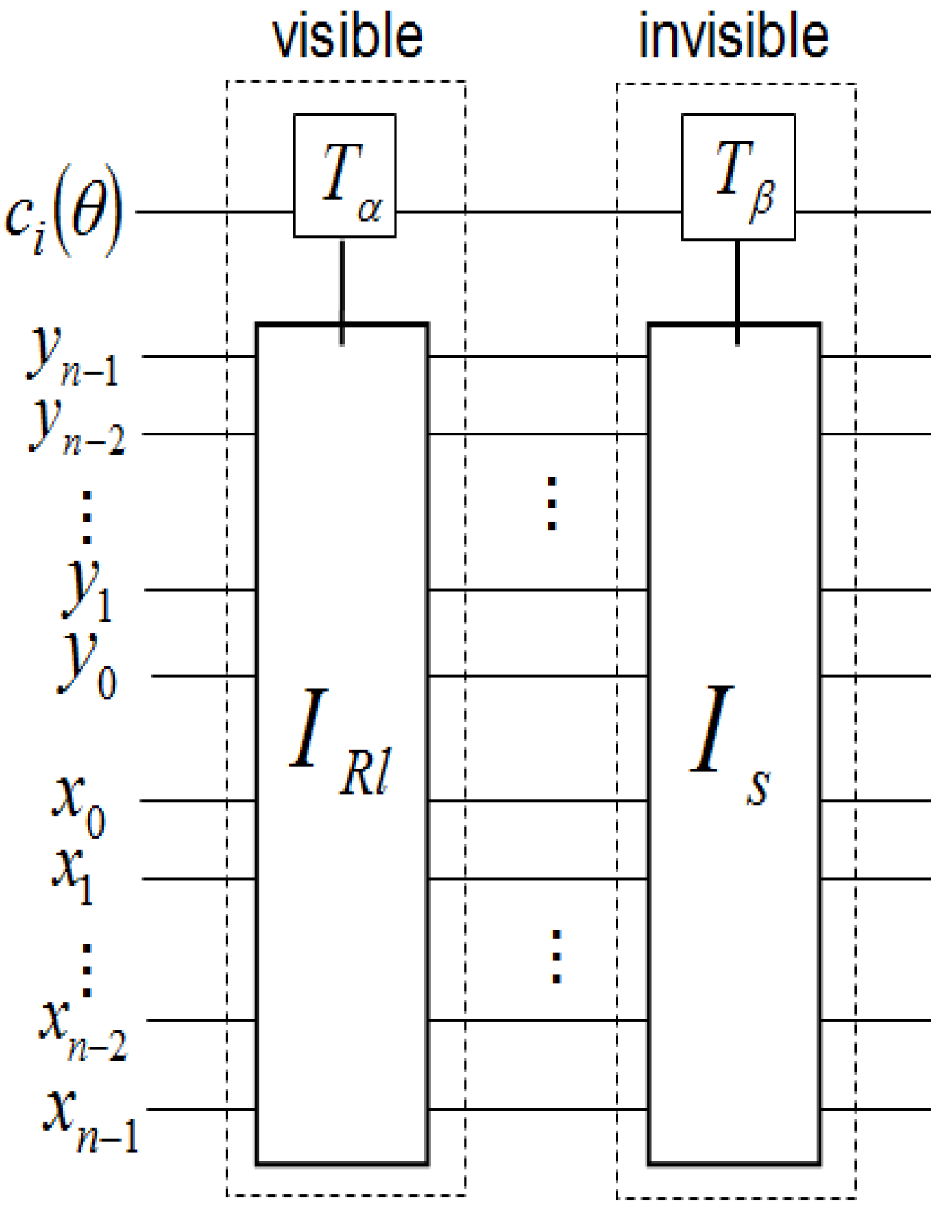
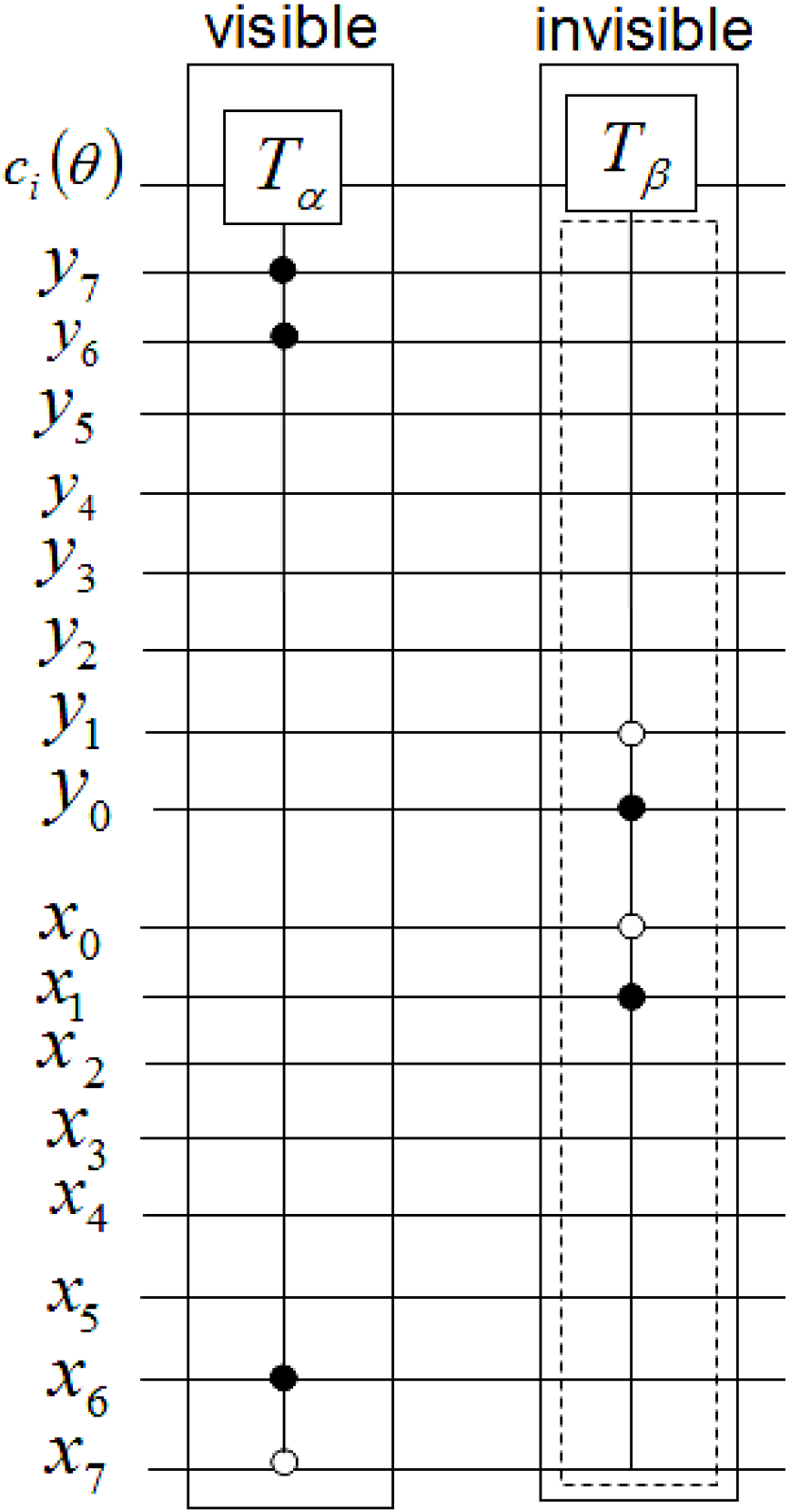
In this section, we introduce a modified or crude version of the standard ancilla-driven quantum computation (ADQC), which was highlighted earlier in this section, as the cornerstone of the proposed movie reader. Our proposed dependent ancilla-driven movie reader exploits the properties of single-qubit projective measurements and the entanglement-based interaction between the ancilla qubit and the register qubit of the ADQC. The measurements are performed dependent upon satisfying some predefined conditions based on the position of each point in the image, hence, the name dependent ancilla-driven movie reader. An elegant review of the projective measurements can be found in [74]. Here, we just recall, therefrom, a few notations that are indispensable to discussing our proposed movie reader.

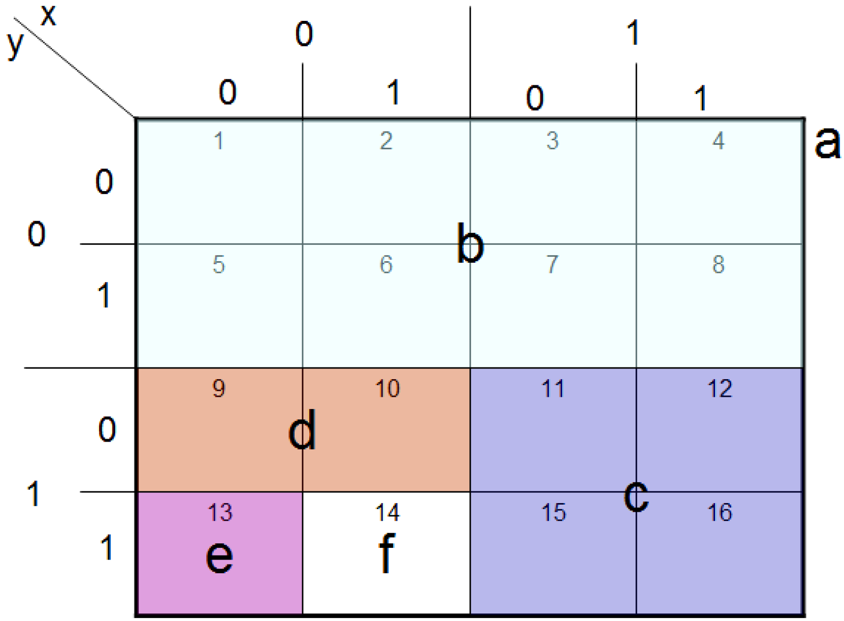
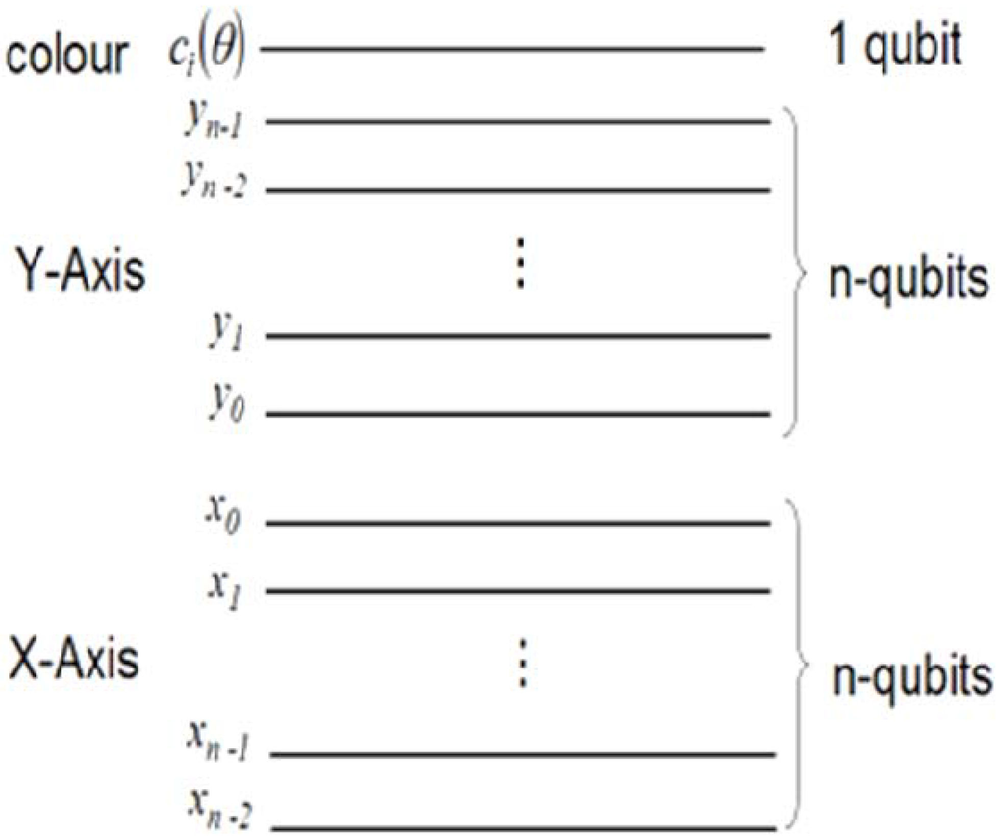
A projective measurement can be specified by orthogonal subspaces of the measured Hilbert space; the measurement projects the state onto one subspace and outputs (the readout) the subspace label. A single-qubit measurement along the computational basis $\left\{|0\rangle ,\hspace{0.17em}|1\rangle \right\}$ is equivalent to Mz and it returns a classical value that is the same as the label of that basis, in this case (0, 1). 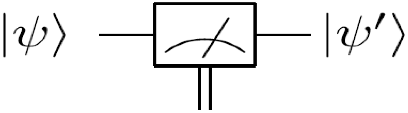We will adopt the notations and nomenclature from [75] for the measurement circuitry of our proposed movie reader. Throughout the rest of this review, a double line coming out of a measurement box represents a classical outcome, and a single line out of the same box represents the post-measurement quantum state being measured as exemplified in Figure 55 (and some of the circuits earlier in this section). Such a measurement is described by a set of operators Mr acting on the state of the system. The probability p of a measurement result r occurring when state ψ is measured is $\langle \psi |M_r^{\text{†}}{M}_r|\psi \rangle$. The state of the system after measurement $|{\psi }^{\prime }\rangle$is:

$$|{\psi }^{\prime }\rangle =\frac{M_r}{p_r}|\psi \rangle$$

(57)

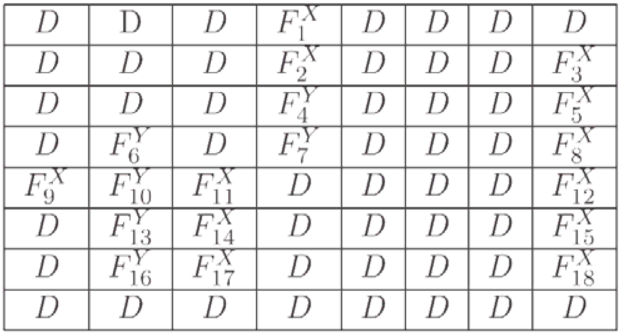
Figure 55. A single qubit measurement gate.

Figure 55. A single qubit measurement gate.

In the ADQC, the ancilla A is prepared and then entangled to a register qubit (in our case the single qubit encoding the colour information) using a fixed entanglement operator E. A universal interaction between the ancilla and register is accomplished using the controlled-Z (CZ) gate and a swap (S) gate and then measured. An ADQC with such an interaction allows the implementation of any computation or universal state preparation [36]. This is then followed by single qubit corrections on both the ancilla and register qubits.

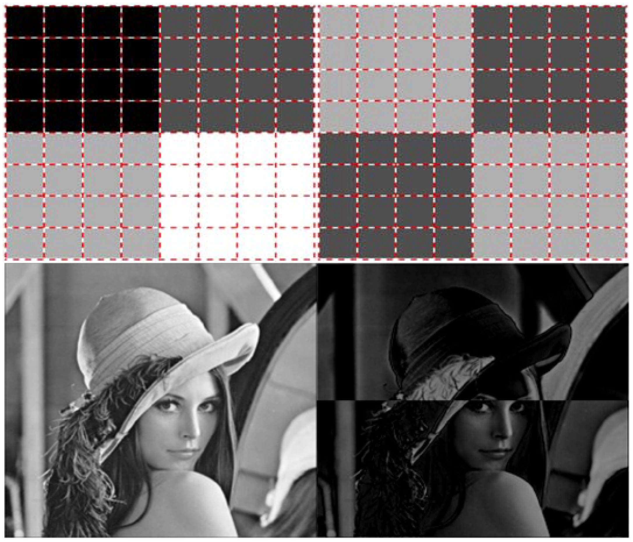
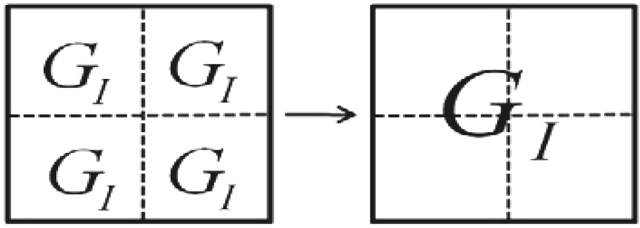
Figure 56. Exploiting the position information |i〉 of the FRQI representation to predetermined the 2D grid location of each pixel in a transformed image G_I(|I(θ)〉).

Figure 56. Exploiting the position information |i〉 of the FRQI representation to predetermined the 2D grid location of each pixel in a transformed image G_I(|I(θ)〉).

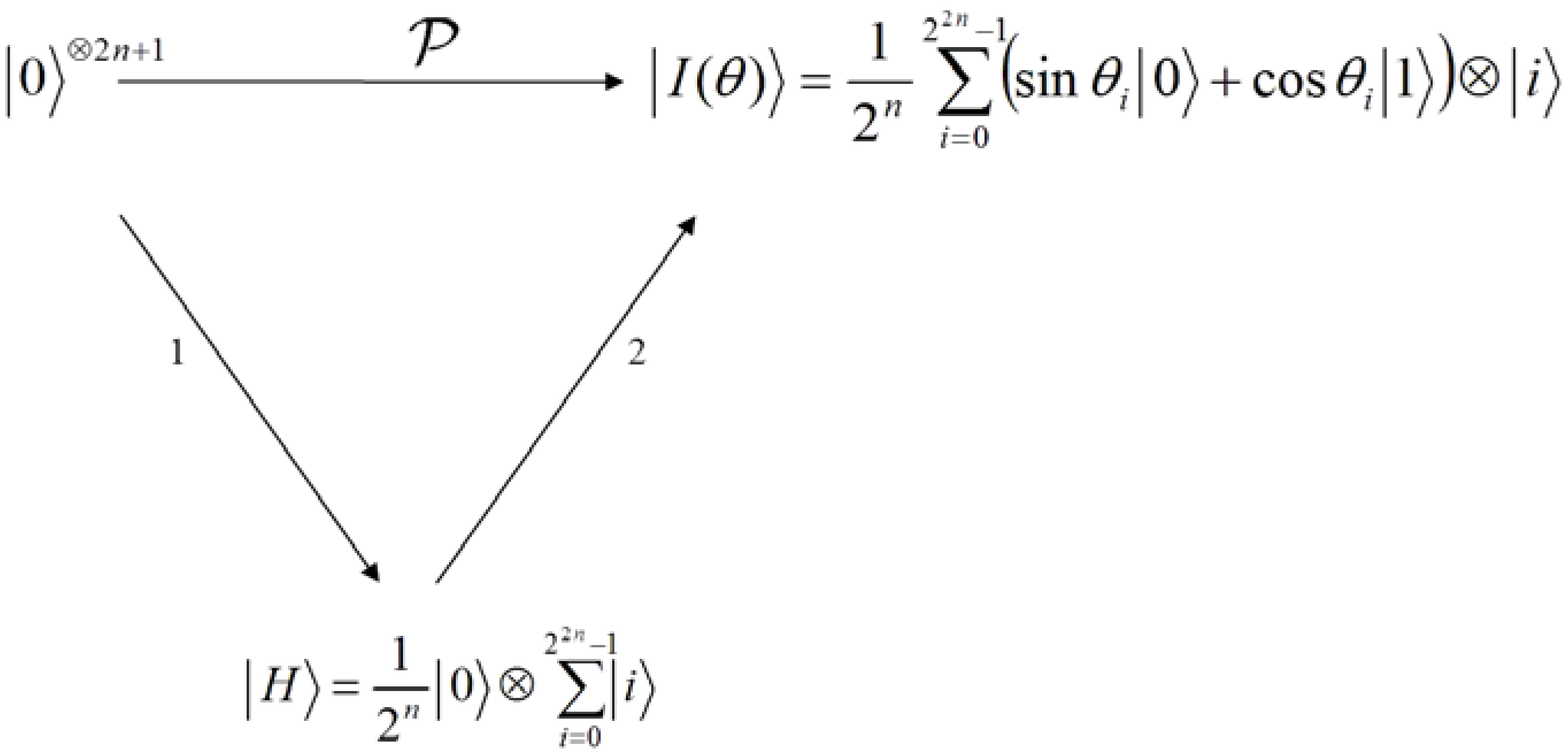
Having introduced these basic rudiments about the projective and ADQC measurements, we are equipped to transfer certain features of each of them to our proposed dependent ancilla-driven movie reader. In so doing, we exploit the fact that the position information about each pixel in an FRQI quantum image after transformation is known beforehand as discussed in earlier sections of this review, and presented in Figure 56. In other words, we have foreknowledge about the position where each pixel in an FRQI quantum image resides before and after being transformed. This vital knowledge reduces the amount of information required to recover the transformed image to just the information pertaining to the new colour of the pixels. We adopt the under listed simplifications for the purpose of recovering the colour of the $i^{th}$ pixel, $c_i$.

An interplay is assumed between the quantum CD and the movie reader. This enables the transfer of the ancillary information about the fill of every pixel as stored in the quantum CD to the reader as discussed earlier. Therefore, we simplify the representation for the ancilla states $|+\rangle$ and $|-\rangle$ from [38] as follows:

$$|+\rangle =|0\rangle ,\hspace{0.17em}\hspace{0.17em}\hspace{0.17em}\hspace{0.17em}\hspace{0.17em}\hspace{0.17em}\hspace{0.17em}\hspace{0.17em}\hspace{0.17em}|-\rangle =|1\rangle$$

(58)

for the absence and presence of a fill in that pixel, respectively:

• A universal interaction between the ancilla $|a\rangle$ and register (specifically, the colour qubit) is accomplished using the CZ gate and a swap (S) gate and then measured. An ADQC with such an interaction is sufficient for the implementation of any computation or universal state preparation [38].
• This is then followed by single qubit corrections, $Z^{\text{†}}$ and U on the ancillary information and colour of the pixel, respectively. The measurement to recover the colour of the $i^{th}$ pixel $M_i^{\theta }$ returns a value c_i as defined in Equation (2). Actually, this is the same as retaining the interaction operation E in the ADQC while replacing the measurement and Pauli corrections with a projective measurement as explained in [19].
• Finally, adopting the 2D grid position information of every point in a transformed key frame (FRQI state) shown in Figure 56 allows us to determine beforehand the required control-operations needed to recover the transformed key frame, i.e. the viewing frames. These conditions are summarised in Figure 57.

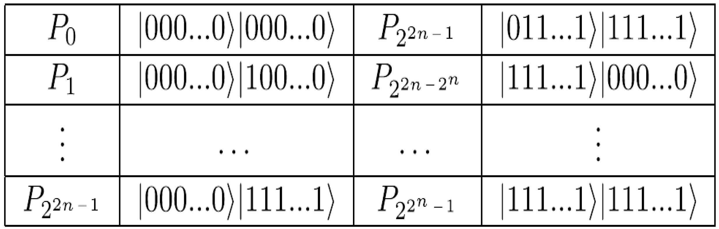
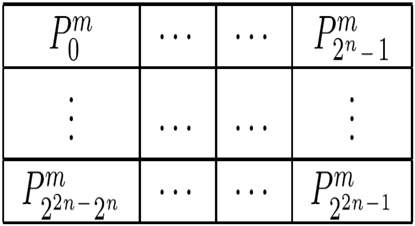
Figure 57. Control-conditions to recover the readout of the pixels of a 2ⁿ×2ⁿ FRQI quantum image.

Figure 57. Control-conditions to recover the readout of the pixels of a 2ⁿ×2ⁿ FRQI quantum image.

Exploiting this characteristic, a 2ⁿ×2ⁿ FRQI image can be recovered by tracking the changes it undergoes as dictated by movie script using the various elements of the movie circuit. The position information of each pixel as summarised in Figure 57 serves as the dependency on which the measurement to recover the colour information of each pixel is based. This implies that, each measurement recovers the colour of a specific pixel as specified by this position-specific information. In addition, the measurement is driven by the ancillary information about the colour (specifically, the fill of each pixel) as stored in the quantum CD.

Figure 58. Predetermined recovery of the position information of an FRQI quantum image. The * between the colour |c(θ_i)〉 and ancilla |a〉 qubits indicates the dependent ancilla-driven measurement as described in Figure 59 and Theorem 4.

Figure 58. Predetermined recovery of the position information of an FRQI quantum image. The * between the colour |c(θ_i)〉 and ancilla |a〉 qubits indicates the dependent ancilla-driven measurement as described in Figure 59 and Theorem 4.

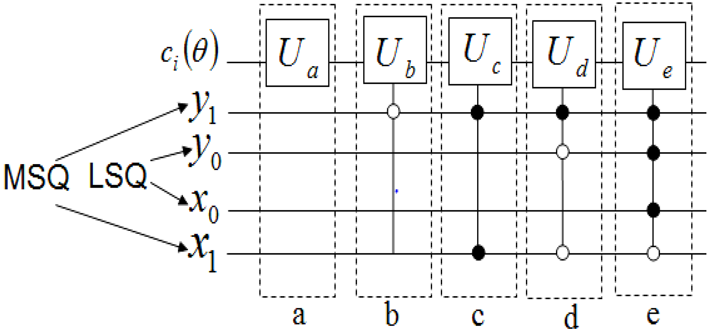
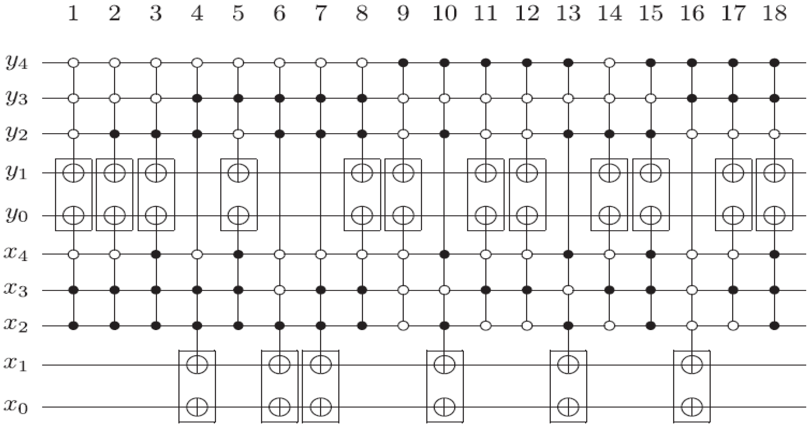
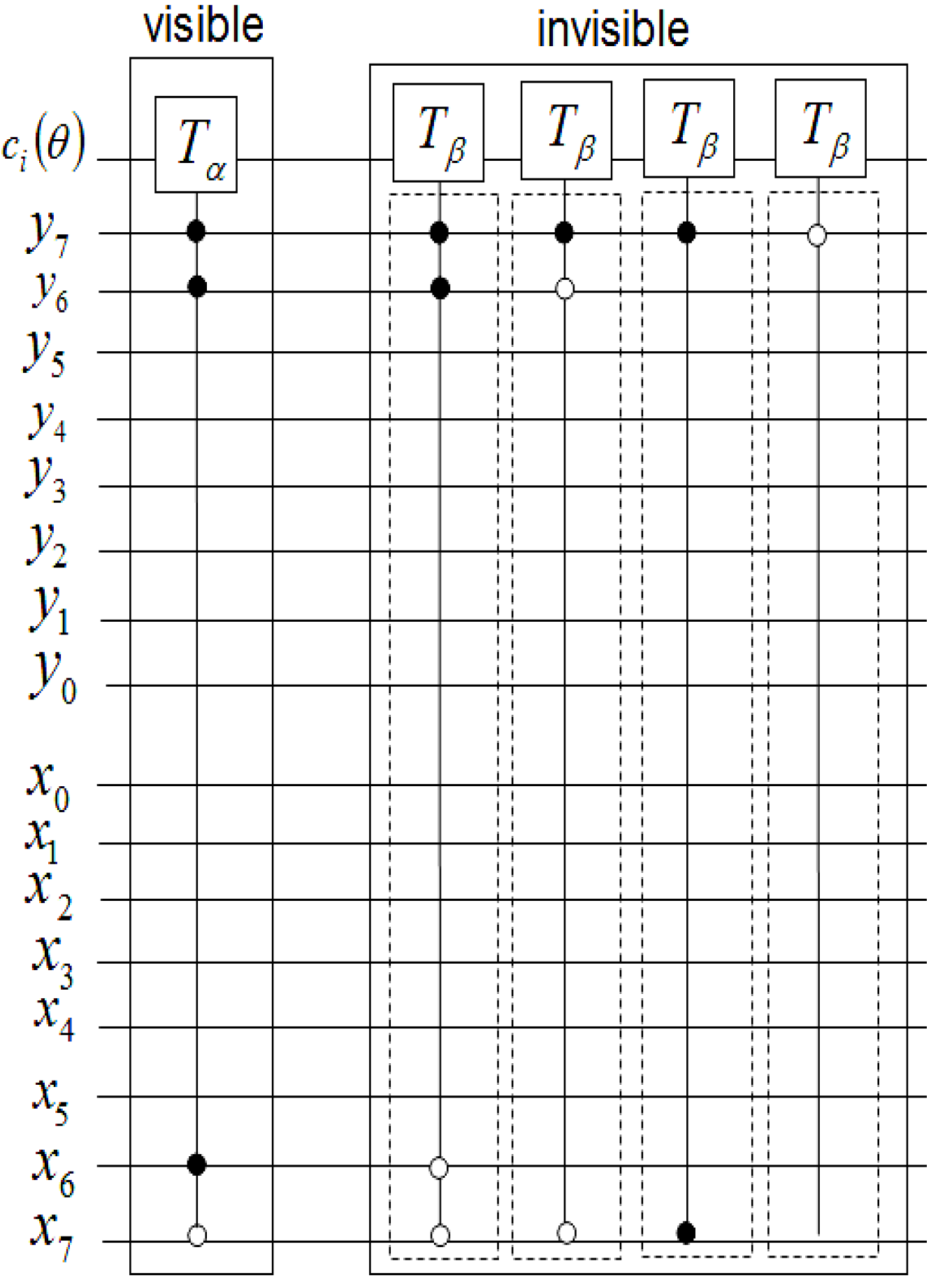
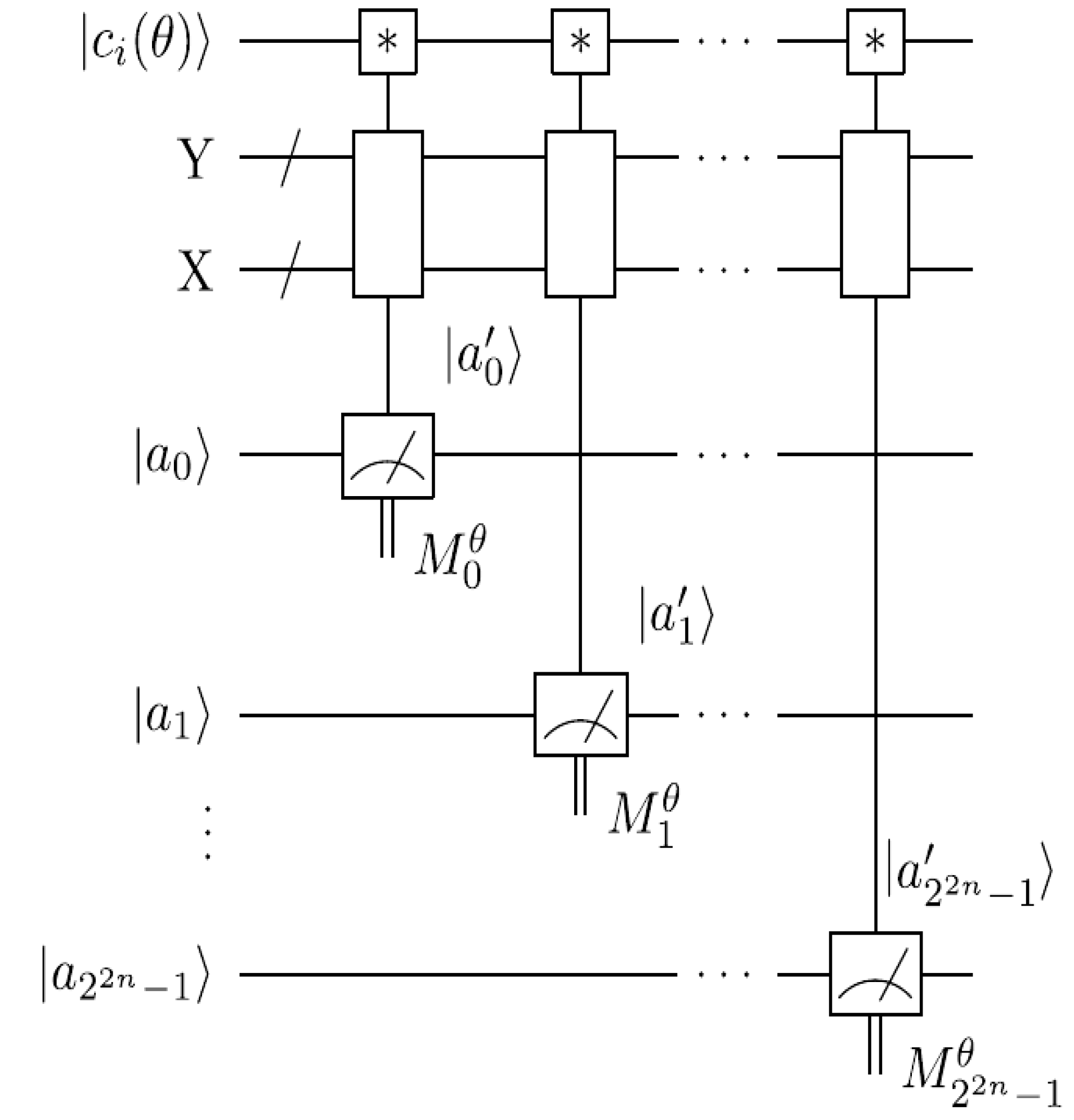
The measurements entail 2ⁿ × 2ⁿ dependent ancilla-driven measurement on each key (makeup or viewing) frame that makes the final movie sequence. The circuit in Figure 58 shows such a dependent ancilla-driven image reader. In this figure the rectangular boxes on the position information indicate the position dependency, which we will discuss at length in the sequel. In this format each measurement $M_i^{\theta }$ connecting the colour and ancilla qubits is of the form shown in Figure 59.

Theorem 4 (Image Reader Theorem) A total of $\hspace{0.17em}{2}^{2n}-1$ dependent ancilla-driven measurements $\hspace{0.17em}{M}_i$ of the colour $\hspace{0.17em}|c\left({\theta }_i\right)\rangle$ each as defined in Figure 59 are sufficient to recover the readout of the $i^{th}$ pixel of a 2n×2n FRQI quantum image where $i\in \left\{\hspace{0.17em}0,\hspace{0.17em}1,\hspace{0.17em}\cdots ,\hspace{0.17em}{2}^{2n}-1\right\}$.

Proof: We assume the dependency criteria of the image reader as indicated by the rectangular boxes in Figure 58 have been satisfied. Therefore, each measurement $M_i$ on pixel $p_i$ is performed only once for each readout. In addition to this, ignoring the post-measurement sign of the ancilla qubit, we adopt the elegant proof for similar circuits in [6] for our proof using Figure 59. Our objective is to show that the input state $|{\psi }_{in}\rangle$ and the initial state of the ancilla qubit $|a\rangle$ are unaltered by the transformations that yield measurement $M_i$, while the classical readout of $|{\psi }_{in}\rangle$ is recovered:

$$|{\psi }_{in}\rangle =|c\left({\theta }_i\right)\rangle ,\hspace{0.17em}\hspace{0.17em}\hspace{0.17em}\hspace{0.17em}\hspace{0.17em}\hspace{0.17em}\hspace{0.17em}\hspace{0.17em}\hspace{0.17em}|a\rangle =|c\left({\theta }_i\right),\hspace{0.17em}a\rangle ,\hspace{0.17em}\hspace{0.17em}\hspace{0.17em}\hspace{0.17em}\hspace{0.17em}\hspace{0.17em}\hspace{0.17em}|{\psi }_1\rangle =|\overline{c}\left({\theta }_i\right),\hspace{0.17em}a\rangle$$

(59)

where $|\overline{a}\rangle =Z|a\rangle$. Similarly:

$$|\overline{c}\left({\theta }_i\right)\rangle =Z|c\left({\theta }_i\right)\rangle ,\hspace{0.17em}\hspace{0.17em}\hspace{0.17em}\hspace{0.17em}\hspace{0.17em}\hspace{0.17em}\hspace{0.17em}\hspace{0.17em}\hspace{0.17em}|{\psi }_2\rangle =|\hspace{0.17em}a,\hspace{0.17em}\left(c\left({\theta }_i\right)\oplus a\right)\oplus a\rangle ,\hspace{0.17em}$$

$$\hspace{0.17em}|{\psi }_2\rangle =|\hspace{0.17em}a,\hspace{0.17em}\overline{c}\left({\theta }_i\right)\rangle ,\hspace{0.17em}\hspace{0.17em}\hspace{0.17em}\hspace{0.17em}\hspace{0.17em}\hspace{0.17em}\hspace{0.17em}\hspace{0.17em}\hspace{0.17em}\hspace{0.17em}\hspace{0.17em}|{\psi }_3\rangle =|\hspace{0.17em}a,\hspace{0.17em}{\overline{c}}^{\prime }\left({\theta }_i\right)\rangle ,$$

where $|c^{\prime }\left({\theta }_i\right)\rangle$ is the post-measurement state of $|c\left({\theta }_i\right)\rangle$ as defined in Equation (58):

$$\hspace{0.17em}|{\psi }_4\rangle =|\hspace{0.17em}\hspace{0.17em}{\overline{c}}^{\prime }\left({\theta }_i\right),\hspace{0.17em}a\rangle ,\hspace{0.17em}\hspace{0.17em}\hspace{0.17em}\hspace{0.17em}\hspace{0.17em}\hspace{0.17em}\hspace{0.17em}\hspace{0.17em}\hspace{0.17em}\hspace{0.17em}\hspace{0.17em}|{\psi }_{out}\rangle =|\hspace{0.17em}\hspace{0.17em}{\overline{\overline{c}}}^{\prime }\left({\theta }_i\right),\hspace{0.17em}a\rangle .$$

Since:

$$\hspace{0.17em}Z|\hspace{0.17em}\hspace{0.17em}\overline{c^{\prime }}\left({\theta }_i\right)\rangle =|\hspace{0.17em}\hspace{0.17em}{\overline{\overline{c}}}^{\prime }\left({\theta }_i\right)\rangle =|\hspace{0.17em}\hspace{0.17em}{c}^{\prime }\left({\theta }_i\right)\rangle ,$$

we therefore conclude that:

$$|{\psi }_{out}\rangle =|\hspace{0.17em}\hspace{0.17em}{c}^{\prime }\left({\theta }_i\right),\hspace{0.17em}a\rangle .$$

(60)

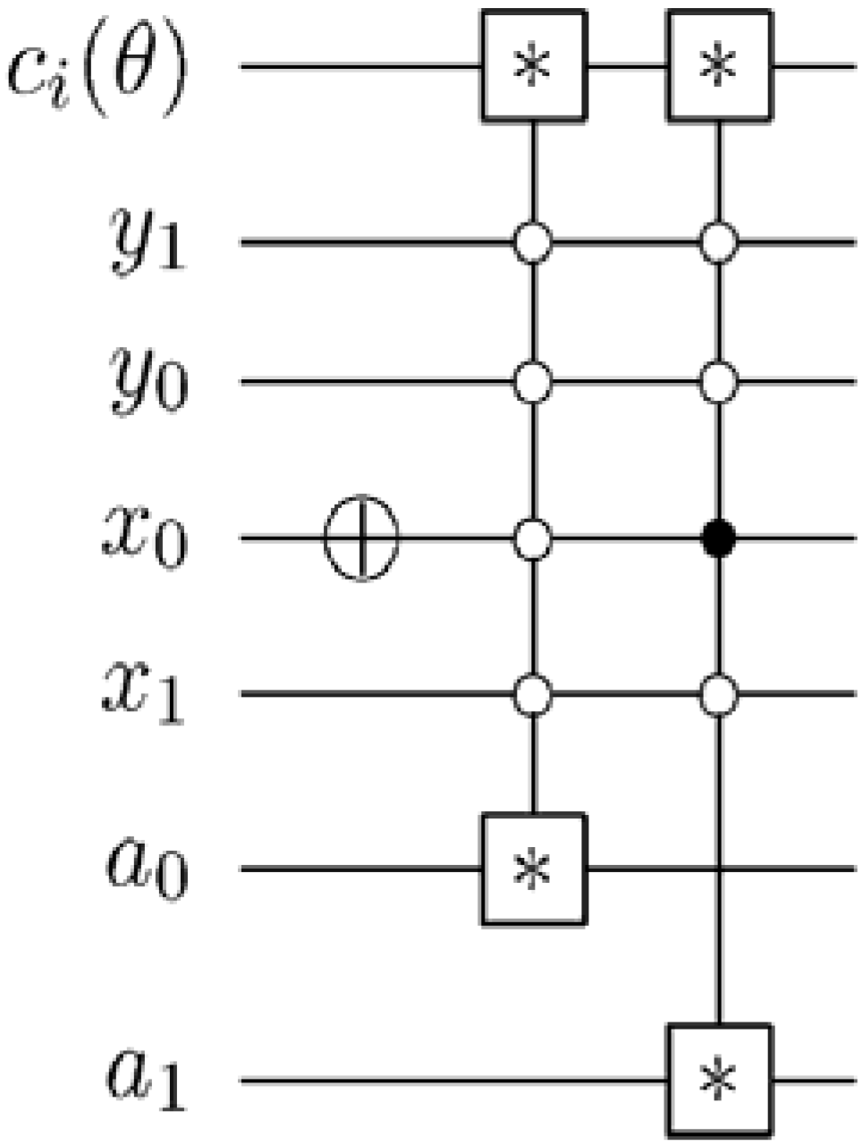
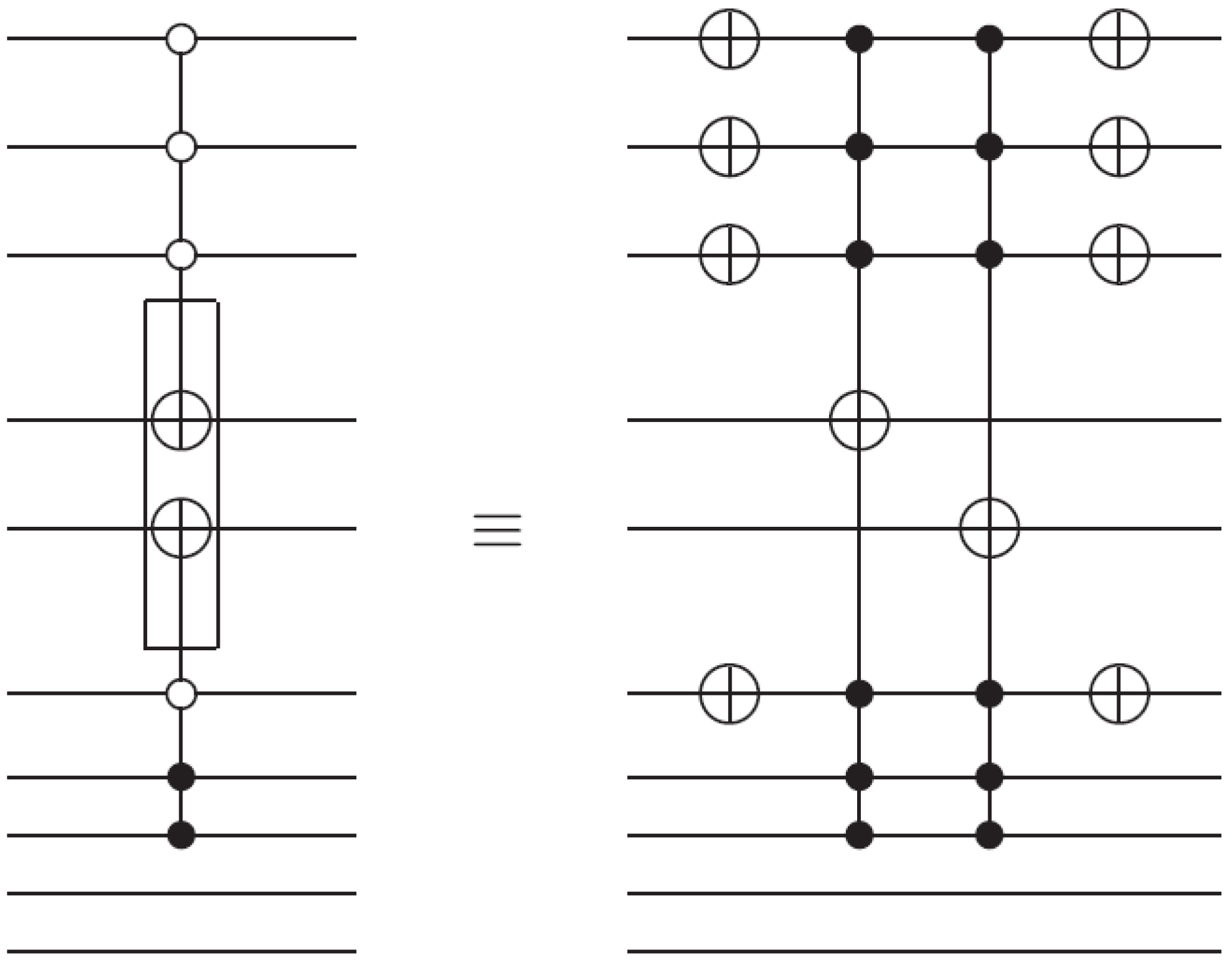
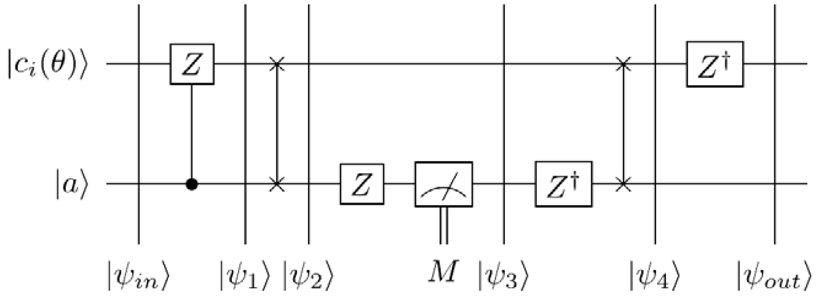
Figure 59. Circuit to recover the content of the single-qubit colour information of an FRQI quantum image. This circuit represents each of the * between the colour and ancilla qubit in Figure 58.

Figure 59. Circuit to recover the content of the single-qubit colour information of an FRQI quantum image. This circuit represents each of the * between the colour and ancilla qubit in Figure 58.

Simple inspection of our output state $|{\psi }_{out}\rangle$ in Equation (60) proves that for a pixel whose ancilla qubit $|a\rangle =|1\rangle ,\hspace{0.17em}\hspace{0.17em}\hspace{0.17em}\hspace{0.17em}\hspace{0.17em}|{\psi }_{out}\rangle =|c\left({\theta }_i\right),\hspace{0.17em}a\rangle$ because using Equation (57) and [73] $|c^{\prime }\left({\theta }_i\right),\hspace{0.17em}a\rangle =|c\left({\theta }_i\right)\rangle$. Similarly, from our explanation of the ancillary information earlier in this section, it is obvious that for a pixel whose ancilla information $|a\rangle =|0\rangle$, the colour angle ${\theta }_i=0$ and hence $|c\left({\theta }_i\right)\rangle$ as defined in Equation (2) becomes $|c\left({\theta }_i\right)\rangle =0$. Therefore, $|c^{\prime }\left({\theta }_i\right),\hspace{0.17em}a\rangle =|c\left({\theta }_i\right)\rangle$.

Hence, we conclude that the post-measurement state of our readout:

$$|{\psi }_{out}\rangle =|\hspace{0.17em}\hspace{0.17em}c\left({\theta }_i\right),\hspace{0.17em}a\rangle$$

(61)

And therefore:

$$|{\psi }_{in}\rangle =|\hspace{0.17em}{\psi }_{out}\rangle$$

Our proposed dependent ancilla-driven measurements in Figure 58 and Figure 59, and Theorem 3 combines features from the projective and ADQC measurement techniques as reviewed in the earlier parts of this section. As seen in Figure 58 and the explanation that emanated from it, the measurements are performed depending on whether or not some predetermined conditions are satisfied. These conditions are necessary in order to confine the measurement $M_i$ to pixel $p_i$.

Utilising our foreknowledge about the position of the pixels in an FRQI quantum image before and after its transformation, we could generalise the position dependency portrayed earlier by the rectangular boxes (on the position axis in Figure 58) to obtain the image reader circuit for a single FRQI quantum image (in our case a key, makeup, or viewing frame) as presented in Figure 60. These are additional constraints that must be satisfied before the ancillary measurement described in Figure 58 and Theorem 4 are carried out. Each pair of ∗ connecting the colour and ancilla qubits is a circuit of the form shown in Figure 59.

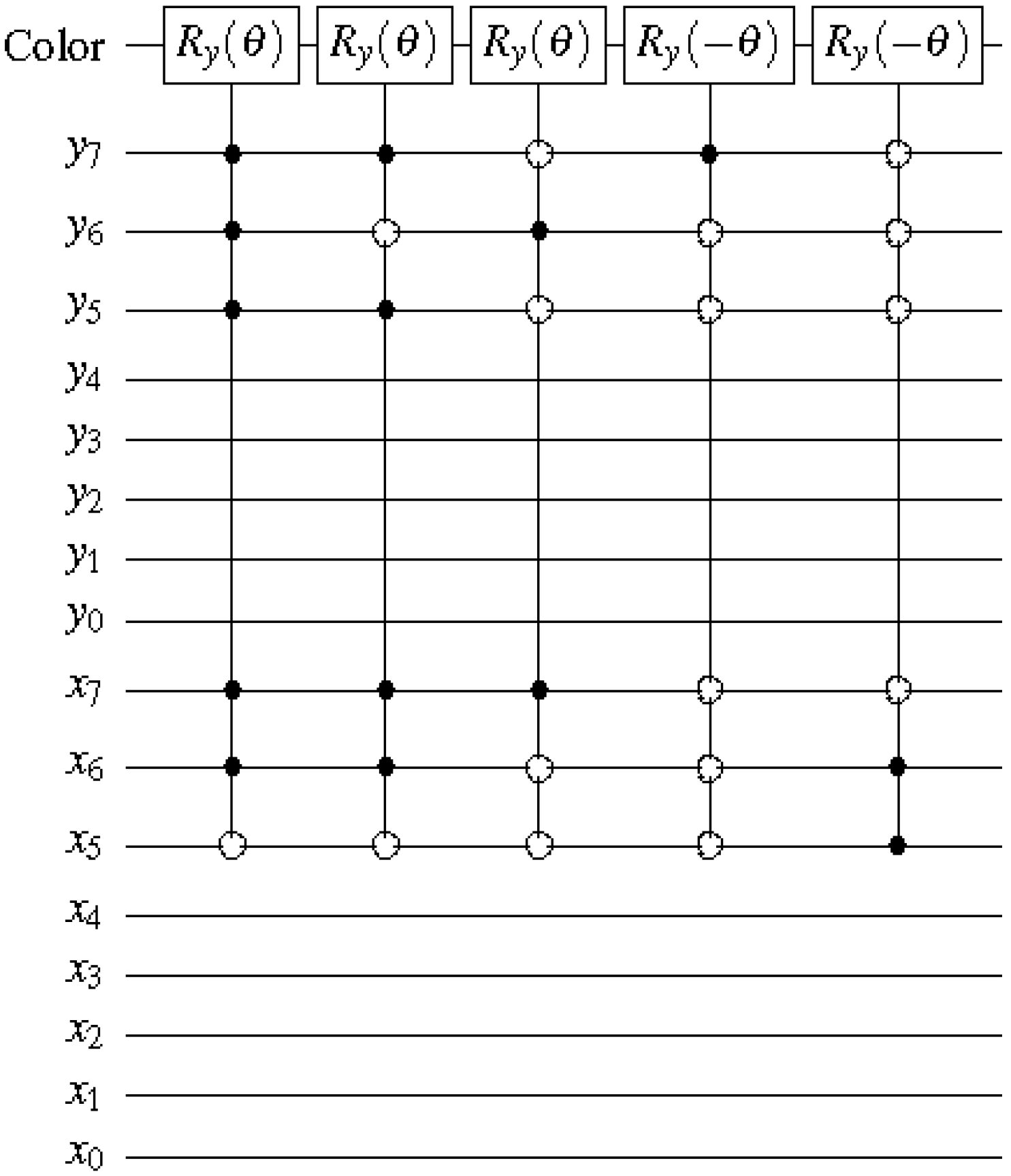
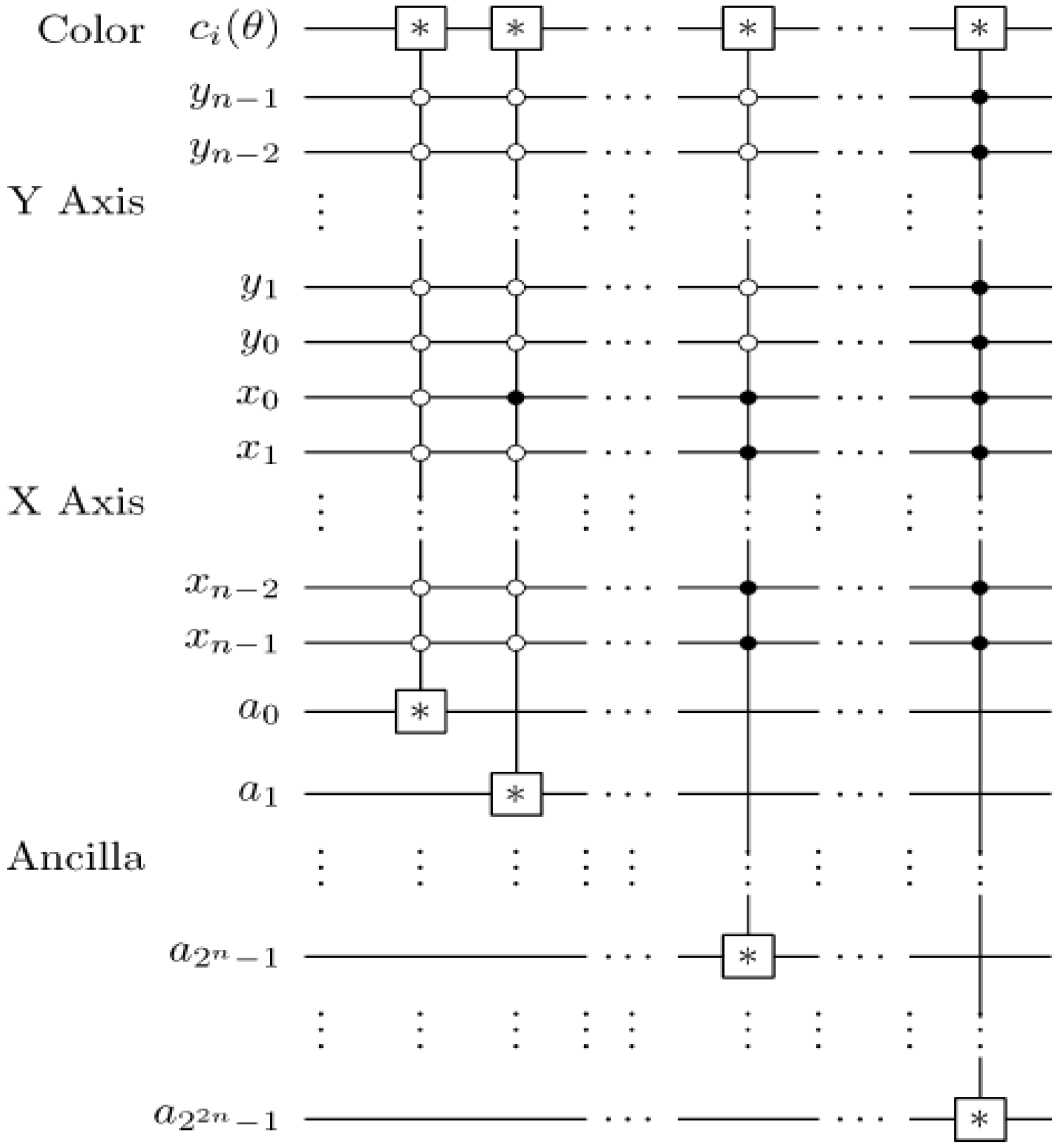
Figure 60. Reader to recover the content of a 2ⁿ×2ⁿ FRQI quantum image.

Figure 60. Reader to recover the content of a 2ⁿ×2ⁿ FRQI quantum image.

Using this format, the changes in the ancillary information (whether each pixel in the original image, a key frame, has a fill or not) undergoes can be tracked relative to changes in their colours as they evolve based on the transformations by the movie and CTQI operations.

In recovering the contents of a movie, however, multiple such measurements are necessary. Definition 6 formalises our definition of the movie reader.

Definition 6: An mFRQI quantum movie reader is a system comprising $2^{2n}-1$ ancillary qubits each initialised as defined earlier in this section and Equation (58) to track the change in the content of every pixel in each frame (key, makeup, or viewing) that forms part of the movie sequence in Equation (56) based on single-qubit dependent ancilla-driven measurements as described in Figure 60.

As proposed in this section, any destructive measurement on our movie reader like in the ADQC is made on the ancilla [38,75], while the key (makeup and viewing) frame content remains intact for future operations. It is a method for implementing any quantum channel on a quantum register driven by operations on an ancilla using only a fixed entangling operation. Using the ADQC, measurements on each of the frames in the movie sequence $|M\rangle$ in Equation (58) produce its classical version resulting in a sequence called the viewing sequence, M given as

$$\begin{array}{l}M=F_0\left(f_{0,0},f_{0,1},\hspace{0.17em}\cdots ,\hspace{0.17em}{f}_{0,p}\right)\hspace{0.17em}{K}_1^0{F}_1,\hspace{0.17em}\cdots ,\hspace{0.17em}{F}_2^{m-1}\\ \hspace{0.17em}\hspace{0.17em}\hspace{0.17em}\hspace{0.17em}\hspace{0.17em}\hspace{0.17em}\hspace{0.17em}\hspace{0.17em}\hspace{0.17em}\hspace{0.17em}\hspace{0.17em}\hspace{0.17em}\hspace{0.17em}\times \left(f_{2^m-1,0},\hspace{0.17em}{f}_{2^m-1,1},\hspace{0.17em}\cdots ,f_{2^m-1m-1,q}\right)\hspace{0.17em}{F}^{2^m}.\end{array}$$

(62)

At appropriate frame transition rates (classically, 25 frames per second [65]), its sequence creates the impression of continuity in the movements of the frame content as dictated by the script of the movie.

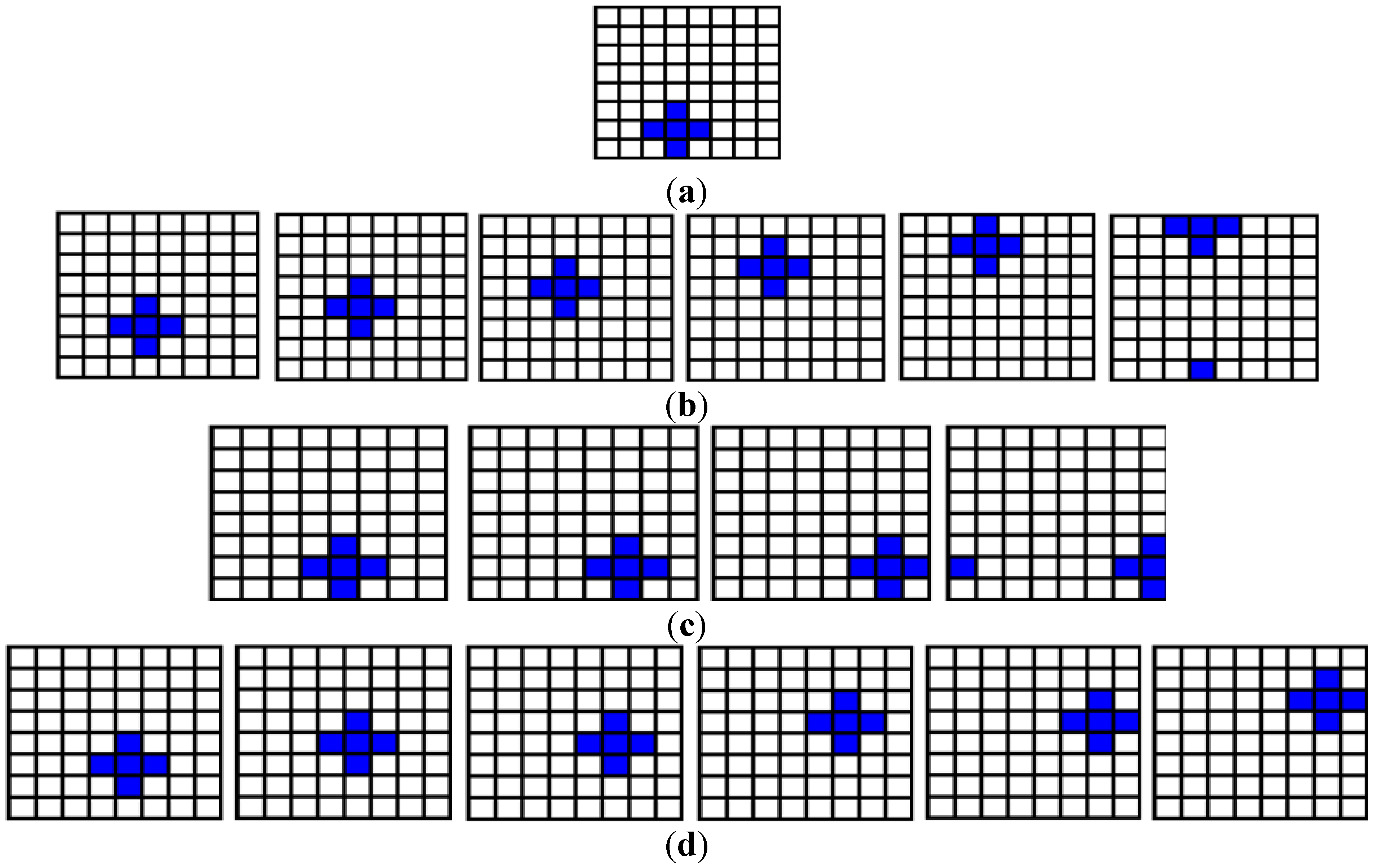
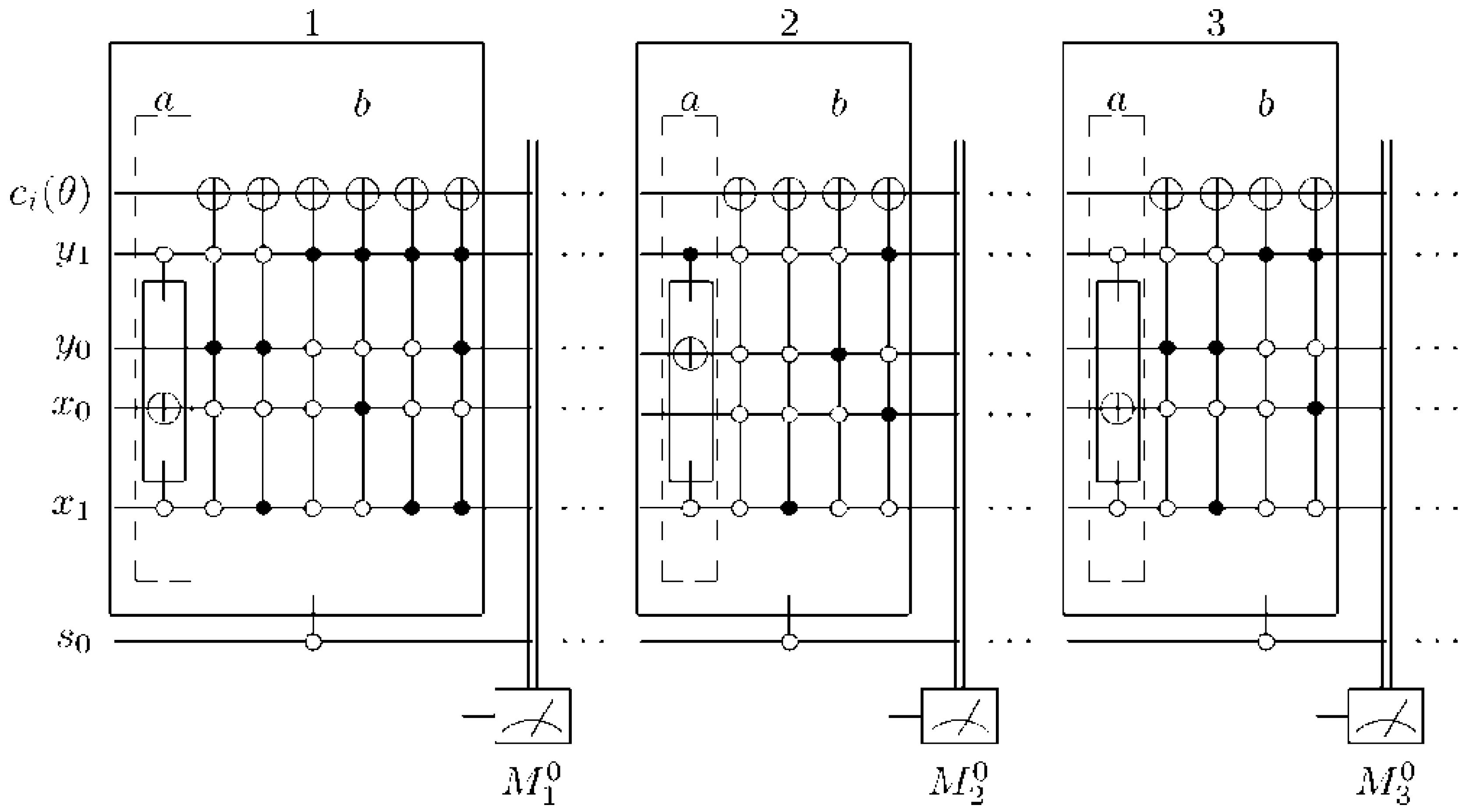
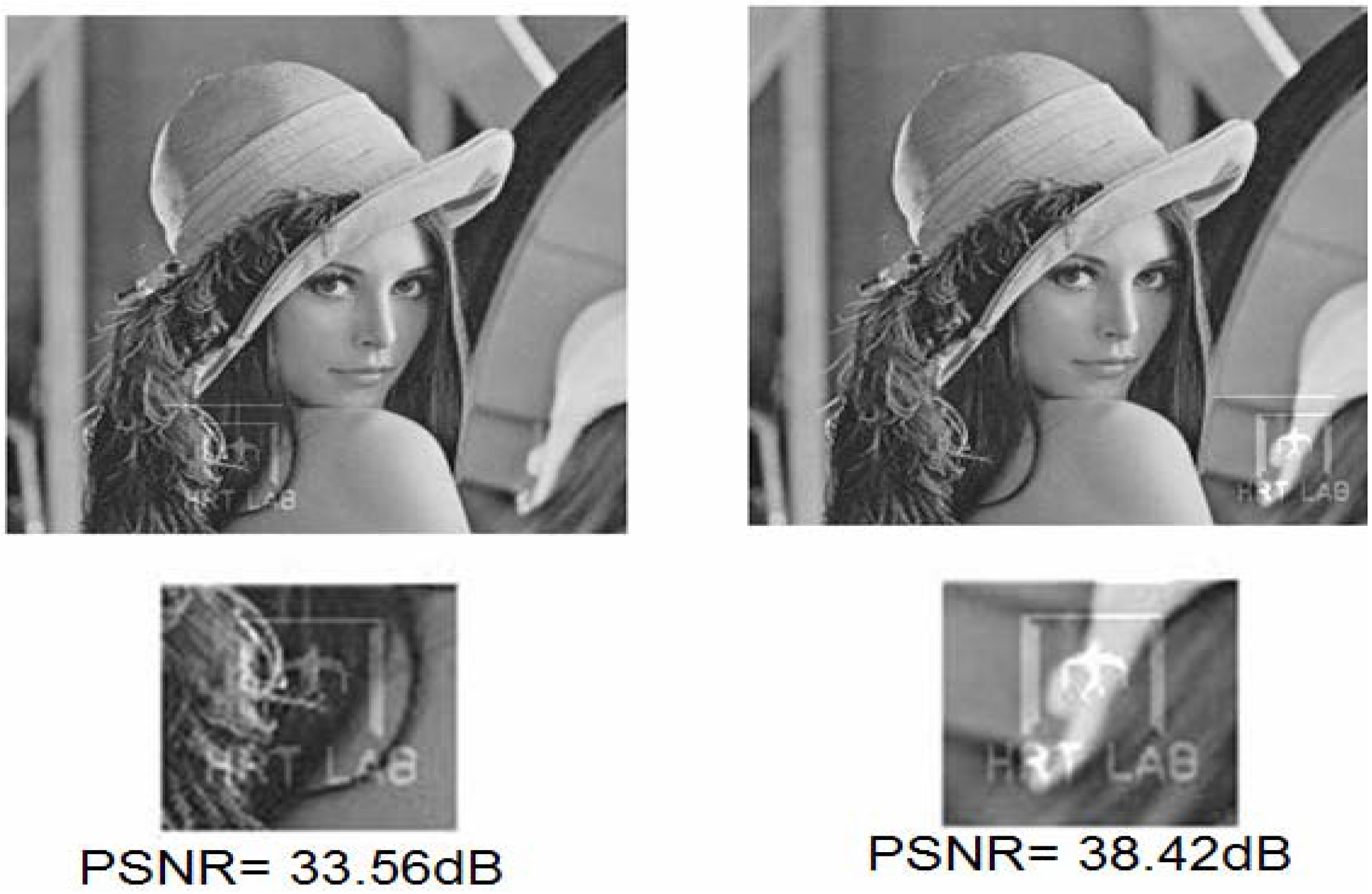
To conclude, we consider the use of our dependent ancilla-driven movie reader to recover the movie sequence for the scene presented in Figure 49 and discussed earlier in this section. Based on the key frame for this example as presented in Figure 49(d), the ancillary information consists of 16 ancilla qubits which are prepared as $|a_0\rangle$ through $|a_{15}\rangle$. This information as stored in the quantum CD comprises: the first qubit $|a_0=1\rangle$, while all the others are prepared in state $|0\rangle$ as explained in [19] and earlier parts of this section. The movie reader performs a total of $16\times \left(1+3\right)$ measurements each of the form described in Figure 60 in order to obtain the final classical readout of the movie sequence of this scene.

For brevity, we limit the recovery of movie sequence by the movie reader to just the first viewing frame $|f_{0,1}\rangle$. The movie reader readout as read by the measurement layer $M_0$ indicates the new states of the 16 pixels from their original states in the key frame $|F_0\rangle$ to those in $|f_{0,1}\rangle$ as transformed by the SMO and CTQI operations in sub-circuit 1 of Figure 50 in the form described in Figure 56. As explained in subsection 6.2, this sub-circuit comprises two parts labelled (a) and (b) for the SMO and CTQI operations, respectively.

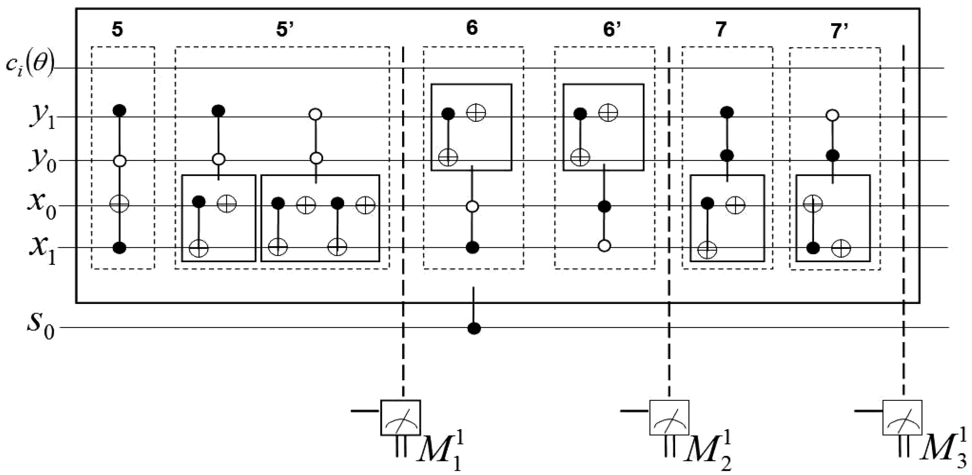
The purpose of measurement $M_0$ (which is itself a sub-part of the movie reader) is to track the evolution of the key frame $|F_0\rangle$ as it undergoes various transformations, which are in turn dictated by the movie script. For clarity, we further divide the measurement $M_0$ of the movie circuit in Figure 50 into three groups. The first two groups each focus on new states (of the pixels) obtained by transforming the colour and (or) position content of $|F_0\rangle$. The third group focuses on the pixels of $|F_0\rangle$ that were not transformed by the movie circuit, i.e. pixels that the script requires unchanged between the transitions (evolution) of the content from $|F_0\rangle$ to $|f_{0,1}\rangle$. These three groups are discussed in the sequel.

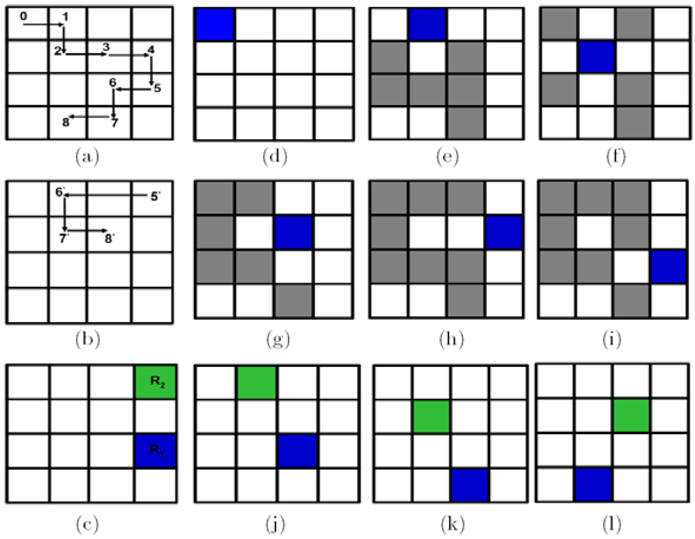
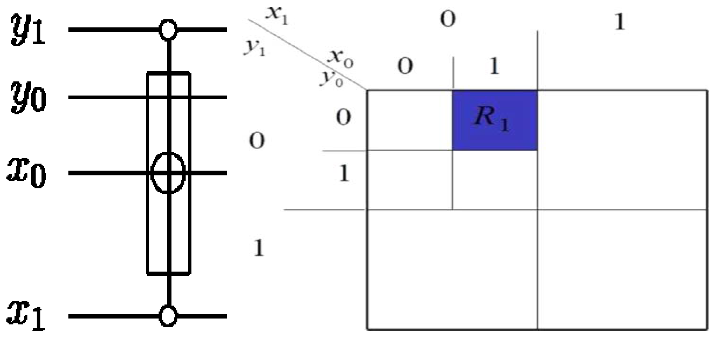
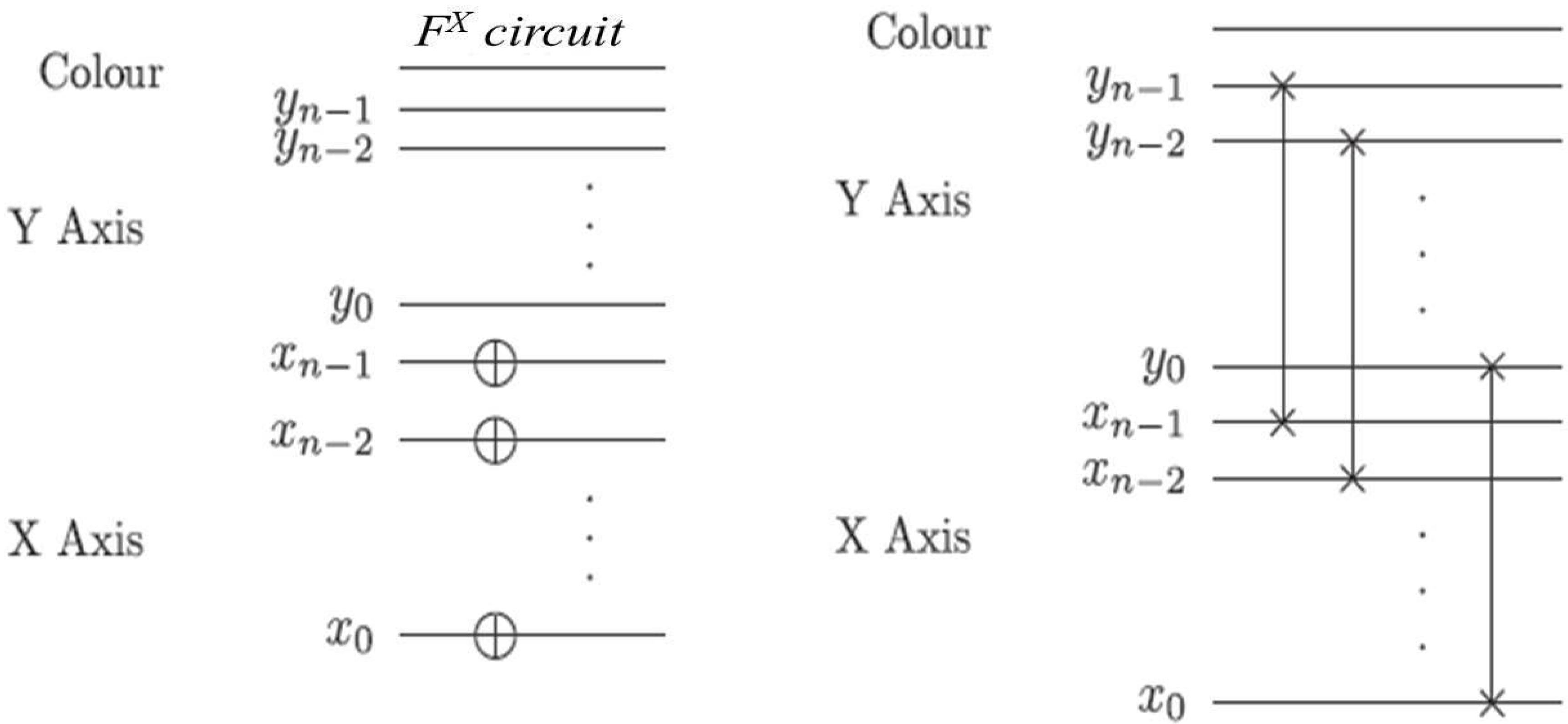
As specified by the movie script, our ROI at pixel $p_0$ (in $|F_0\rangle$) moves one step forward which is realised by using the $M_F^c$ operation as shown in sub-circuit 1(a) of Figure 50. The effect is a swap in the contents of pixels $p_0$ and $p_1$. Hence, no CTQI operation is involved in this transformation. To recover the new content of these pixels, we must track the transformations in their respective positions.

Tracking the transformations in their respective positions becomes simplified by considering the colour and position information of each pixel as an entangled state [2,8] as discussed earlier in section. In this regard, the new readouts 0 and 1 in $|f_{0,1}\rangle$ for pixel $p_0$ and $p_1$, respectively, are easily visualised. A transformation that changes the position of either or both of these pixels transforms both their colour and position together. The movie reader sub-circuit to recover these two pixels is presented in Figure 61.

The second group considers pixels for which the effect of the sub-circuit 1 manifests only in changes in the colour content of the key frame. By studying sub-circuit 1, specifically, sub-circuit 1(b), we realise that there are six such pixels namely $p_4$, $p_6$, $p_8$, $p_9$, $p_{10}$ and $p_{14}$. The position-dependency information of each of these pixels (Figure 56) is used to track the colour transformations on these pixels. The movie reader sub-circuit in Figure 62 shows the interaction between the movie reader (specifically, the measurement $M_0$) and the quantum player, which facilitates the readout of the new contents of the pixels as transformed by sub-circuit 1(b). For brevity, we have used a single X gate on $|c\left({\theta }_i\right)\rangle$ to show the transformation of the contents of all the six pixels (in actual sense, each pixel is transformed separately by such an operation). This (use of a single qubit) is possible because the pixels have the same colour both before ($|0\rangle$, i.e. with $\theta =\frac{\pi }{2}$ and hence, all their ancilla’s are in state $|0\rangle$) and after the transformations in the frames F0 and $|f_{0,1}\rangle$, respectively. The operation on the colour qubit transforms the colour from state $|0\rangle$ to $|1\rangle$. Meanwhile, the ∗ connecting the colour and ancilla qubit facilitates the recovery of the new states subject to satisfying the position-dependency on $|y_{n-1}{y}_{n-2}\cdots y_0\rangle |x_{n-1}{x}_{n-2}\cdots x_0\rangle$. 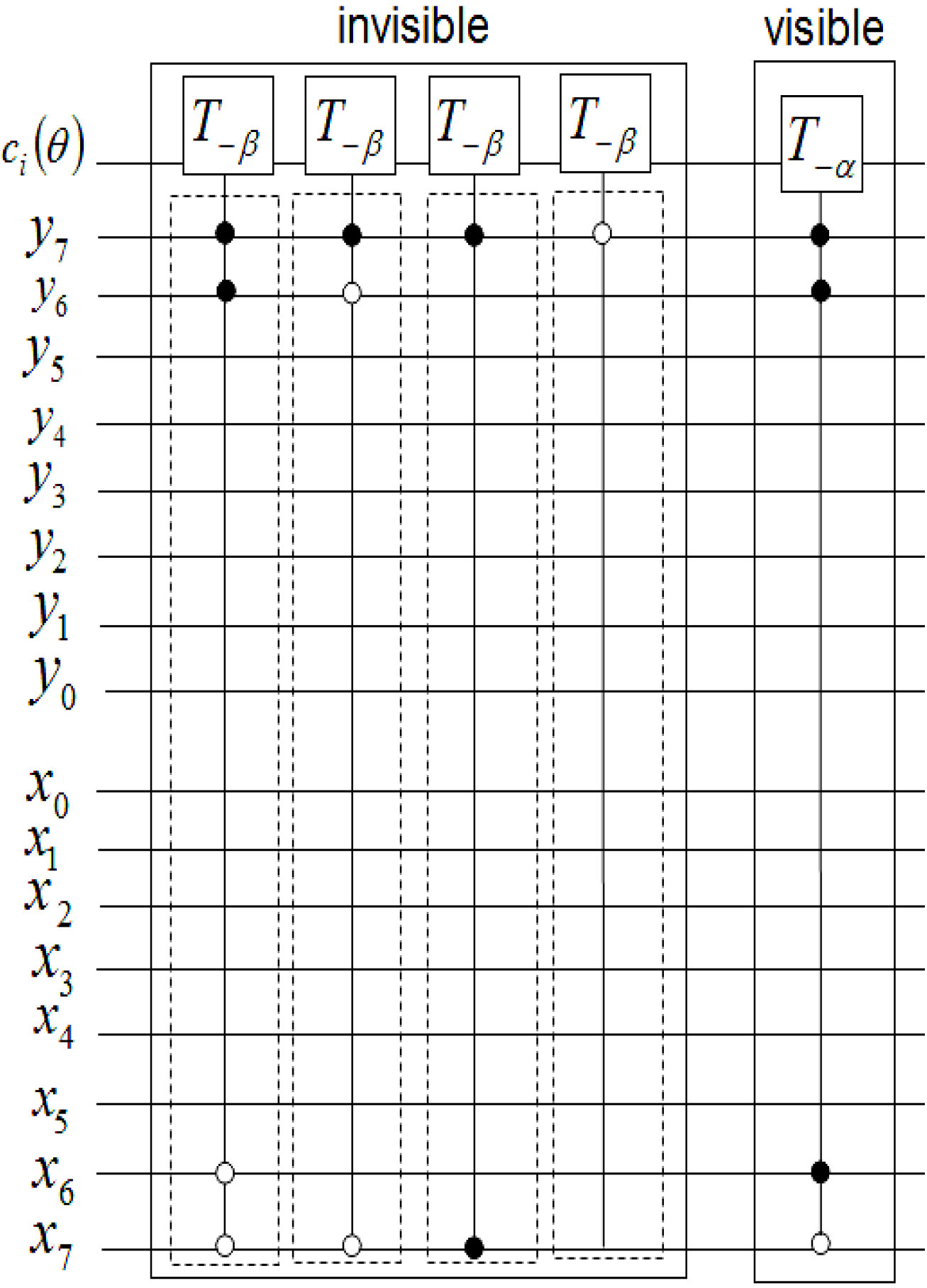The circuit in Figure 63 demonstrates how such readout is obtained for pixel $p_4$ while the same procedure suffices to recover the content of the remaining five pixels.

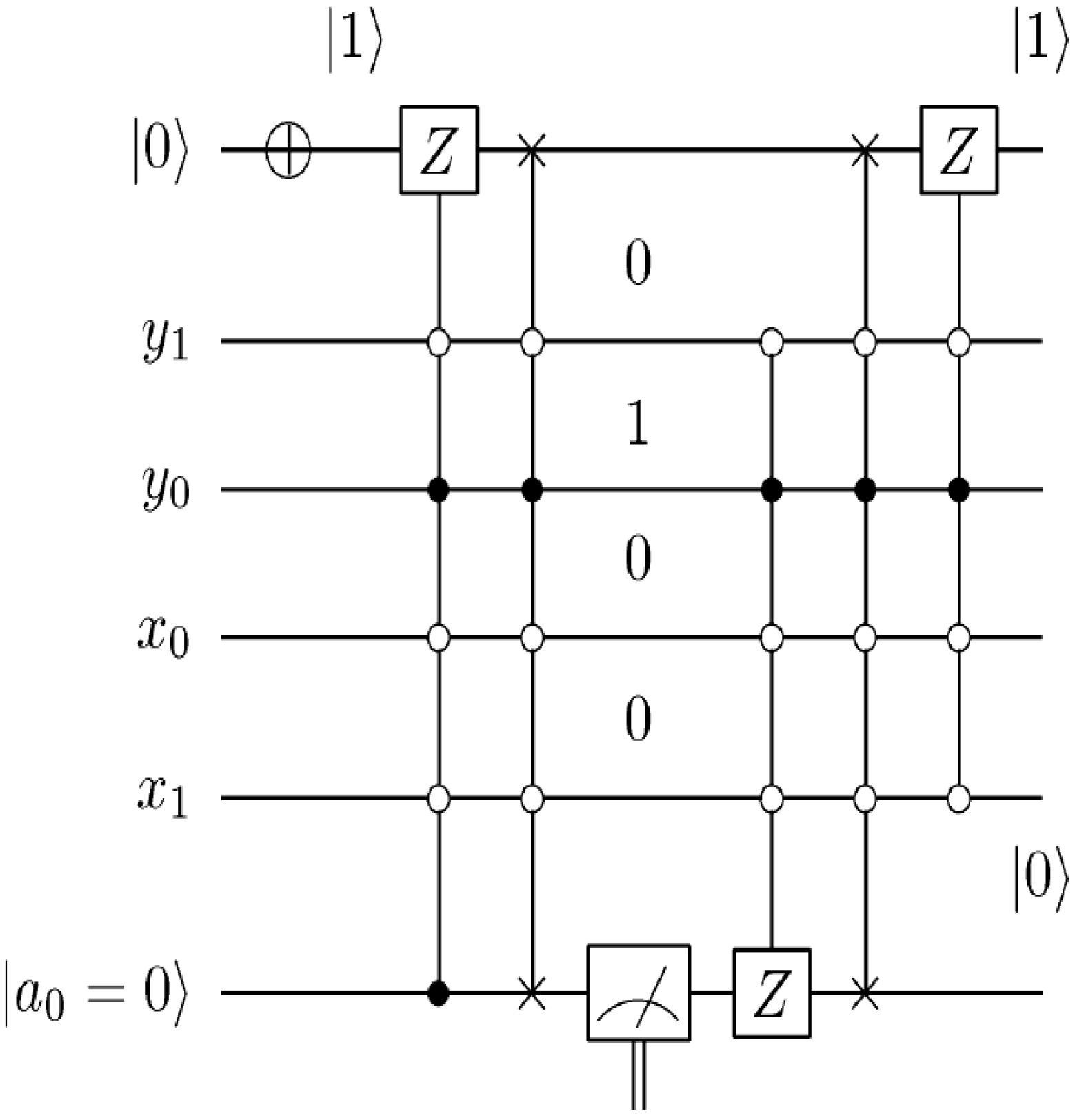
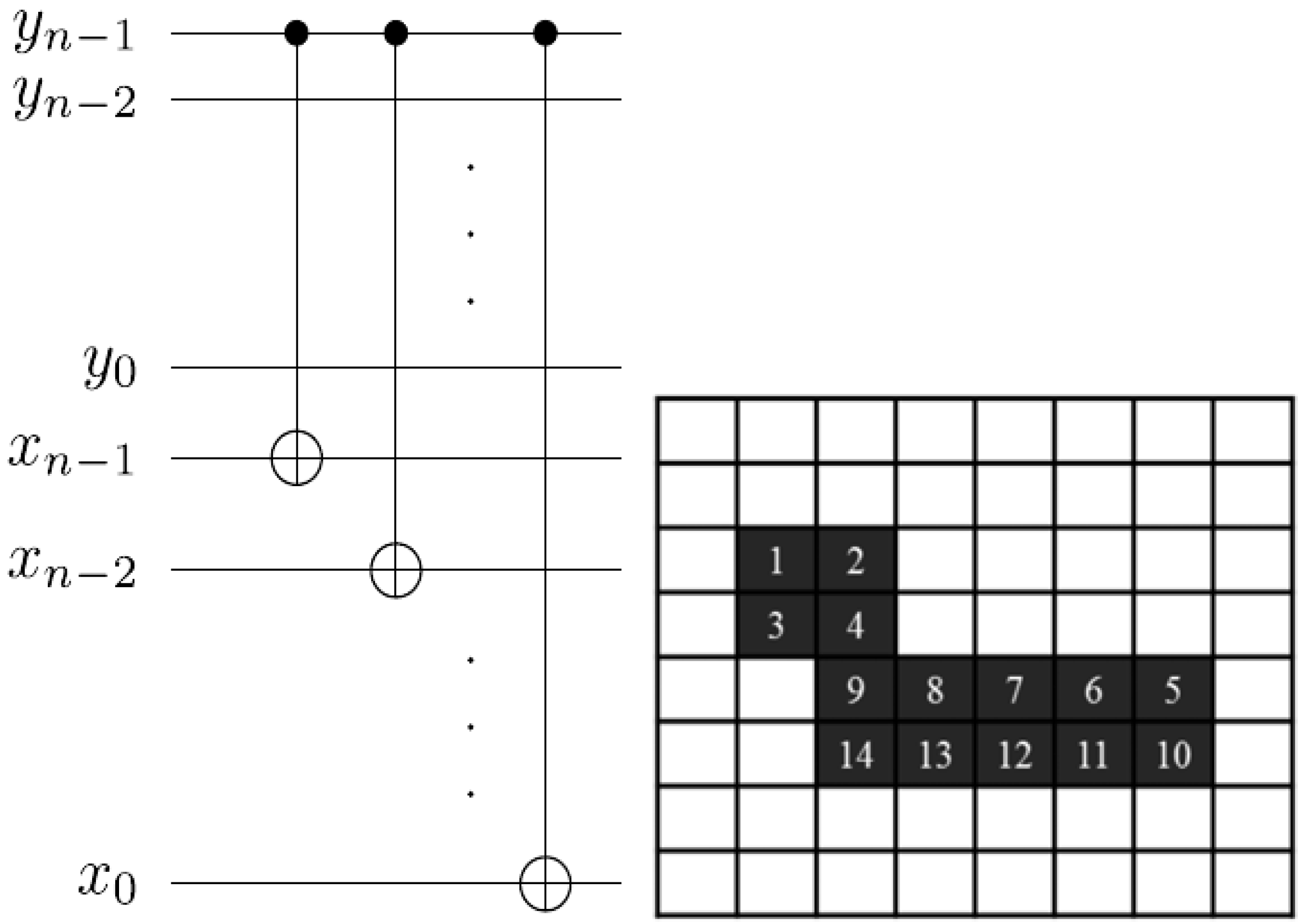
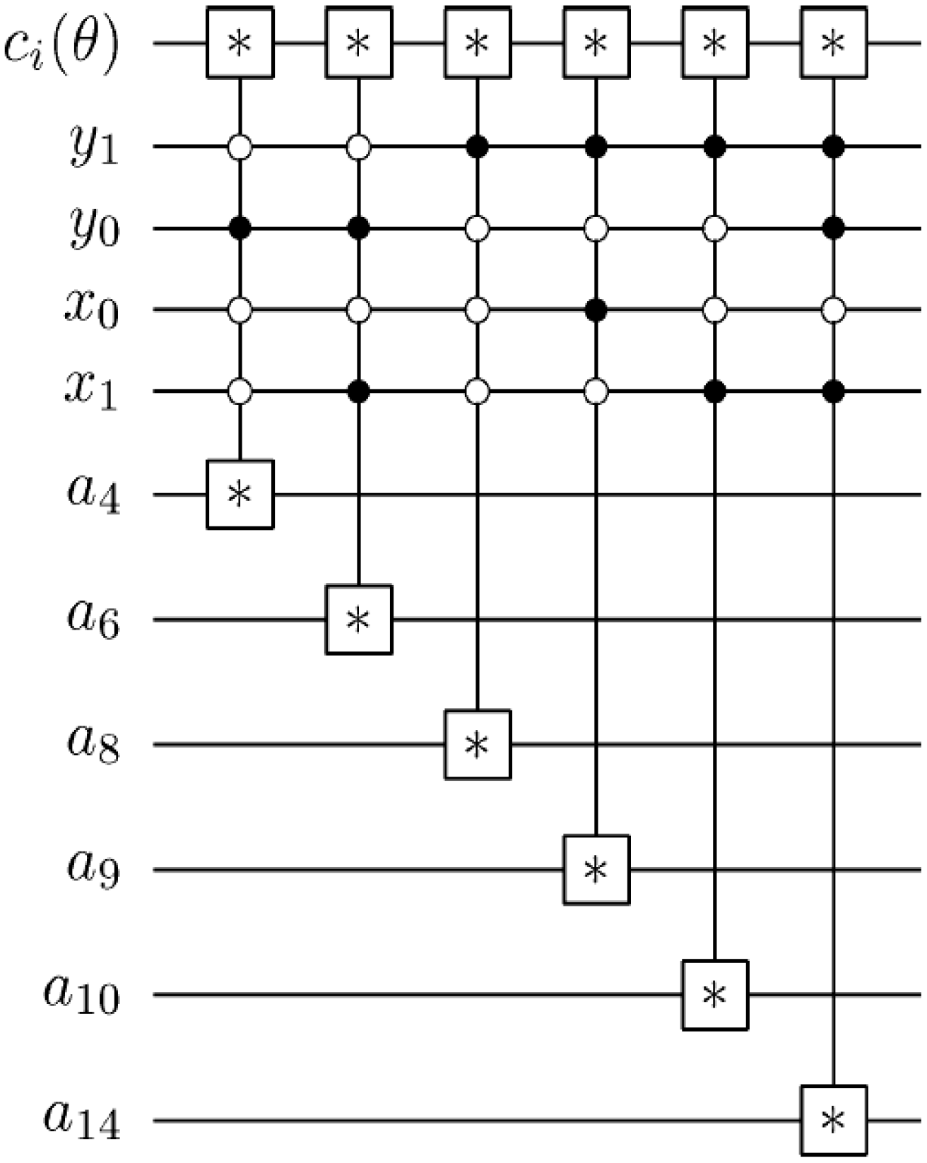
Figure 61. Movie reader sub-circuit to recover pixel p₀ and p₁ for frame |f_0,1〉 corresponding to Figure 49e.

Figure 61. Movie reader sub-circuit to recover pixel p₀ and p₁ for frame |f_0,1〉 corresponding to Figure 49e.

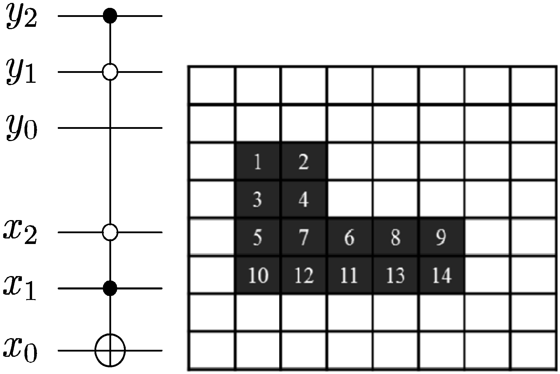
Figure 62. Movie reader to recover pixels p₄, p₆, p₈, p₉, p₁₀ of viewing frame |f_0,1〉.

Figure 62. Movie reader to recover pixels p₄, p₆, p₈, p₉, p₁₀ of viewing frame |f_0,1〉.

Figure 63. Readout of the new state of pixel p₄ as transformed by sub-circuit 1 in Figure 52.

Figure 63. Readout of the new state of pixel p₄ as transformed by sub-circuit 1 in Figure 52.

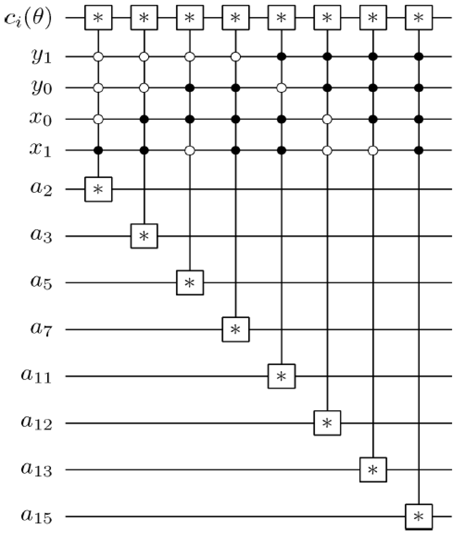
Figure 64. Movie reader sub-circuit to recover the content of pixels p₂, p₃, p₇, p₁₁, p₁₂, p₁₃ and p₁₅.

Figure 64. Movie reader sub-circuit to recover the content of pixels p₂, p₃, p₇, p₁₁, p₁₂, p₁₃ and p₁₅.

The last group consists of eight pixels whose colour and position information are not transformed by sub-circuit 1 of the movie circuit in Figure 50. Hence, the colour and position of these pixels are unchanged in $|F_0\rangle$ and $|f_{0,1}\rangle$. Combining the simplifications discussed earlier with the position-dependency information in Figure 56, we obtain a movie reader sub-circuit which is enough to track the changes in the content of these pixels. This sub-circuit is presented in Figure 64, where each ∗ connecting the colour and ancilla qubits is equivalent to the measurement circuit in Figure 59. All the eight pixels being measured in this group (using the sub-circuit 1 in Figure 50 and the measurement circuit in Figure 64) are characterised by ancillary and colour that are both in state $|0\rangle$, i.e. $|c\left({\theta }_i\right)=0\rangle$ and $|a\rangle =0$. As presented in Theorem 4, each ∗ connecting the colour and ancilla qubits produces readout 0, i.e. the label of the measurement on $|c\left({\theta }_i\right)=0\rangle$.

By combining the three movie reader sub-circuits, circuits from these groups, we obtain the larger movie reader sub-circuit to recover the viewing frame $|f_{0,1}\rangle$. Extending similar techniques to the measurements $M_1-M_8$ in the movie circuit in Figure 52, we can recover the content of each of the viewing frames in Figure 49(e)–(l) of the scene.

6.4. The Cat, the Mouse, and the Lonely Duck: A Quantum Movie

An example that utilises the various tools required to demonstrate the representation and production of quantum movies as it pertains to the operation of the quantum CD and player is presented in this section.

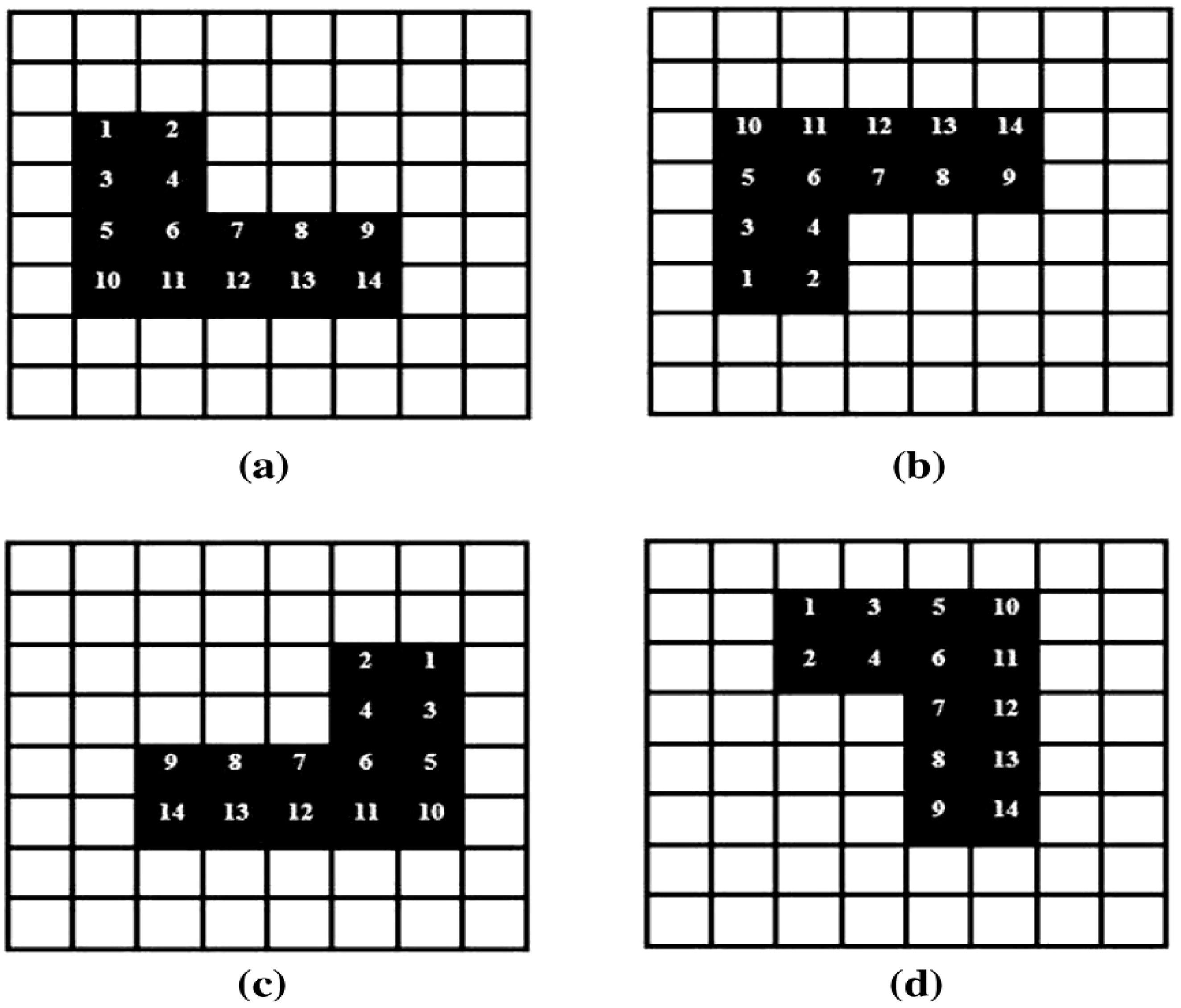
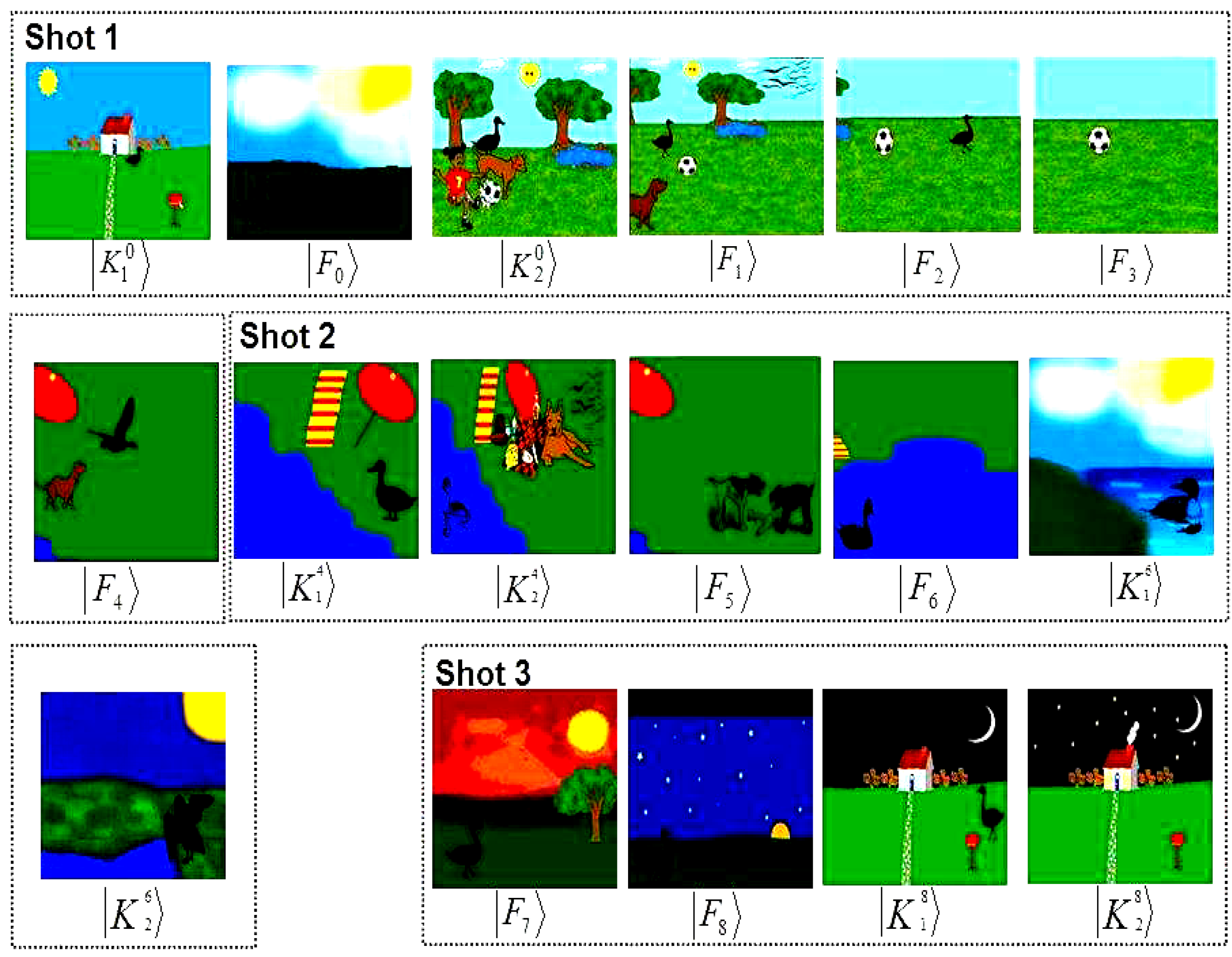
In this example, we assume that the director in liaison with the circuitor have carefully studied the script (usually in writing) and concluded that the key and makeup frames in Figure 65 and Figure 66 are adequate to effectively convey the two scenes of the movie which is entitled “The cat, the mouse, and the lonely duck”. The first scene entitled “The lonely duck goes swimming” consists of three shots of varying length and hence varying order and number of key and makeup frames. Similarly, the second scene is made up of 23 key and makeup frames which are divided into the two shots of the scene. Based on the content of this scene, it is appropriately entitled “The cat and mouse chase”.

The two scenes show how divergent contents of a movie can be conveyed using the operations discussed earlier in this section. The scenes involve varying content, movement, pace, and finally, the example illustrates how the frame-to-frame transition operation is used to cover the entire length of the 40-frame movie strip.

Figure 65. Key and makeup frames for the scene “The lonely duck goes swimming”. See text and [19] for additional explanation.

Figure 65. Key and makeup frames for the scene “The lonely duck goes swimming”. See text and [19] for additional explanation.

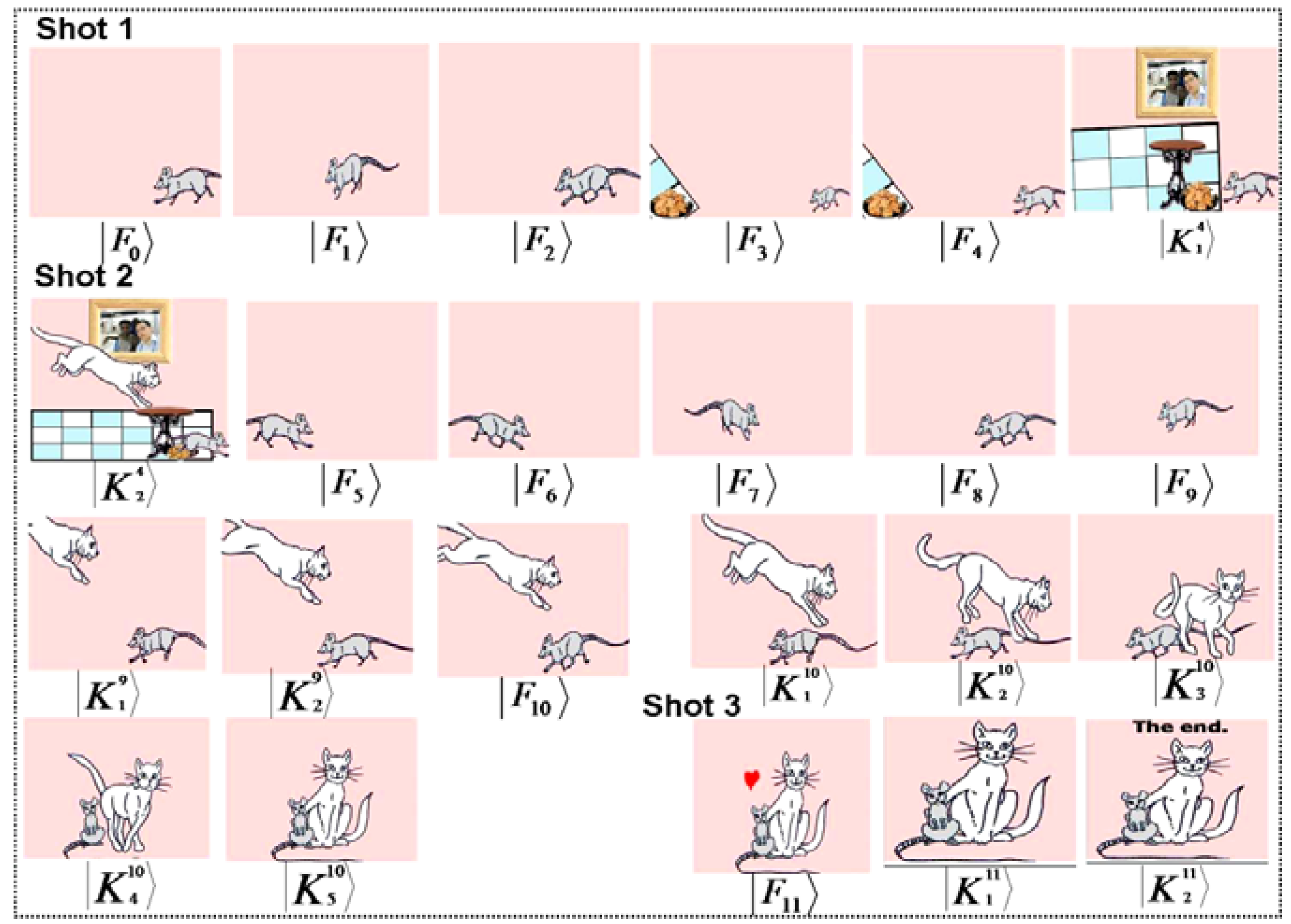
Figure 66. Key and makeup frames for the scene “The cat and mouse chase”. See text and [19] for additional explanation.

Figure 66. Key and makeup frames for the scene “The cat and mouse chase”. See text and [19] for additional explanation.

In the sequel, we present, albeit separately for each scene, an expansive discussion on the circuitry required to metamorphose the movie summary of each scene (i.e. the combination of key and makeup frames in Figure 65 and Figure 66) into a more detailed description that conveys the script to the audience. All the frames (makeup, key, and the viewing frames resulting therefrom) are of size 256×256. Hence, eight qubits (four for each position axis) are required to encode the position information, one qubit to encode the colour content, and another six qubits on the strip axis to encode the 40 key and makeup frames that make up the movie summary. Consequently, for brevity, we omit the final movie sub-circuits of the two scenes. The circuit elements of each sub-circuit interpolate the missing content between successive key frames of each scene.

6.4.1. Scene 1: The Lonely Duck Goes Swimming

As suggested by the title, the objective of the scene is to convey the bits and pieces of actions that show the duck right from when it leaves home (makeup frame $|K_1^0\rangle$), the various dialogues it encounters as it journeys to the stream for a swim (key frame $|F_0\rangle$ through to key frame $|F_4\rangle$), culminating in transformations on the movie summary to show it swimming. Finally, the scene ends with the duck’s homebound journey at around sunset. Broadly speaking, this scene can be divided into three parts. Consequently, we tailor our discussion on this scene along these three shots. All the movie operations in this scene comprise of SMO and GTQI transformations. These key and makeup frames are assumed to have been prepared and initialised in our movie strip.

From the content of this scene we can realise a total of 402 viewing frames as enumerated in the sequel.

In the first appearance in shot 1, we want to show the duck; its house, from a somewhat wide-angle view; and an impression of when the duck left home. A frame is prepared to convey these requirements. Going by our definitions and delineations between a key and makeup frame in subsection 6.2, a key frame may not capture all the required information. Consequently, the makeup frame $|K_1^0\rangle$ is prepared to do so. In subsequent frames, appropriate movie operations are applied in order to obtain the expanded description that seamlessly connects the content of the key and makeup frames in the shot. Where necessary, the shift steps are adjusted in order to depict the pace of the particular ROI for each key frame: the duck in $|F_0\rangle$; the dog, ball, and duck in $|F_1\rangle$; the ball and duck in $|F_2\rangle$; the ball in $|F_3\rangle$; and the dog and bird in $|F_4\rangle$. In addition to this, the shift steps are adjusted to overcome the effects of overflow in the new content obtained as discussed in subsection 6.3, specifically, Figure 48. In depicting the movements of the various ROI’s in each of the key frames, appropriate control-operations are applied on the position and strip axis in order to constrain the effect of the movie operations to the intended key frame and ROI. A total of 138 viewing frames were realised from the five key frames in this shot. The makeup frames $|K_1^0\rangle$ and $|K_2^0\rangle$ add a bit of realism to the scene by showing us from where and when the duck sets out for the swim and some of the dialogues it encounters on its way. These are crucial to conveying the content of this shot.

The first dialogue depicted in the second shot shows to the audience how the duck spends its time on reaching the stream. The gradual change in background from daylight to sunlight (between $|F_6\rangle$, $|K_1^6\rangle$ and $|K_1^6\rangle$) creates an impression about the duration of time it spends there. The key frames $|F_5\rangle$ and $|F_6\rangle$ together with the viewing frames obtained from them complete the dialogues in this shot. Meanwhile, the makeup frames $|K_1^4\rangle$, $|K_2^4\rangle$, $|K_1^6\rangle$, and $|K_1^6\rangle$ add realism to the content. Altogether, we realise 196 viewing frames by manipulating the key and makeup frames in this shot.

The last shot of this scene consists of (key and makeup) frames with the same background as those in shot 1 but at a different time. The intention is to show the duck on its homebound journey at sunset. The various transformations as discussed in shots 1 and 2 can be used in order to convey the required content. We assume no diversions as the duck heads home and that it does not run into the girl and her dog as in shot 1. From the key frames in this shot we realise the last 32 viewing frames of the scene.

6.4.2. Scene 2: The Cat and Mouse Chase

This scene depicts the dialogues between two traditional foes, a cat and a mouse. Contrary to expectations, however, the characters in this scene are the best of friends. This goes to buttress an earlier assertion that the script, which conveys the various actions and dialogues in the movie, is flexible to changes that convey whichever content is desired. The most important thing is how well the circuitor can study its content, and decide in liaison with the director, the appropriate key and makeup frames that will give an overview of this script.

From this content a more detailed content to efficiently translate the script is then realised. Such a summary for our scene entitled “The cat and mouse chase” that comprises of 23 key and makeup frames is presented in Figure 66.

The scene starts off with the first shot which comprises of five key frames and a makeup frame from which we would ordinarily realise 112 viewing frames. In order to create the impression of a running mouse, however, the shift steps have to be increased. In the end, using the factors enumerated earlier, we realise 75 viewing frames.

In the second shot, the traditional chase between the cat and the mouse ensues. Using the key frame $|K_2^4\rangle$, the impression of the cat pouncing on the mouse is created.

Sensing the imminent danger, we see the mouse running back towards the safety of its hole. In subsequent key frames $|F_6\rangle$ through to $|F_9\rangle$ we see the actions of a frightened and confused mouse: first running toward its hole (key frames $|F_5\rangle$, $|F_6\rangle$ and $|F_7\rangle$), then turning back toward the cat (key frames $|F_8\rangle$ and $|F_9\rangle$). The control-conditions are crucial to effectively convey the different actions of the cat and mouse in key frames $|F_{10}\rangle$. This key frame and the eight viewing frames we obtain from it when combined with the subsequent makeup frames $|K_1^{10}\rangle$, $|K_2^{10}\rangle$, $|K_3^{10}\rangle$, $|K_4^{10}\rangle$, and $|K_5^{10}\rangle$ convey how the cat and mouse finally meet. Instead of the cat pouncing to eat up the mouse, using key frame $|F_{11}\rangle$, the cordial relationship between these traditional foes is conveyed to the audience. Finally, by assuming this is the last scene of the movie, makeup frames $|K_1^{11}\rangle$ and $|K_2^{11}\rangle$ are used to end the scene as seen in Figure 66.

From these two scenes, a key advantage of the proposed framework has become manifest. Using only 40 makeup and key frames, a movie comprising 597 frames is realised. Such an astute manipulation of the abstract content of the movie guarantees that the initial cost of producing quantum movies will always be less than the traditional classical versions of the same movie. This is evident because the classical version of our movie “The cat, the mouse, and the lonely duck” would require a 597-frame long strip to realise. This we have accomplished using only 40 key and makeup frames.

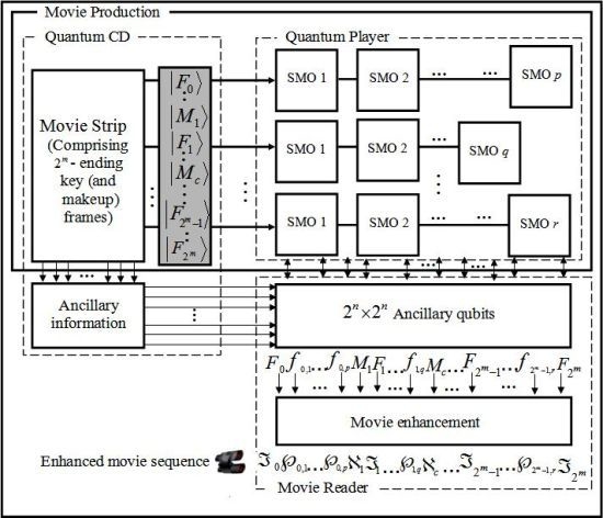
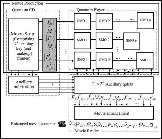
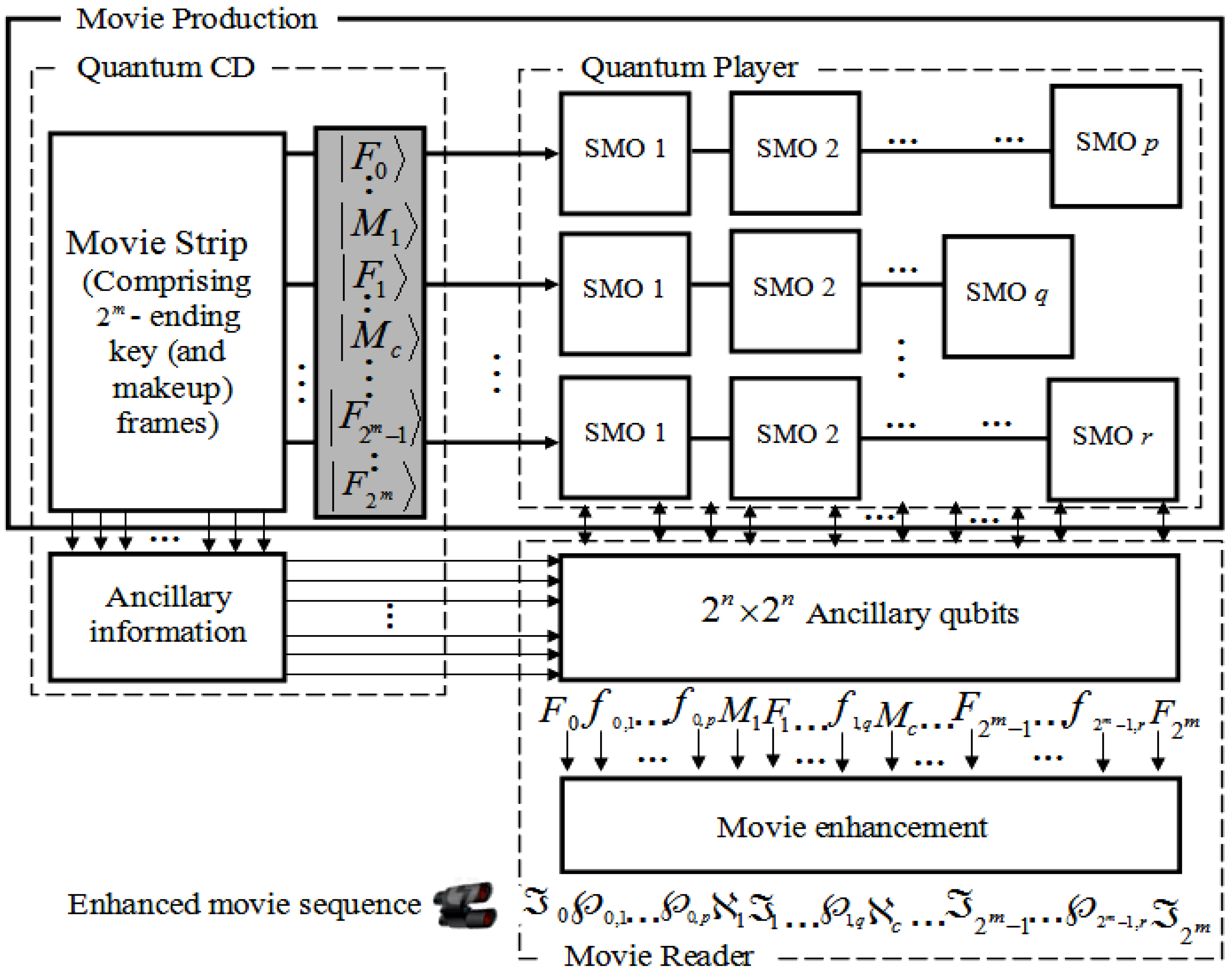
We conclude by presenting the overall framework to represent and produce the quantum movies as shown in Figure 67. This is achieved by concatenating the three movie components discussed in this section into a single gadget. Based on our proposed framework, the quantum CD and player facilitate the capture of the contents of the key frames and then transform them into viewing frames which together combine to represent the bits and pieces of action required to convey the script to the audience.

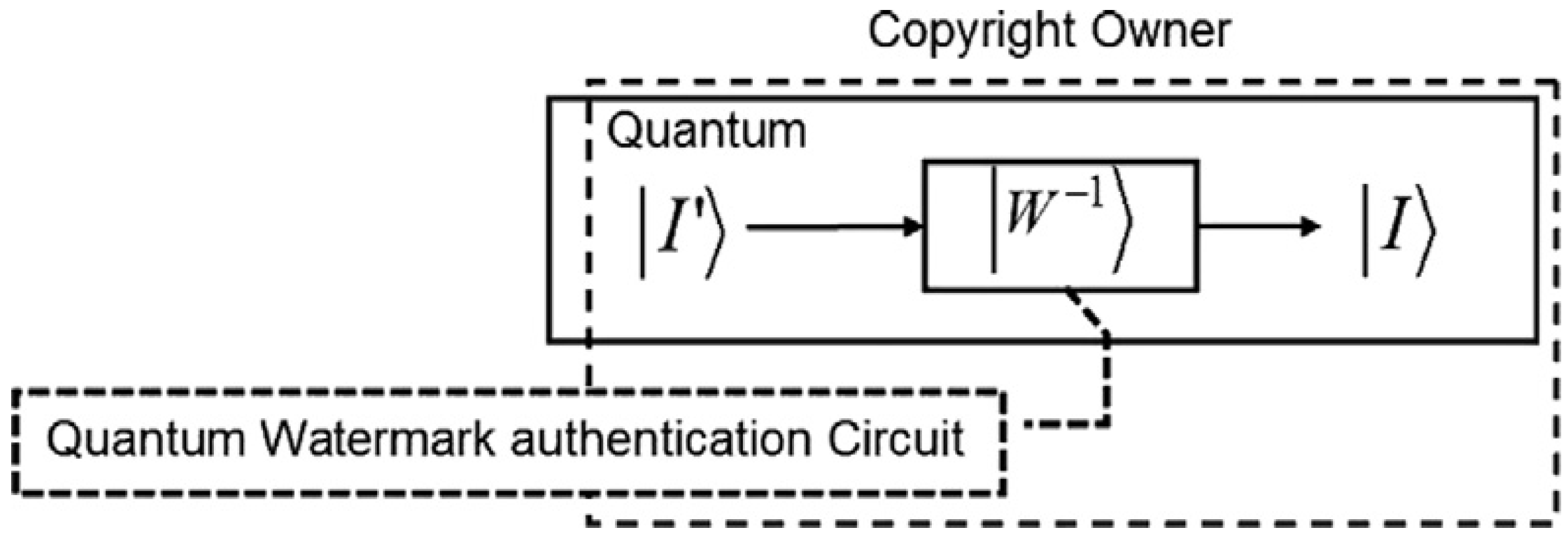
The constraints imposed by the quantum-classical interaction of data, more specifically, quantum entanglement and superposition, ensure that the content as produced and manipulated by the quantum CD and player cannot be viewed by the audience. The movie reader is therefore used to “decode” these frame (i.e. key, makeup, and viewing) contents in such a way that the earlier constraints are not unsettled.

It should be emphasised that while the components have been designed as standalones, it is assumed interaction between them is both feasible and mandatory. Notwithstanding the interaction, however, the standalone feature of the three movie components guarantees multiple usage of the data stored and processed by the various components.

The movie enhancement stage of the movie reader is added to show the need to enhance the content of each frame before final display to the audience. This stems from the fact that we have focused our colour processing tasks mainly in terms of the binary states $|0\rangle$ and $|1\rangle$. This agrees with the intuition in classical image processing.

Numerous classical technologies which can be easily co-opted at this stage of the proposed framework abound [30]. In addition, the enhancement stage is responsible for tuning the movie sequence to the appropriate frame transition rate (usually 25 frames per second) to be broadcast to the audience. This enhanced content of the movie is given by the sequence:

$$\begin{array}{l}M={\xi }_0\left({\iota }_{0,0},{\iota }_{0,1},\hspace{0.17em}\cdots ,\hspace{0.17em}{\iota }_{0,p}\right)\hspace{0.17em}{\kappa }_1^0{\xi }_1,\hspace{0.17em}\cdots ,\hspace{0.17em}{\xi }_2^{m-1}\\ \hspace{0.17em}\hspace{0.17em}\hspace{0.17em}\hspace{0.17em}\hspace{0.17em}\hspace{0.17em}\hspace{0.17em}\hspace{0.17em}\hspace{0.17em}\hspace{0.17em}\hspace{0.17em}\hspace{0.17em}\hspace{0.17em}\times \left({\iota }_{2^m-1,0},\hspace{0.17em}{\iota }_{2^m-1,1},\hspace{0.17em}\cdots ,{\iota }_{2^m-1m-1,q}\right)\hspace{0.17em}{\xi }^{2^m}\end{array}$$

(63)

Figure 67. Framework for quantum movie representation and manipulation.

Figure 67. Framework for quantum movie representation and manipulation.

6.5. Conclusions on Framework to Represent and Produce Movies on Quantum Computers

By generalising the criteria to realise a quantum system to include preparation, manipulation, and measurement, a standalone quantum device is proposed to represent the various requirements of each criterion. A quantum CD is proposed for the preparation criteria, wherein, the broad content or key frames to convey the movie script are encoded, prepared, and initialised as a large superposition of multiple key frames called the strip. The quantum player utilises a set of SMOs, GTQI, and CTQI operations to manipulate these key frame contents in order to interpolate the missing content between successive key frames. These operations as required to effectively depict the movements and motions in the scenes and shots of the movie combine to produce the movie circuit. The transformed version of each key frame produces a viewing frame at every measurement layer of the movie circuit. Where certain content in a scene cannot be realised by transforming a key frame, makeup frames are included to make up for the hitherto unrepresented content. The classical sequence comprising of the key frames, makeup frames, and the interpolated viewing frames in between them are retrieved by the movie reader. At appropriate frame-to-frame transition rates, this sequence conveys the shots and scenes that depict the content of the movie to the audience. Three elaborate examples were presented to demonstrate the feasibility of the proposed framework, particularly with regards to the quantum player. Concatenated, these components together facilitate the proposed framework for quantum movie representation and production, thus, opening the door toward manipulating quantum gates and circuits aimed at applications for information representation and processing.

7. Concluding Remarks and Future Perspectives

The growing desire for faster, smaller and more sophisticated data communications and networking has made us more vulnerable to the risk of knowledge, identity, and information theft than at any other period of human civilisation [1].

As the speed of our present computing resources doubles every 18 months, its size is expected to shrink by half, implying that at the turn of the next decade the size of the microprocessor would be approaching the atomic scale. At such a size, the laws of physics that govern the way this computing hardware are to process information may become infeasible or at best inefficient, hence, the need for a shift to a new, faster and more efficient computing paradigm - quantum computing. On this new framework the requirements to perform any information processing task will be dictated within the confines of quantum mechanics, which is endowed with a few properties for which there are no analogues on the present paradigm. These properties are partly responsible for some of the fascinating results realised when traditional information processing resources used to mimic the behaviour of the quantum mechanical information carrier.

Whether as complete computing units or as devices co-opted to complement traditional computing resources, quantum computing hardware are sure to play some role in the next generation of super-fast, efficient and secure computing gadgets. This is even more so, since image and video processing applications and devices are now a part of our daily lives. The thought of our lives without these, often, tiny little gadgets that capture, store, process and share images and video is both petrifying and unwarranted. In addition, it is estimated that this industry is worth billions of US dollars in annual revenue. Since it is inevitable that we will soon reach the limits of today’s computing hardware, and in order to sustain the current pace of advancement in image and video processing, it has become imperative that we consider a new set of hardware otherwise some of the applications and tasks we are used to today may no longer be feasible.

The main purpose of this review is to gather all the related literature tailored the execution of image and video processing applications and tasks on the quantum computing framework into a single source. This could then be formulated to function alongside the traditional ones that are available today. Thus, ensuring some measure of continuity in the manner and sophistication with which we process images and video. Specifically, our review is focussed on algorithmic frameworks and protocols on images that are encoded as FRQI states.

Based on the motivations enumerated above, the review started with the fundamental requirement that would facilitate image processing on quantum computers, i.e. a representation for an image that can with withstand the intricacies inherent to the quantum computing framework. A new proposal of a flexible representation of quantum (FRQI) images was proposed in Section 2 to allow unitary transformations to apply on quantum images.

The proposed representation captures and stores two fundamental information about the colour and position of every point in an image (as a normalised quantum state) [1,11,12].

Various types of transformations to focus on changing information about both colour and position in the images, named geometric (GTQI) and colour (CTQI) transformations, were then proposed based on the FRQI representation [1,30,31,32]. The transformations serve as foundation blocks for algorithms that would facilitate higher-level quantum image processing applications.

Exploiting the intuitive and flexible features of the FRQI representation and transformations on it, two mathematical schemes and algorithms that determine the composition of quantum circuit elements required to modify the content of a cover image in order to watermark, authenticate and recover unmarked versions of the cover images are proposed.

In the first scheme [1,17,18], a secure, keyless, and blind watermarking and authentication strategy for images on quantum computers, WaQI, is proposed based on restricted geometric transformations on the content of the cover image. In contrast with conventional digital watermarking techniques where geometric transformations on the contents of an image are considered undesirable, the proposed WaQI scheme utilises the restricted variants of the quantum versions of these transformations as the main resources that dictate the composition of a bespoke watermark map, which translates of the watermark embedding and authentication circuits. This scheme provides the framework for representing two or more quantum data as a single quantum circuit and opens the door for other applications aimed at their protection.

The second scheme [1,20] proposes appropriate modifications to the FRQI representation in order capture greyscale versions of the input quantum images and watermark signals.

By focusing on transformations on the single qubit that encodes the chromatic information about FRQI images, the proposed scheme is used to execute a two-tier watermarking and recovery of unmarked greyscale images on quantum computers. The hitherto inaccessible data from a quantum image-watermark pair is extracted from their classical versions using which two quantum sub-circuits are used to execute the bi-level watermark embedding comprising of changes that (1) embed a visible and translucent watermark logo in a predetermined sub-area of the quantum replica of the cover image, and (2) modify the remaining content of the cover image in a manner dictated by the watermark signal, so that the resulting distortions on the watermarked image are not easily discernible.

The ability to employ classical computing resources in order to simulate the image-watermark pairs and the various sub-circuits required to obtain the marked and unmarked images demonstrates the feasibility of the proposed schemes when the necessary quantum hardware are realised leading to safeguarding of quantum data from unauthorised reproduction and confirmation of their proprietorship in cases of dispute.

Furthermore, by adopting a generalisation of the DiVincenzo criteria [33] for the physical realisation of quantum devices in tandem with the FRQI representation, a standalone component each, was proposed to prepare, manipulate, and measure the various content required to represent and produce movies on quantum computers [1,19]. The Quantum CD: encodes, prepares, and initialises the broad content or key frames conveying the movie script. The Quantum Player uses the simple motion operations to manipulate the contents of the key frames in order to interpolate the missing viewing frames required to effectively depict the shots and scenes of the movie. The Movie Reader utilises the ancilla-driven quantum computation to retrieve the classical movie sequence comprising of both the key—and viewing—frames for each shot. At appropriate frame transition rates, this sequence creates the impression of continuity in order to depict the various movements and actions in the movie. Three well thought-out examples demonstrate the feasibility of the proposed framework. Concatenated, these components together facilitate the proposed framework for quantum movie representation and production, thus, opening the door towards manipulating quantum circuits aimed at applications for information representation and processing.

Finally, the ultimate target is how to breathe life into all this algorithms and protocols. Therefore, it would be worthwhile to consider the physical realisation, even if abecedarian in nature, of some of the image processing schemes reviewed in this work. One possible direction involves characterising the information carrier to encode the FRQI images as photons, from which a compendium comprising of an assessment of the current state of photonic quantum technologies as required to facilitate FRQI image processing applications was presented in [1,21]. It was noted therein that there are numerous challenges that may impede the realisation of the necessary hardware to implement most of the applications proposed in this work. Modifications and extensions to the available technologies [77,78,79,80,81] that are considered apt in order to overcome likely challenges that may encumber the realisation of meaningful image processing tasks were also suggested. Overall, the realisation of components to execute two-qubit control condition operations [80] presents the most daunting yet vital steps in the march towards realising application-specific photonic quantum hardware for FRQI image processing.

As emphasised throughout this review, the realisation of more advanced classical-like image processing tasks using the FRQI encoded quantum images depends on how we can further exploit the flexibility inherent to the FRQI representation in order to come up with new transformations on the colour, position, or both colour and position information that the FRQI representation captures. Discovering new applications is dependent on our ability to come up with new transformations. In line with this, the research presented in this work can be extended along the under-listed directions.

As presented in Section 3 and Section 5, there is the need to consider extensions to improve the FRQI representation either along the line of the chromatic content (such as the greyscale version of FRQI quantum images discussed in Section 4) it encodes or in order to allow the capture of multiple images as in the strip or movie FRQI that was introduced in Section 5. One such idea is that to represent the FRQI image in terms of RGB colour components as suggested in [1,22]. This has the potential to realise applications that target any of these colour channels. However, there are still many obstacles that need be to overcome, such as an analysis of how to curtail the likely complexity of new transformations and the possibility of realising the hardware to execute these more difficult transformations.

As highlighted earlier, new transformations are very important for building new and efficient applications. There are some efficient transformations already available on the quantum computation framework (such as Fourier, discrete cosine, and wavelet transformations) whose classical equivalents have proven very useful in classical image processing. Especially considering the role the classical equivalents have played in enhancing classical image processing, it appears worthwhile to explore the possibility of extending these quantum versions in order to enhance the FRQI quantum image processing applications proposed in this work.

The extensions suggested above are all focussed on single images. There are interesting questions regarding the nature of operations required to process the information encoded in multiple images such as image matching and image searching on a dataset of FRQI quantum images states [23,24]. These are sure to open new directions for quantum image processing in general.

In Section 3 and Section 4 the assumption was made that all the hardware used to realise our proposed WaQI and WaGQI schemes were fault-tolerant and therefore free of errors. Although this assumption is tenable, it does not appear practical especially in quantum computing hardware where the system must be isolated from the outside world. It is therefore, imperative to consider schemes were the whole framework is embedded with capabilities for noise limitation and error-correction.

Still on the issue of errors, arising from often bad correlation between the values obtained and the actual visual quality of the watermarked images, the use of the PSNR as an evaluation metric for evaluating the fidelity of watermarked data [82,83,84,85,86,87] on the quantum computing paradigm deserves further attention. A new wholly quantum metric capable of incorporating numerics to atone for the likely presence of error and noise in the watermarked quantum data should be proposed.

The proposed framework for quantum movie production presented in Section 5, although a very modest attempt is at the stage present day movies were in the latter periods of the 19th century, hence, there are numerous directions that the proposal can be improved on.

First of all, the standalone nature of the three devices as proposed in the framework makes their separate implementation worth pursuing. With this, come the separate challenges geared towards improving the performance of each device. To do this, starting with the Quantum CD, as with ongoing research to realise a physical quantum computer using different technologies, the inherent difficulties in preparing and initialising the movie strip must be overcome.

The Quantum Player poses the most challenges in terms of improving the performance of the proposed framework. Accordingly, this work is being extended in the following directions. To start with, a modification to the mFRQI representation is being sought to make it more practical in terms of mimicking real life movie requirements such as: being able to isolate any irregular $n\times m$ ROI from a larger $n\times n$ input key frame; or, showing an overlap of two or more objects: such as a man holding a ball, i.e. occlusion; and in order to more practicable, the scheme should be capable of showing objects in their true geometry; round, oval etc. Projective transformations on the FRQI quantum images will provide a fresh perspective to transform the FRQI state of the key frames in order to improve the depiction of the movements in the movies and is currently being pursued.

Finally, the cost in terms of the basic gates of the movie reader as proposed here needs to be reviewed. This can be addressed by formulating circuits that decompose the control-operations required at each layer of the ancillary measurement. Ultimately, as it was with the classical movies, sound would have to be incorporated in order to produce real talking quantum movies. However, to do that a representation for sound on a quantum computer must be formulated before its integration into the silent quantum movie as proposed here.

The work presented in this review could also be used to improve other protocols that, although not covered in the review, adopt the FRQI representation to encode and manipulate the content of their images. For example, the scheme to compare two quantum images (each an FRQI image) in [24], which was based on the cosine function of pixel difference at every position of the images, can be improved by applying the quantum Fourier or wavelet transform [16,24]. Such comparison could then be used to determine the image with highest similarity to a reference image as one would quantum watermarking [1,17,18,19]. By further exploiting the parallelism inherent to quantum computation, it is envisaged that quantum image database search will be significantly faster than those on classical computers. Thirdly, besides the ability to measure the difference between the original image and the watermarked image which was suggested earlier, the proposed image similarity assessment in [24] could also be applied to the quantum movie [1,20] in order to enhance the smoothness and continuity of the frame to frame transition between scenes, and also in the production of quantum movie trailers. These extensions will open new directions for efficient image and video processing using quantum computing hardware.

The use of the FRQI representation to encode images together with the various algorithmic frameworks to manipulate its content and directions suggested to extend and improve these protocols as detailed in this review provide the road-map towards the realisation of secure and efficient image and video applications on quantum computers.