Fluctuations in the Energetic Properties of a Spark-Ignition Engine Model with Variability

Abstract

We study the energetic functions obtained in a simulated spark-ignited engine that incorporates cyclic variability through a quasi-dimensional combustion model. Our analyses are focused on the effects of the fuel-air equivalence ratio of the mixture simultaneously over the cycle-to-cycle fluctuations of heat release ($Q_R$) and the performance outputs, such as the power (P) and the efficiency (η). We explore the fluctuant behavior for $Q_R$, P and η related to random variations of the basic physical parameters in an entrainment or eddy-burning combustion model. P and η show triangle shaped first return maps, while $Q_R$ exhibits a structured map, especially at intermediated fuel-air ratios. Structure disappears to a considerable extent in the case of heat release and close-to-stoichiometry fuel-air ratios. By analyzing the fractal dimension to explore the presence of correlations at different scales, we find that whereas $Q_R$ displays short-range correlations for intermediate values of the fuel ratio, both P and η are characterized by a single scaling exponent, denoting irregular fluctuations. A novel noisy loop-shaped P vs. η plot for a large number of engine cycles is obtained. This plot, which evidences different levels of irreversibilities as the fuel ratio changes, becomes the observed loop P vs. η curve when fluctuations are disregarded, and thus, only the mean values for efficiency and power are considered.

1. Introduction

In a typical internal combustion engine, several thousands of cycles are performed in a minute, but several theoretical and experimental studies support the existence of significant variations from one cycle to the next. Those variations can be found, for example, in the combustion heat and in the in-cylinder pressure [1,2,3]. Many thermal and mathematical phenomena support so-called cyclic variability (CV), which is associated with a very complex dynamical behavior. In fact, during the last years, many researchers have investigated CV either experimentally or by means of theoretical methods, including nonlinear dynamics and chaos theory [1,4,5]. From a practical engineering viewpoint, monitoring cycle-to-cycle variations can enable closed-loop control over engine parameters, such as fuel metering or spark timing, in order to reduce fuel consumption and increase power output or other performance records [6,7]. Reduction of cycle-to-cycle variations could allow the engine to operate under average conditions closer to the limiting ones, improving performance related to driveability, increased power output, overall efficiency and reduced environmental impact [8,9].

Among the phenomena that cause cyclic variability, turbulent combustion is recognized as one of the most important. Briefly, we also remark on those associated with the turbulence existing in the process of fuel-air intake, together with the overlapping in the opening times of the intake and exhaust valves, which leads to the fact that not all of the gases in the cylinder are expelled during the exhaust process. This residual mixture includes combustion products and some unreacted fuel and air. Thus, the reactive mixture is different in each cycle of a sequence and, therefore, the combustion heat also changes form cycle to cycle. Small changes in the atmospheric pressure and in the chemical composition of the air can also produce minor changes in the combustion heat. In fact, the fluctuant combustion heat produces changes in all thermodynamic states, followed by the working fluid, along any thermal cycle, representing an internal combustion engine. Therefore, this provokes changes in performance quantities, such as power output and efficiency. For analyzing this kind of fluctuation, many authors have reported extensive work relative to CV in spark-ignition engines by means of different statistical methods, such as return maps, recurrence maps, correlation coarse-grained entropy and sample entropy [1,10,11,12,13]. Recently, Curto-Risso et al. [14] and Sen et al. [2,5] investigated the complex dynamics of cycle-to-cycle heat release variations in a spark-ignition engine by using fractal and multifractal methods.

During the last 30 years, numerical simulation models have been an essential technique in the development of modern and efficient spark ignition engines. Most simulations take as a starting point the air standard Otto cycle, but they also incorporate submodels for the gas flows through the valves, heat losses through the cylinder walls, realistic friction models, turbulent combustion dynamics and several others [15].

The so-called multi-dimensional models solve a complicated set of partial differential equations by dividing the volume of the combustion chamber in a grid. Multi-dimensional models have a complex implementation and require powerful computation resources (that make it difficult to calculate more than a few cycles). The obtention of the requested information is associated with several uncertainties. On the contrary, in zero-dimensional (thermodynamic) models, all variables are averaged over a finite volume, and combustion is approached by means of an empirical correlation. For zero-dimensional models, the main drawbacks are oversimplification and the absence of spatial resolution in the combustion process. Another numerical schemes in between is the so-called quasi-dimensional simulation. It improves the zero-dimensional ones with the assumption of an approximately spherical flame front and the incorporation of two additional differential equations that describe the evolution of combustion. Therefore, after establishing some simplifying hypotheses, these allow for the implementation of simple geometries and turbulent combustion models. Quasi-dimensional models have shown their capability to reproduce and analyze the experimentally observed cycle-to-cycle variations in parameters, such as the indicated mean effective pressure (IMEP), in-cylinder pressure (maximum or at a given crank angle), ignition delay, mass fraction burnt or heat release during combustion [8,16]. They bear the advantage of a low computational cost and, moreover, allow a direct analysis of the relationships between basic physical parameters and variability. Quasi-dimensional models solve explicit differential equations for the evolution of burned and unburned masses of the fuel-air mixture during combustion, making the hypothesis that the flame front is roughly spherical [17]. Besides, in those models, two ordinary differential equations for the pressure and the temperature of the gases inside the cylinder (raised from the basic laws of thermodynamics) are solved for each time step or crankshaft angle.

The main goal of this paper is to show a probabilistic interpretation of CV phenomenology in reference to the most important energetic indicators for a spark-ignition engine. Special emphasis is put on the behavior of heat release, power output and efficiency, as well as the power versus efficiency plots. In particular, in thermodynamic optimization methods, these plots are widely used to get unified insights about the optimum performance regimes, widely acknowledged as those ranging between maximum power and maximum efficiency [18]. The structure of the paper is as follows: in Section 2, we give a brief background of the simulated model we use to evaluate the effects of the fluctuations [14,16]; Section 3 is devoted to presenting the results for the main statistical parameters characterizing the energetic properties; and in Section 4, we analyze the performance output functions and the power-efficiency plots. Finally, we summarize the main results and present conclusions of the work.

2. Simulated Model: Theoretical Background

We consider an internal combustion reciprocating engine operating on four strokes per cycle. Each cylinder performs four strokes of its piston (that corresponds to two revolutions of the crankshaft) to complete the series of events that lead to one power stroke. Our numerical model is based upon the first principle of thermodynamics for open systems expressed as a differential set of equations. We assume a two-zone model for combustion, thus discerning between burned (b) and unburned gases (u). Except during combustion, the working fluid could be considered as an adiabatic mixture of both gases. We suppose all gases as ideal with temperature, T, and pressure, p, independent gas constant, $R_u$ or $R_b$, a constant fuel-air ratio, $\varphi$, and except in combustion, only enthalpy changes associated with temperature variations.

A differential equation for either burned or unburned gases temperature inside the cylinder can be written, except in the combustion period (that will be considered later on) as in [19]:

$$\frac{dT}{dt}=\frac{1}{\left(m_u{c}_{p,u}+m_b{c}_{p,b}\right)}\left[{\dot{Q}}_u+{\dot{Q}}_b+{\dot{m}}_{\mathrm{in}}{h}_{\mathrm{in}}+{\dot{m}}_{\mathrm{ex}}{h}_{\mathrm{ex}}-{\dot{m}}_u{h}_u-{\dot{m}}_b{h}_b+V\frac{dp}{dt}\right]$$

(1)

In absence of combustion, the system can be considered as an adiabatic mixture, and in that case, the equations of temperature are the same for both gases. The term, ${\dot{m}}_u{h}_u+{\dot{m}}_b{h}_b$, corresponds to enthalpy changes of the gas mixture inside the cylinder associated with mass changes, while ${\dot{m}}_{\mathrm{in}}{h}_{\mathrm{in}}$ and ${\dot{m}}_{\mathrm{ex}}{h}_{\mathrm{ex}}$ correspond to the enthalpy changes associated with intake or exhaust processes. ${\dot{m}}_{\mathrm{in}}$ and ${\dot{m}}_{\mathrm{ex}}$ can be positive or negative, depending on the relative pressures between the cylinder interior and the intake or exhaust pressures. ${\dot{Q}}_u$ and ${\dot{Q}}_b$ correspond to the heat loss of unburned or burned gases. In the processes where unburned gases inside the cylinder do not exist, $m_u=0$ and, then, ${\dot{Q}}_u=0$, and the same applies for the burned gases. Therefore, each term for u or b can appear or not in the equation, depending on the stroke (and, similarly, for the terms with the subscripts, $\mathrm{in}$ or $\mathrm{ex}$, during the strokes, the system is closed). The initial values are given by the external conditions.

For pressure, with the same arguments as for temperature, the corresponding equation can be written as [20]:

$$\begin{array}{cc}& {\displaystyle \frac{dp}{dt}=[p\left(\frac{{\dot{m}}_u}{{\rho }_u}+\frac{{\dot{m}}_b}{{\rho }_b}-\frac{dV}{dt}\right)+}\end{array}$$

$$\begin{array}{cc}& {\displaystyle +\zeta \left({\dot{Q}}_u\dot{+}{Q}_b+{\dot{m}}_{\mathrm{in}}{h}_{\mathrm{in}}+{\dot{m}}_{\mathrm{ex}}{h}_{\mathrm{ex}}-{\dot{m}}_u{h}_u-{\dot{m}}_b{h}_b\right)]\frac{1}{\left[V\left(1-\zeta \right)\right]}}\end{array}$$

(2)

with

$$\zeta =\frac{V}{{\displaystyle \frac{V_u{c}_{p,u}}{R_u}+\frac{V_b{c}_{p,b}}{R_b}}}$$

(3)

Thus, except for combustion, Equation (1) and Equation (2) are valid at any other moment of the system evolution, including the overlapping period. Throughout combustion, we consider two control volumes, for burned or unburned gases, separated by the propagating flame front. This leads to different temperature equations for unburned and burned gases. Changes in the chemical enthalpy of fuel are considered. Thus, as in other two-zone models [21], during the combustion period, the equations giving the time evolution of $T_u$, $T_b$ and p can be written as:

$$\frac{d{T}_u}{dt}=\frac{{\displaystyle {\dot{Q}}_u+V_u\frac{dp}{dt}}}{m_u{c}_{p,u}}$$

(4)

$$\frac{d{T}_b}{dt}=\frac{{\displaystyle {\dot{Q}}_b+{\dot{m}}_b\left(h_u-h_b\right)+V_b\frac{dp}{dt}}}{m_b{c}_{p,b}}$$

(5)

$$\begin{array}{}& \hfill \frac{dp}{dt}=& {\displaystyle [p\left({\displaystyle \frac{{\dot{m}}_b}{{\rho }_b}+\frac{{\dot{m}}_u}{{\rho }_u}-\frac{dV}{dt}}\right)+\frac{{\dot{Q}}_u{R}_u}{c_{p,u}}+}\hfill (6)& & {\displaystyle +\left({\dot{Q}}_b+{\dot{m}}_b\left(h_u-h_b\right)\right)\frac{R_b}{c_{p,b}}]{\left({\displaystyle V-\frac{V_u{R}_u}{c_{p,u}}-\frac{V_b{R}_b}{c_{p,b}}}\right)}^{-1}}\hfill \end{array}$$

Initial values for $T_u$ and p at the beginning of combustion are given by Equation (1) and Equation (2), whereas for $T_b$, the initial value is calculated as the adiabatic flame temperature (at constant pressure). The different terms included in all the thermodynamic equations above require one to be specified in the different steps of the system evolution to account for the physical nature of the processes, which have to be adequately modeled.

In order to follow the evolution of the mass of the unburned and burned gases during combustion, we make use of the turbulent quasi-dimensional model developed by Keck [22] and extended by Beretta [23]. The burning of the cylinder charge is considered as a turbulent flame propagation process. During this process, because of turbulence, unburned eddies of characteristic length, $l_t$, are entrained into the flame zone at a velocity, $u_t+S_l$, where $u_t$ is the characteristic speed (similar to the local turbulence intensity [17]) and $S_l$, the laminar flame speed. Then are burned at velocity $S_l$ in a characteristic time, ${\tau }_b=l_t/S_l$. The laminar flame speed, $S_l$, depends on the thermodynamic conditions, but also on the fuel-air equivalence ratio and on the mole fraction of gases in the chamber after combustion. In other words, $S_l$ connects combustion dynamics and the proportion of residual gases in the cylinder after the previous event (the memory of the chemistry of combustion).

Models like this one are usually called entrainment or eddy-burning models. Thus, combustion is described by solving this set of ordinary differential equations:

$$\begin{array}{}& \hfill {\dot{m}}_e& =A_f{\rho }_u\left(u_t+S_l\right)\hfill (7)& \hfill {\dot{m}}_b& =A_f{\rho }_u{S}_l+\frac{\left(m_e-m_b\right)}{{\tau }_b}\hfill \end{array}$$

where $m_e$ denotes the total mass inside the flame front, burned gas and unburned eddies. $A_f$ is the area of the spherical flame front. During combustion, these equations are coupled with the thermodynamic ones, Equations (4)–(6). Laminar burning speed is obtained from Gülder’s model [24] and $u_t$, $l_t$ from the empirical correlations built up by Keck [22]. $A_f$ is calculated from its radius, assuming a spherical flame front, and the radius from the volume of the gases inside the flame front, $V_f$, was calculated following Bayraktar [21].

Our study will only be concerned with the stationary evolution of the cycle at a fixed angular velocity. Thus, we do not include in the set of differential Equations (1)–(6) the mechanical equation for the relationship between the angular velocity and the forces on the piston. The heat transfer between the gas and the cylinder internal wall was assumed to follow Woschni’s correlation [25]. For engine friction, the model proposed by Barnes-Moss [17], which includes linear and quadratic terms on the engine speed, particularized for a single cylinder engine, is assumed. The friction forces appear on the calculation of the net work as: $\left|W\right|=|W_{\mathrm{gas}}|-|W_{\mathrm{fric}}|$. The power output is calculated by simply dividing the net work by the total time duration of the cycle. We have shown in previous works [19,26] that the comparison of the output parameters (power, efficiency, heat release, etc.) predicted from our model with experimental results is fairly good. Further details of the simulations and the corresponding running parameters can be found in those papers.

Together with gas mixture motion, turbulence during combustion and the homogeneity of the mixture composition near the spark plug, memory effects are considered by several authors as the main physical ingredients of cyclic variability [8,27]. Our recent studies [16] have shown that the incorporation of stochastic fluctuations in $l_t$ by fitting experimental results on combustion [23] allows us to reproduce the main characteristic of heat release fluctuations that is shown in the experimental works. The model also reproduces the main features of heat release cyclic variability when compared with experiments, as well as the evolution with the fuel ratio of the statistical parameters characterizing heat release time series and the corresponding return maps [16]. Furthermore, a fractal and a multifractal analysis of heat release was performed in [14].

As a summary of the theoretical section, it is important to note that in our dynamical system, the coupled ordinary differential equations for pressure and temperature are, in turn, coupled with two other ordinary differential equations for the evolution of the masses during combustion. All these variables evolve with time or with the crankshaft angle. As recently shown, this deterministic scheme does not reproduce the experimental characteristics shown by heat release fluctuations. The incorporation of stochastic fluctuations on the characteristic length of unburned eddies during combustion, $l_t$, is essential to reproduce the main features of heat release time series and their evolution with the fuel/air equivalence ratio [14,16].

Table 1. Geometrical characteristics of the cylinder considered for the simulations and other running parameters [16,19,23].

a, crank radius	44.45 mm
$n_v$, number of pairs of valves	1
l, connecting rod length	147 mm
$V_0$, clearance volume	1.05 × 10−4 m3
r, compression ratio	7.86
B, bore	101.6 mm
${\phi }_0$, spark angle	330.0°
μ, friction coefficient	16.0 kg/s
$C_D$, discharge coefficient	0.6
$p_{\mathrm{in}}$, intake pressure	0.72 × 105 Pa
$T_{\mathrm{in}}$, intake temperature	350.0 K
$p_{\mathrm{ex}}$, exhaust pressure	1.05 × 105 Pa
$T_{\mathrm{ex}}$, exhaust temperature	600 K
$T_w$, cylinder internal wall temperature	600 K
Heat transfer model	Woschni

Table 1. Geometrical characteristics of the cylinder considered for the simulations and other running parameters [16,19,23].

a, crank radius	44.45 mm
$n_v$, number of pairs of valves	1
l, connecting rod length	147 mm
$V_0$, clearance volume	1.05 × 10−4 m3
r, compression ratio	7.86
B, bore	101.6 mm
${\phi }_0$, spark angle	330.0°
μ, friction coefficient	16.0 kg/s
$C_D$, discharge coefficient	0.6
$p_{\mathrm{in}}$, intake pressure	0.72 × 105 Pa
$T_{\mathrm{in}}$, intake temperature	350.0 K
$p_{\mathrm{ex}}$, exhaust pressure	1.05 × 105 Pa
$T_{\mathrm{ex}}$, exhaust temperature	600 K
$T_w$, cylinder internal wall temperature	600 K
Heat transfer model	Woschni

All the results we present were obtained using isooctane as fuel. Details on the chemical reactions and assumptions on the calculation of residual gas fractions can be found in [16]. A summary of the geometrical characteristics of the cylinder, as well as some running parameters of the simulations are contained in Table 1 [16,19,23]. All the results obtained were performed over 10⁴ engine cycles, except when explicitly mentioned.

3. Energetic Properties with Variability

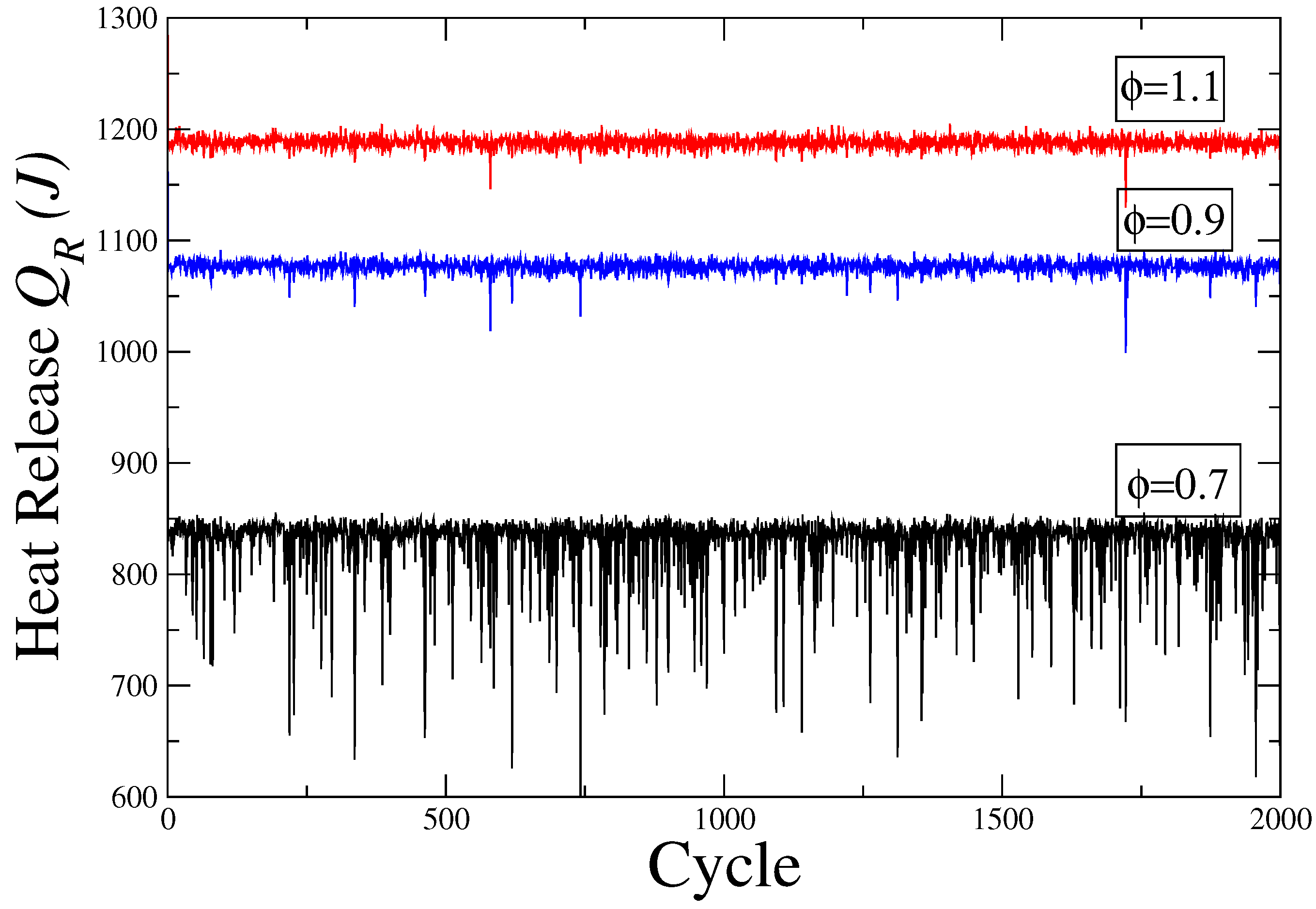
Heat release during combustion, $Q_R$, is numerically evaluated through the first principle of thermodynamics for open systems, separating the heat release, $\delta Q_R$, internal energy variations associated with temperature changes, $dU$, net work output (excluding friction forces), $\delta W$, and heat transfers from the working fluid to the cylinder walls, $\delta Q_l$: $\delta Q_R=dU+\delta W+\delta Q_l$. Internal energy and heat losses include terms associated with either burned or unburned gases. The net heat release during the whole combustion period is calculated by simple integration over that period.

Representative cases of the evolution in time of heat release, $Q_R$, are presented in Figure 1 for three values of the fuel ratio, $\varphi$. A noisy behavior is observed, with a decreasing amplitude of the fluctuations of $Q_R$ as the fuel ratio is close to unity. This noisy evolution is due to the introduction of a stochastic term in the characteristic length of the unburned eddies, $l_t$, during combustion, as explained in the previous section. Specifically, at low $\varphi$, it is clear that poor heat release cycles (under the mean value) are frequent. We shall quantitatively analyze this fact hereinafter. This behavior is qualitatively similar to those reported for real data [1] and agree with previous results [14], where we have studied the complexity of the heat release fluctuations by means of correlation dimension, monofractal and multifractal analyses. Our analyses have shown that over short scales, these fluctuations are characterized by the presence of short-term correlations, while for large scales, they resemble very irregular fluctuations with poor memory.

Figure 1. Cycle-to-cycle evolution of the heat release, $Q_R$, for three values of the fuel ratio, $\varphi$.

Figure 1. Cycle-to-cycle evolution of the heat release, $Q_R$, for three values of the fuel ratio, $\varphi$.

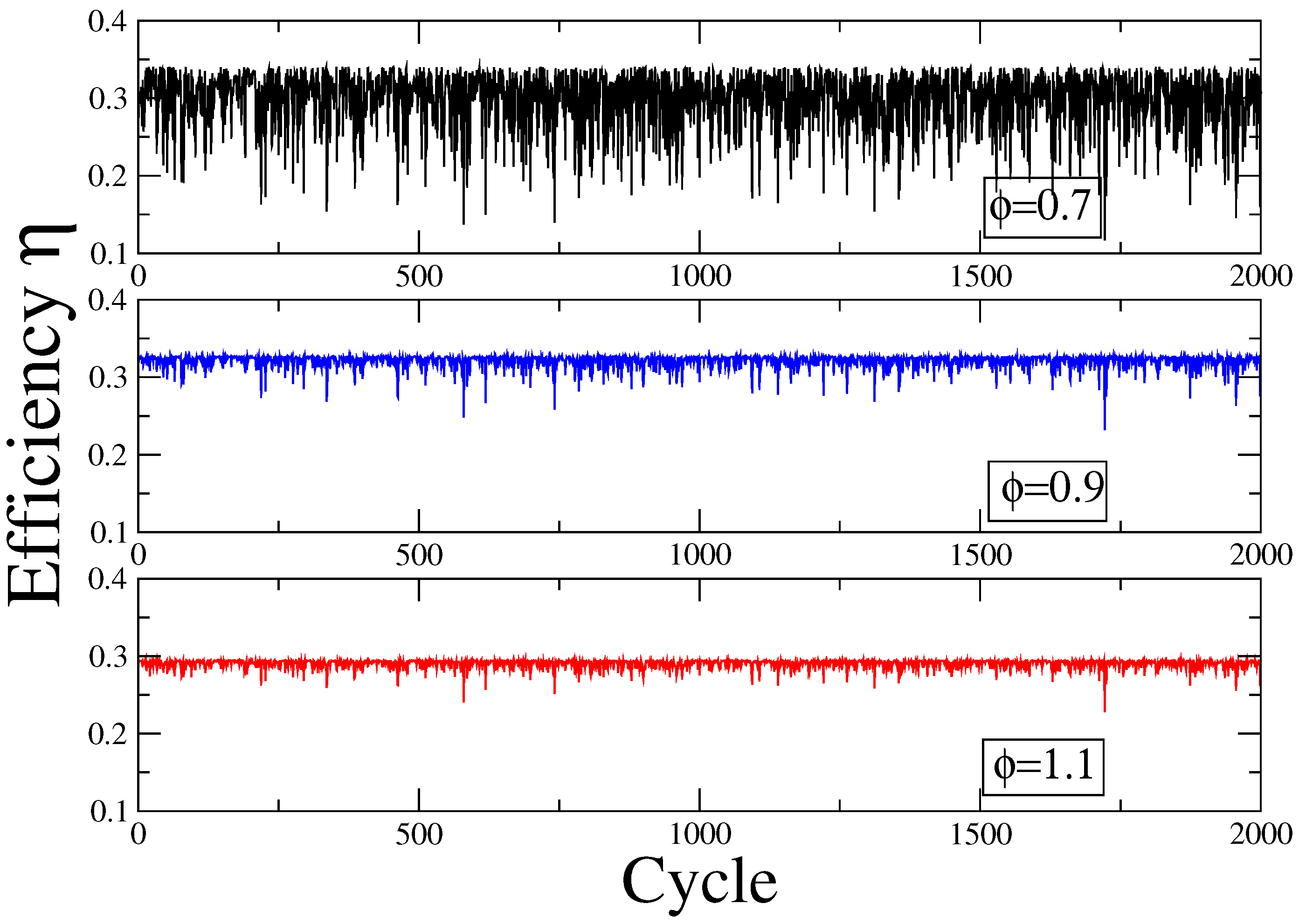
The evolution in time of power and efficiency are presented in Figure 2 and Figure 3, respectively, for the same three values of the fuel ratio. It is worth-mentioning that η is not a thermodynamic efficiency (and thus, a priori is independent of P and $Q_R$), but a fuel conversion efficiency, as defined in [17], $\eta =P/\left({\dot{m}}_f{Q}_{LHV}\right)$, where ${\dot{m}}_f$ is the mass of fuel entering in the cylinder each cycle divided by the cycle duration and $Q_{LHV}$ is the lower calorific value of the fuel. As before, for heat release, we note a noisy behavior both in P and η, with a decreasing amplitude as the fuel ratio increases.

Figure 2. Cycle-to-cycle evolution of the power output, P, for three values of the fuel ratio, $\varphi$.

Figure 2. Cycle-to-cycle evolution of the power output, P, for three values of the fuel ratio, $\varphi$.

Figure 3. Cycle-to-cycle evolution of the fuel conversion efficiency, η, for three values of the fuel ratio, $\varphi$.

Figure 3. Cycle-to-cycle evolution of the fuel conversion efficiency, η, for three values of the fuel ratio, $\varphi$.

In order to analyze and compare these time series of energetic quantities, we calculate some usual statistical parameters: the average value (μ), the standard deviation (STD), the coefficient of variation (COV), the skewness, S, and the kurtosis, K. S is a measure of the lack of symmetry. Negative (positive) values are associated with the existence of left (right) asymmetric tails longer than the right (left) tail. K is a measure of whether the data are peaked ($K>3$) or flat ($K<3$) relative to a normal distribution. 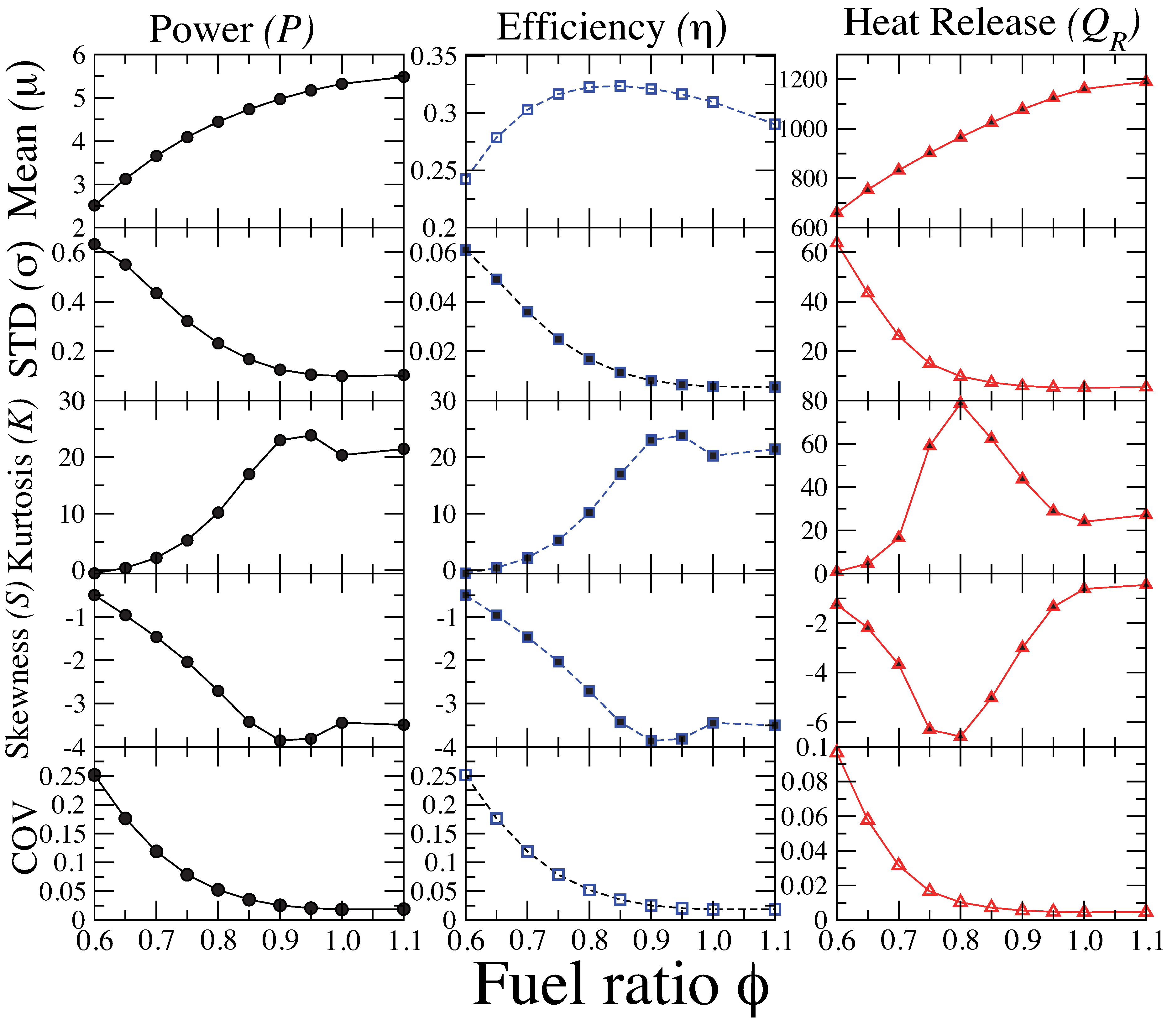In Figure 4, we show the results of the calculations of these statistical parameters for several fuel ratio values. We are not aware of a simultaneous analysis of P, $Q_R$ and η in the literature, neither experimental nor theoretical.

Figure 4. Statistical parameters of the energetic functions considered in terms of the fuel ratio, $\varphi$. Mean value (μ), standard deviation (STD), coefficient of variation (COV), skewness (S) and kurtosis (K) of the power output, efficiency and heat release. In all plots, we have used solid or dashed lines to connect the symbols, as a guide to the eye.

Figure 4. Statistical parameters of the energetic functions considered in terms of the fuel ratio, $\varphi$. Mean value (μ), standard deviation (STD), coefficient of variation (COV), skewness (S) and kurtosis (K) of the power output, efficiency and heat release. In all plots, we have used solid or dashed lines to connect the symbols, as a guide to the eye.

The mean value monotonically increases as the fuel ratio increases for P and $Q_R$, whereas for η, it shows a maximum value around the fuel ratio, $\varphi \approx 0.85$. For the standard deviation, the three quantities show a decreasing behavior as the fuel ratio increases. The coefficient of variation, i.e., the ratio between the dispersion and the mean, also monotonically decreases with the fuel ratio for all the time series, but numerical values are quite different, depending on the considered time series. For power and efficiency, it reaches 0.25 at low fuel ratios. It is 2.5 times larger than for the heat release. The kurtosis, for P and η, increases until reaching a saturation value around $\varphi \approx 0.9$, while the corresponding K for $Q_R$ is characterized by a function with a maximum value located in $\varphi =0.8$. The skewness, S, shows a behavior opposed to that of K for each energetic function. It is almost always negative, indicating (as shown in Figure 1, Figure 2 and Figure 3) that poor combustion events are abundant. For heat release, this is especially intense at fuel ratios between $\varphi =0.7$ and 0.9. For stoichiometric and over stoichiometric mixtures, S for $Q_R$ becomes slightly positive, indicating the existence of high heat release combustion cycles. The same kind of evolution for the statistical parameters of heat release time series was recently found experimentally by Sen et al. [2] for a real Ford 4.6 L V8 spark ignited engine working at 1200 rpm.

Looking Figure 4, it is worth mentioning that the evolution of the statistical properties with the fuel ratio for power output and efficiency is very similar (except for the mean value). As we consider a fuel conversion efficiency, as mentioned above, this means that the denominator in η (a constant multiplied by the mass of fuel inside the cylinder in each cycle), which makes the difference between η and P, does not have a definitive influence on the evolution with the fuel ratio of STD, K and S. In principle, ${\dot{m}}_f$ is fluctuating from one cycle to the following, because of cyclic variability, which slightly changes the thermodynamic conditions and residual gases at exhaust, thus affecting the next intake process. However, our results show that the fluctuations of ${\dot{m}}_f$ do not strongly affect the dependence of STD, K and S with the fuel ratio for η and P. This is because our model considers that the effect of small variations in the fuel mass (due to changes in the thermodynamic state of residual gases) are overshadowed by the main cause of cyclic variability, that is, the turbulent combustion process. With respect to the evolution with $\varphi$ of the mean value of power output and efficiency time series, power output monotonically increases as the mixture in the combustion chamber is more fuel rich, and of course, the same happens for ${\dot{m}}_f$ in such a way that its ratio first increases up to approximately $\varphi =0.8$ or $0.85$ and, afterwards, decreases as the mixture approaches stoichiometry.

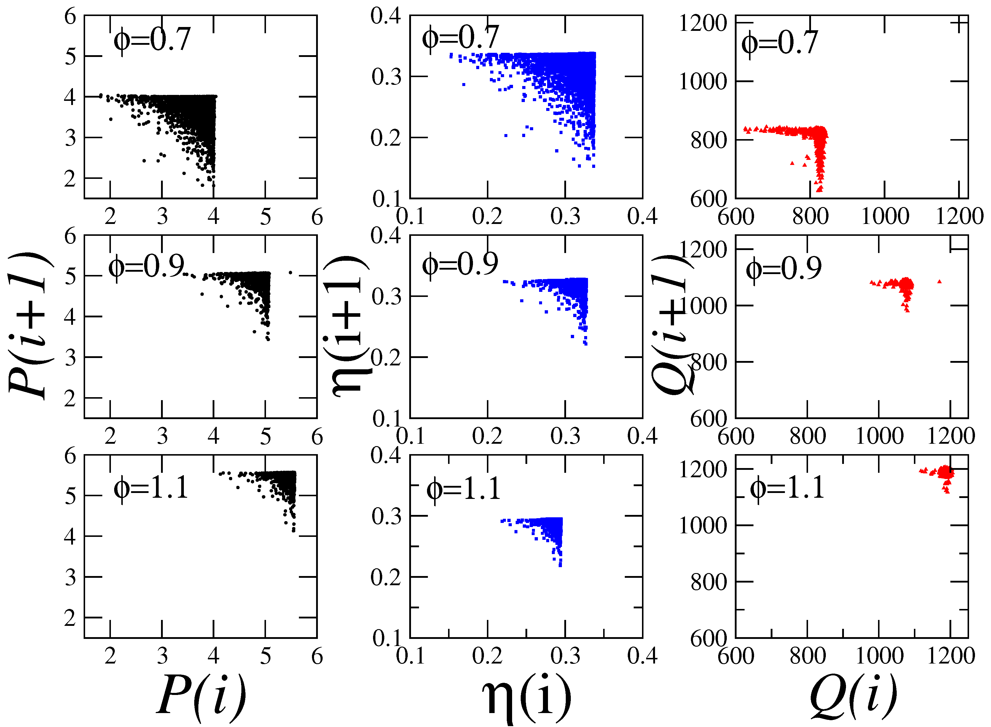
We have plotted in Figure 5 the first return maps of power output, efficiency and heat release. Return maps are a simple testing method to explore one-dimensional dynamics in non-linear time series. They are built by representing the observed variable against itself with a time lag, which in several cases is one. When the plotted map has an unstructured noisy shape, the data likely corresponds to erratic fluctuations with poor memory. A different pattern may constitute a sign of a non-random underlying dynamics. Looking at Figure 5, simulations reveal triangle shaped return plots for power output and efficiency in all the ranges of fuel-air ratios considered. Triangle structured return maps were previously found in experimental results for IMEP and engine torque in no swirl conditions by Wagner et al. [28] and Davis et al. [7]. The evolution of the return maps with the fuel-air ratio for the heat release is evident from Figure 5. For lean mixtures, they have a boomerang shaped structure, which has been found in several experiments and models [1,10,11,29], and they evolve to unstructured noisy spots as fuel-air ratio approaches the stoichiometric value. To go beyond the information given by return maps, we also explore the time organization of P and η by means of the fractal dimension method (FDM). We notice that by means of this type of analysis, we are exploring the presence of correlations that extend over a range of scales, and thus, it is possible to evaluate the presence of correlations beyond small time lags. Briefly, we explain the main steps of FDM [30,31,32]. Given the time series, $x_1,x_2,\dots x_N$, we construct new time series, $x_m^k,$, defined as $x_m,x_{m+k},x_{m+2k},\dots ,x_{(m+\left[\frac{N-k}{k}\right]·k)}$, with $m=1,2,3,\dots ,k$; [ ] denotes Gauss’ notation, that is, the bigger integer, and m and k are integers that indicate the initial time and the interval time, respectively. The length of the curve, $x_m^k$, is defined as:

$$\begin{array}{c}{L}_m\left(k\right)=\frac{1}{k}\left[\left(\sum _{i=1}^{\left[\frac{N-m}{k}\right]}\left|x(m+ik)-x(m+(i-1\left)k\right)\right|\right)\frac{N-1}{\left[\frac{N-m}{k}\right]k}\right]\hfill \end{array}$$

(8)

and the term, $(N-1)/\left[\right(N-m)/k]k$, represents a normalization factor. The length of each sequence, $x_m^k$, is considered to construct the length of the original curve for the time interval, k, $\langle L\left(k\right)\rangle$. Finally, if $\langle L\left(k\right)\rangle \propto k^{-D}$, then the curve is a fractal with dimension, D [30]. It is known that the fractal dimension is related to the spectral exponent, β, by means of $\beta =5-2D$ [30]. We notice that this relationship is valid for $1<D<2$ and $1<\beta <3$, and thus, FDM is not a reliable method for signals with strong anticorrelated behavior, that is, for $-1<\beta <0$. To overcome this problem, we first integrate the original time series prior to applying the standard FDM. In this way, for processes, which can be described as the first derivative of fluctuations with a spectral exponent within the interval, $1<\beta <3$, the relationship between β and D changes to $\beta =3-2D$. A process with positive long range correlations leads to $D<1.5$, whereas for anticorrelated processes, $D>1.5$. The irregular fluctuations with no memory are represented by $D=1.5$. We apply the FDM to the integrated P, η and $Q_R$ sequences for different values of the fuel ratio, $\varphi$.

Figure 5. First return maps of the power output (P), efficiency (η) and heat release ($Q_R$) for three different fuel-air ratios.

Figure 5. First return maps of the power output (P), efficiency (η) and heat release ($Q_R$) for three different fuel-air ratios.

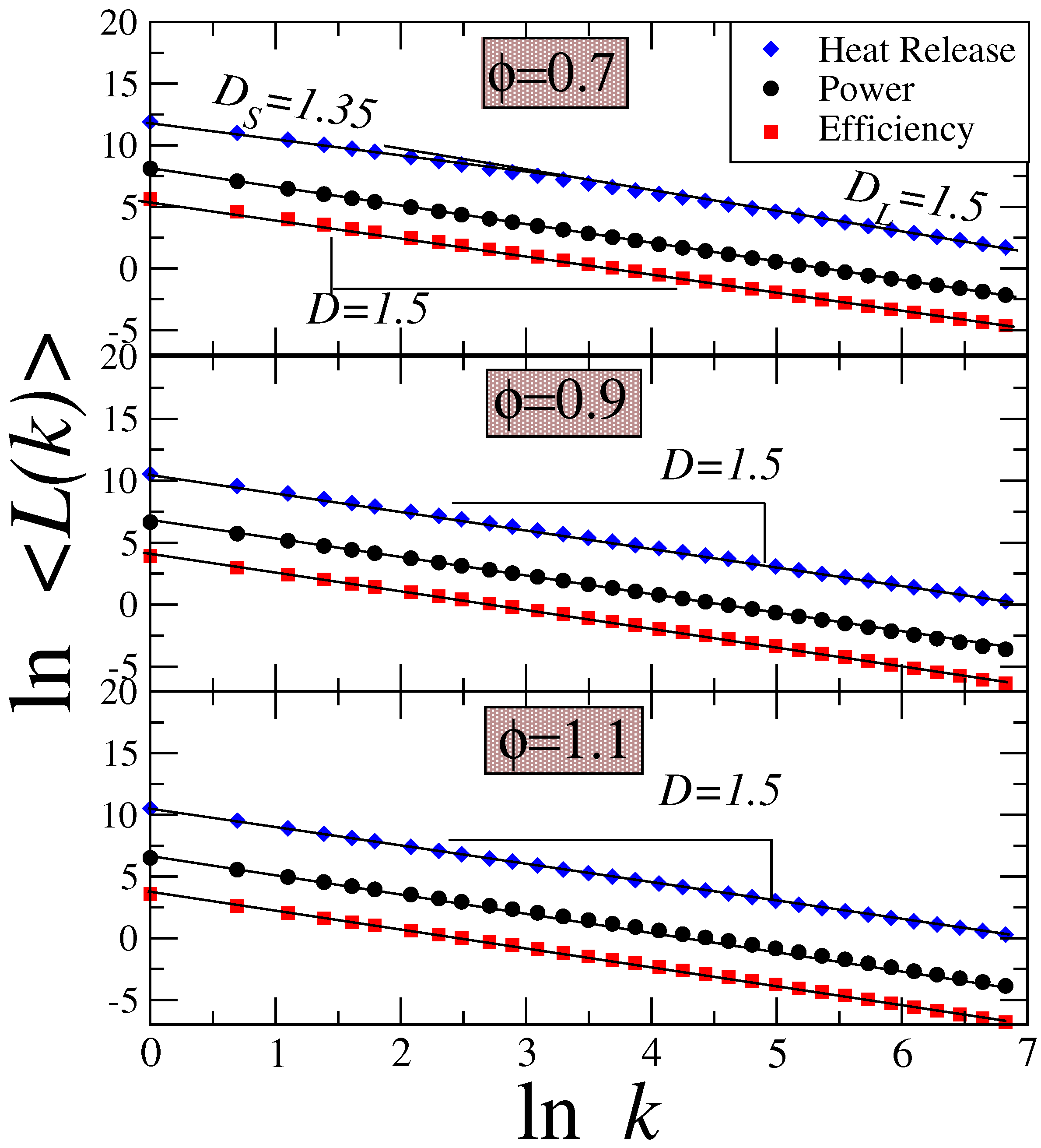
Figure 6 shows the results of the fractal dimension at three different values of $\varphi$. For both performance output functions (η and P), the scaling behavior is described by a single exponent, $D\approx 1.5$, indicating irregular fluctuations. In contrast, for heat release, $Q_R$, the scaling behavior reveal two regimes (for $0.6<\varphi <0.8$); over short scales, the fractal dimension is close to $D_S\approx 1.35$, while for large ones, $D_L\approx 1.5$ [14]. These results indicate that while $Q_R$ exhibits short-term correlations for intermediate values of $\varphi$, both performance output functions are characterized as processes with no memory (white noise fluctuations). A more detailed analysis of the crossover between $D_S$ and $D_L$ observed in $Q_R$ for the interval $0.6<\varphi <0.8$ is described in [14].

Figure 6. Plot of $ln<L\left(k\right)>$ vs. $lnk$ of heat release, $Q_R$ (diamonds), power, P (circles) and efficiency, η (squares), for three of the fuel ratio, $\varphi$. For a fractal signal, it is expected to have $\langle L\left(k\right)\rangle \propto k^{-D}$, where the slope, D, represents the fractal dimension of the set. Here, we see that for P and η, and for any value of $\varphi$, the fractal dimension is $D=1.5$, indicating irregular fluctuations with limited memory. For $Q_R$, a crossover behavior is observed for intermediate values of the fuel ratio.

Figure 6. Plot of $ln<L\left(k\right)>$ vs. $lnk$ of heat release, $Q_R$ (diamonds), power, P (circles) and efficiency, η (squares), for three of the fuel ratio, $\varphi$. For a fractal signal, it is expected to have $\langle L\left(k\right)\rangle \propto k^{-D}$, where the slope, D, represents the fractal dimension of the set. Here, we see that for P and η, and for any value of $\varphi$, the fractal dimension is $D=1.5$, indicating irregular fluctuations with limited memory. For $Q_R$, a crossover behavior is observed for intermediate values of the fuel ratio.

4. Correlations between Heat Release and Performance Output Functions

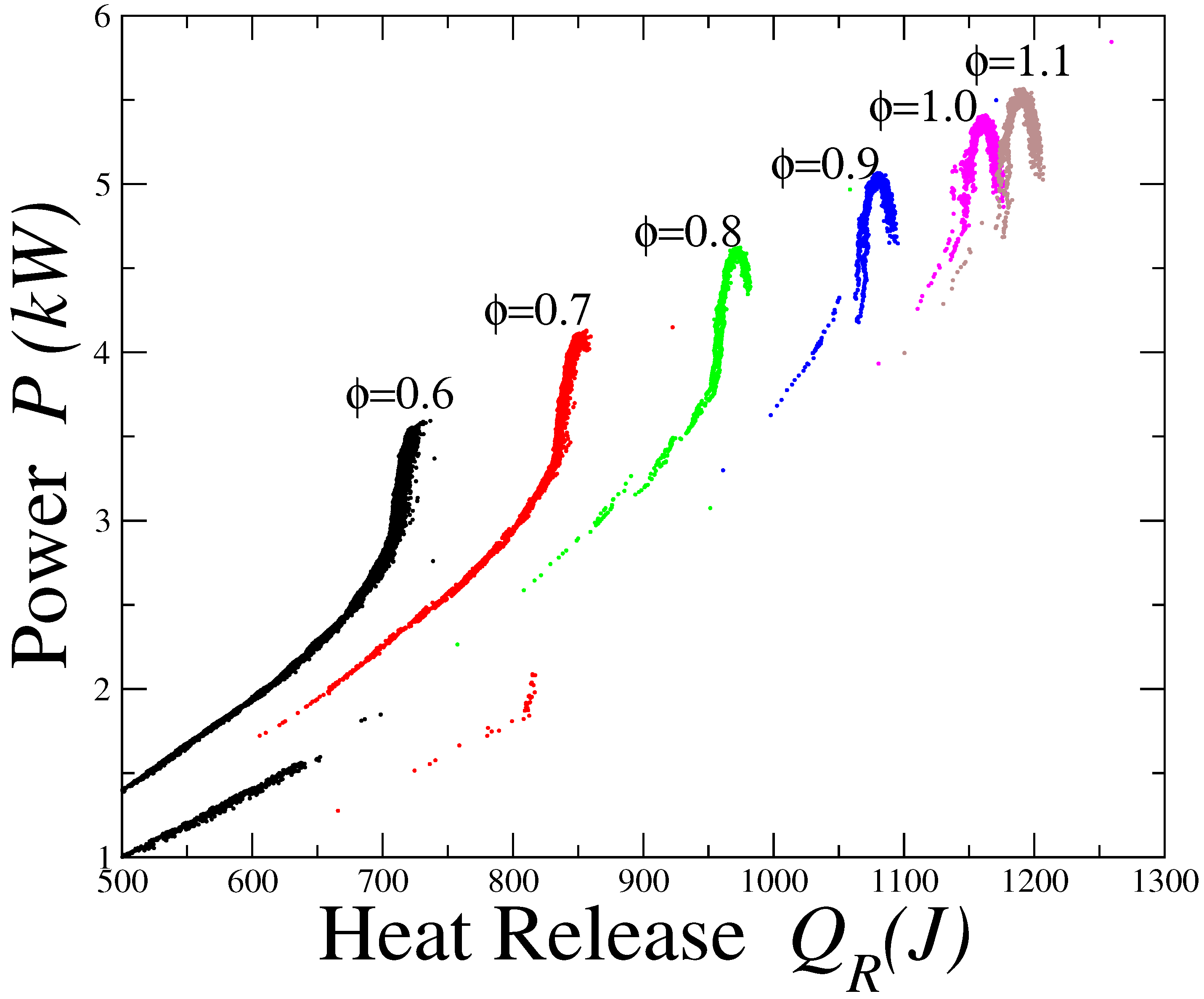
In order to further explore the effect of the fuel ratio on the behavior of the performance output functions, we built the scatter plots as a function of the heat release. Figure 7 and Figure 8 show the scatter plots of P vs. $Q_R$ and η vs. $Q_R$, revealing that the relationship between performance functions and the heat release is far from linear. For lean mixtures (fuel ratios under approximately $0.8$) the highest $Q_R$ leads to the highest power output or efficiency. However, for $\varphi >0.8$, both functions show a maximum and, afterwards, a decreasing evolution. One can roughly identify the values of $Q_R^{*}$, which lead to the maximum value in P and η for each fuel ratio. For $Q_R>Q_R^{*}$, we observe that they lead to values in P smaller than the maximum. The same is observed for the plot, η vs. $Q_R$. In fact, the right wing of the dots distribution observed for $\varphi >0.8$ indicates that even when the heat release is high, the corresponding performance output values are smaller that the maximum, which is reached at a smaller $Q_R$ value.

Figure 7. Scatter plot of P vs. $Q_R$ for several values of the fuel ratio, $\varphi$.

Figure 7. Scatter plot of P vs. $Q_R$ for several values of the fuel ratio, $\varphi$.

Figure 8. Scatter plot of η vs. $Q_R$ for several values of the fuel ratio $\varphi$.

Figure 8. Scatter plot of η vs. $Q_R$ for several values of the fuel ratio $\varphi$.

We notice that for low fuel ratios ($\varphi <0.7$), two clouds of dots (P and η) can be roughly identified for low values of $Q_R$ (Figure 7 and Figure 8). These features result from the fact that $Q_R$ shows a bifurcation-like behavior as the cycle number evolves [31]. However, in real engines, the presence of such bifurcations have not been found [1]. 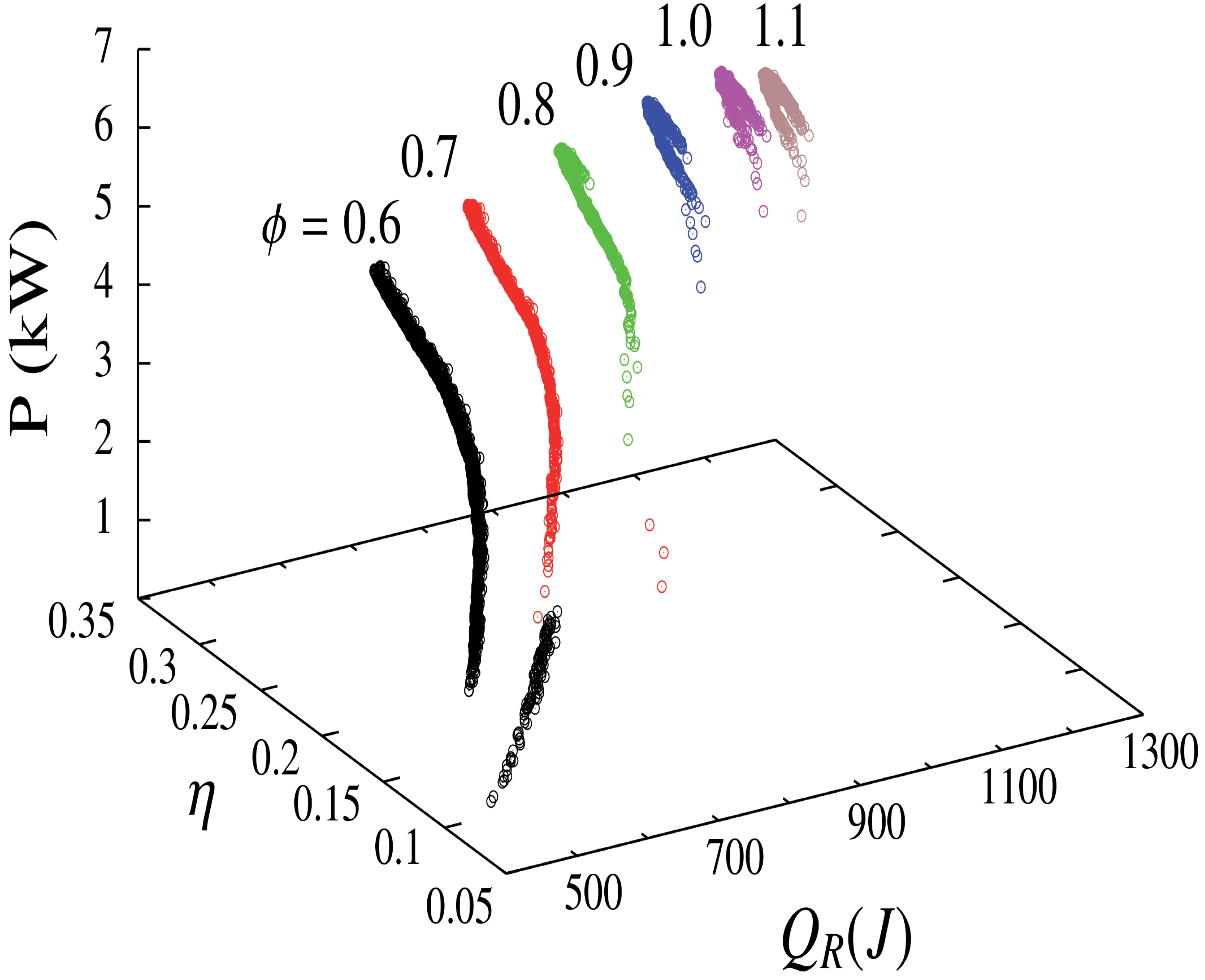In any case, for typical $\varphi$-values of real engines, the zone of these bifurcation-like behaviors are outside the typical optima values of power and efficiency, which usually are within the region that represents a good compromise between both high power and high efficiency [26,33,34]. For completeness, we show in Figure 9 a 3D plot in which the scatter plot of the three considered energetic functions at different fuel ratios are displayed.

Figure 9. Three dimensional scatter plot of $Q_R$, P and η for different mixture compositions.

Figure 9. Three dimensional scatter plot of $Q_R$, P and η for different mixture compositions.

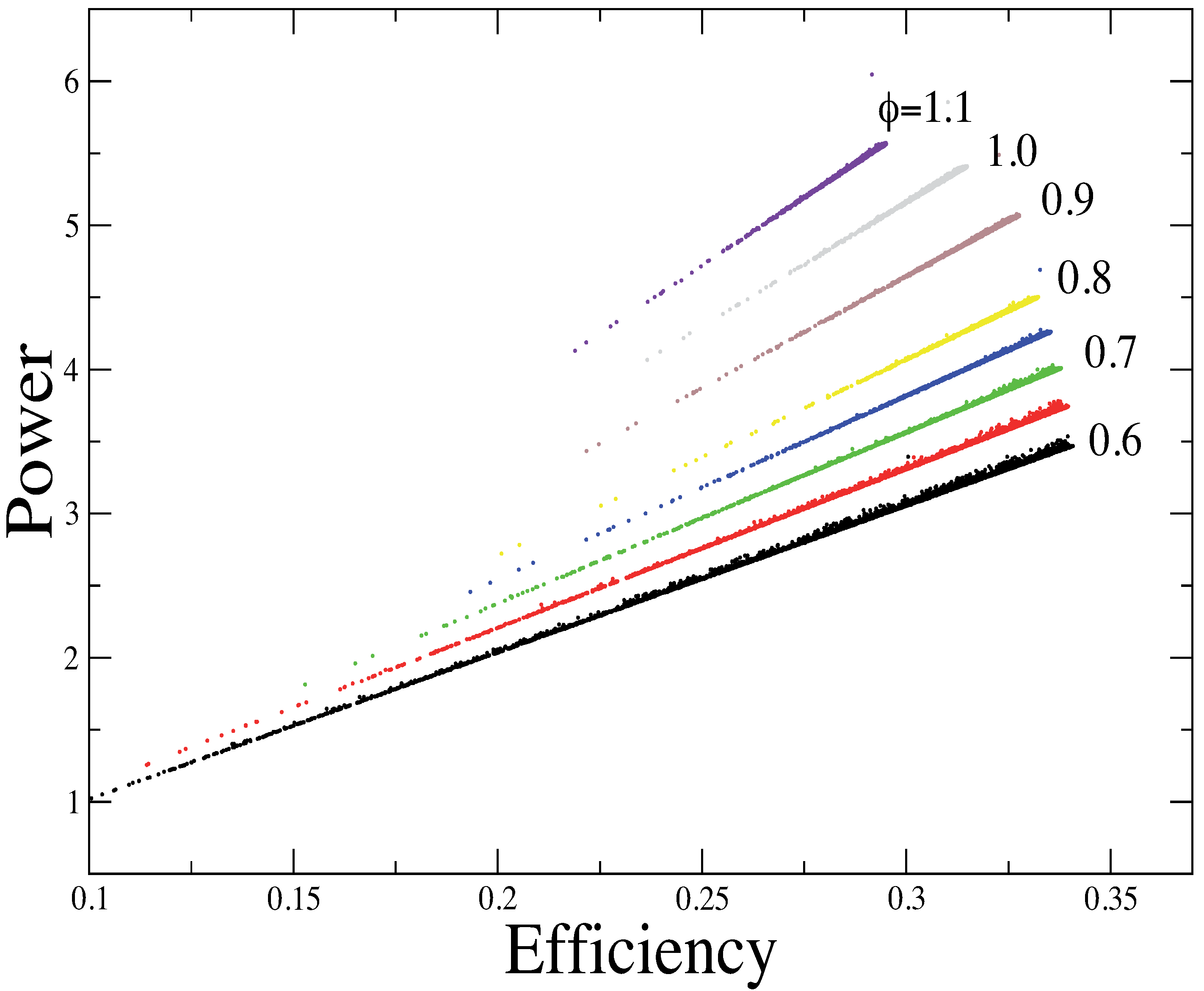
We also explore the behavior of power-efficiency plots to evaluate the effect of stochastic variations together with the fuel ratio on these performance output functions. In Figure 10, we show the plot of P vs. η for several fuel ratio values. It was obtained by considering both P and η as fluctuating functions of the fuel ratio, $\varphi$, taken as a parametric variable. This figure is the probabilistic counterpart of the power-efficiency loop-shaped curves that are usual in thermodynamic optimization for both internal [18,26,31,35,36] and external combustion [37,38,39,40] models. These curves, which constitute a powerful optimization tool in the field of thermodynamic optimization, have the shape of a closed loop (such as the contour of a mussel), with different values for maximum power and maximum efficiency points. They allow us to determine the optimal working region of several energy converters, which is widely considered to be the region between those maximum values [18]. Our results support a clear way to obtain the maximum achievable efficiency for a certain fixed power requirement under noisy conditions. 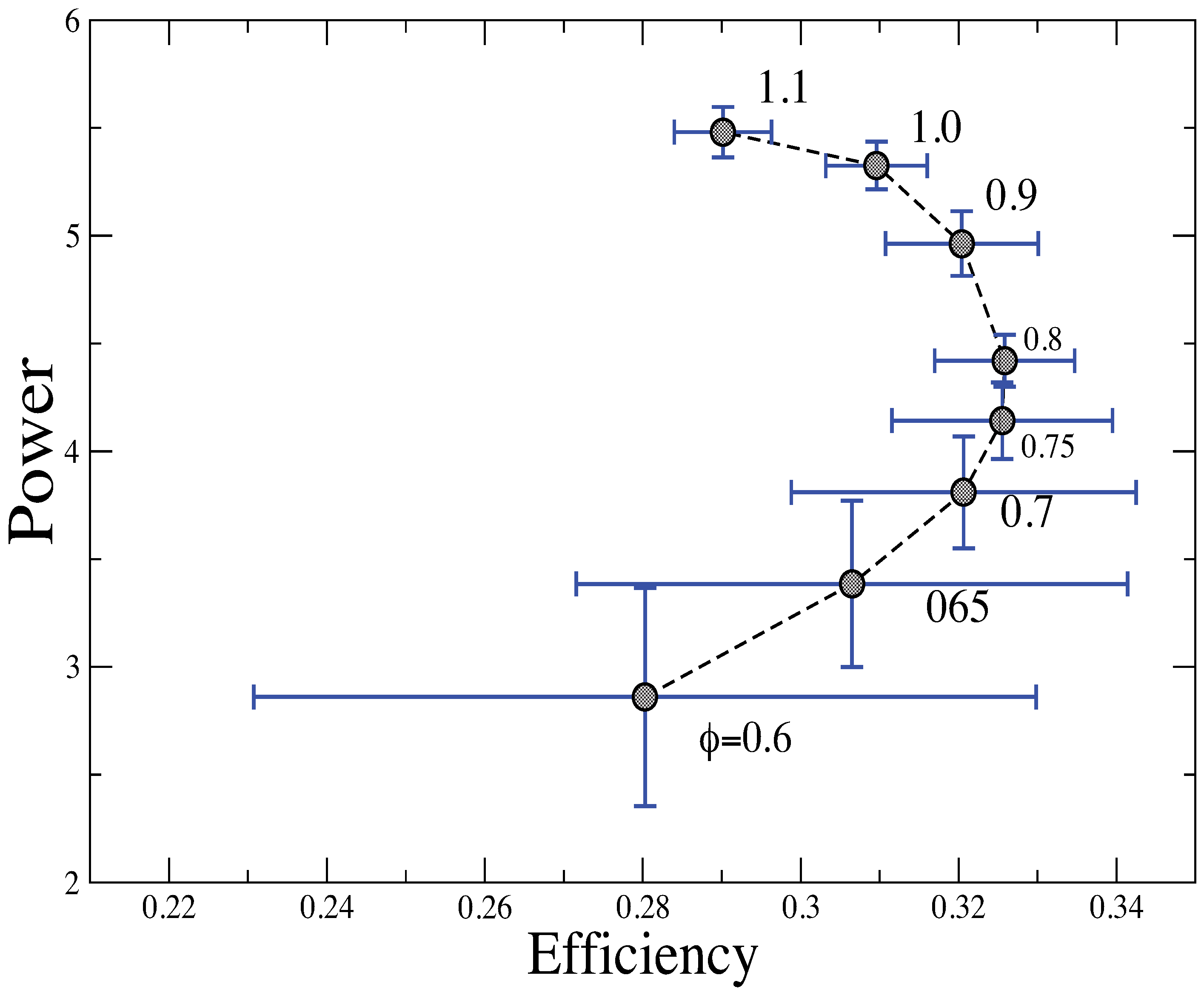As shown in Figure 4, for the lowest equivalence ratios, the distributions for both power and efficiency are quite flat, less peaked than a Gaussian (K is lower than three) and present an asymmetric left tail (S is negative). Opposite, at high equivalence ratios, the observed variations of both power and efficiency are more peaked around the mean than a Gaussian, while the asymmetric left tails still survive. This fact is consistent with the results from the fractal analysis. The influence of the other two statistical parameters, mean and standard deviation, is better reflected in Figure 11, where we show the mean value of $P=P\left(\eta \right)$ that would represent the usual power-efficiency curve together with the standard deviation (as a gross measure of the existence of irreversibilities during the cycle) both of the power output and of the efficiency. The usual (deterministic) power-efficiency curves for several energy converters are loop (closed) curves with different maximum power and maximum efficiency curves. In the limit of no power output and no efficiency, the curves closes in on itself. In our Figure 11, some points of that curve are shown (mean values), but including variability, each mean value has a dispersion in both axes, which is indicated with error bars. This is another interesting way to represent the results of Figure 10. From the figure, the following points are remarkable: (a) the monotonic decrease of the standard deviation as the fuel ratio is close to unity for both power and efficiency; (b) the monotonic increase of the mean value for power accomplished by an efficiency, whose mean value has a maximum at an intermediate fuel ratio. A clear consequence is the observed loop-shaped power versus efficiency plots, which clearly reflect, in a probabilistic manner, the well-known features of the non-coincident maximum power and maximum efficiency points. Furthermore, as usual for stationary engines, the optimal values for power and efficiency are in between these points.

Figure 10. Scatter plot of power vs. efficiency for several values of the fuel ratio, $\varphi$.

Figure 10. Scatter plot of power vs. efficiency for several values of the fuel ratio, $\varphi$.

Figure 11. Power-efficiency plots showing the mean value and the standard-deviation in both axis for different values of $\varphi$.

Figure 11. Power-efficiency plots showing the mean value and the standard-deviation in both axis for different values of $\varphi$.

5. Summary and Conclusions

We have presented a probabilistic and quasi-dimensional simulation model incorporating the main chemical and physical ingredients affecting the turbulent combustion process in a spark-ignition engine. The cycle-by-cycle variations in energetic indicators are analyzed by assuming a fluctuating character of the characteristic length of the unburned eddies entrained within the flame front.

The consequences on heat release, power output and efficiency are studied for fuel-air equivalence ratios ranging from lean mixtures to over stoichiometric conditions. Well-known unified behaviors of these magnitudes in the finite-time-thermodynamics framework are correctly reproduced by considering the corresponding mean values, while other statistical parameters, such as the standard deviation, the skewness and the kurtosis, allow for a clearer interpretation of subtle features. Particularly, the evolution with the fuel ratio of the statistical parameters characterizing the time series of heat release (the most usual energetic variable measured in cyclic variability experiments) is in good accordance with experimental results [2]. Furthermore, the return maps obtained for the three variables considered are consistent with those found in previous experimental and theoretical models. Triangle shaped return maps are observed for power output and efficiency with a light evolution with the fuel-air ratio. Nevertheless, heat release shows boomerang shaped first return maps at lean conditions that transforms into noisy unstructured spots as stoichiometric conditions are reached. By means of the FDM method, we have shown that heat release displays short-term correlations at low values of fuel ratios ($\varphi \simeq 0.7$), whereas efficiency and power output always show irregular variations with poor memory.

Scatter plots of power output and fuel conversion efficiency as functions of heat release show that the relationships are not linear. For intermediate and near stoichiometric fuel ratios, both power and efficiency display a convex behavior with maximum values in terms of heat release, i.e., during the fluctuating evolution of heat release, the highest value does not guarantee a maximum power output or efficiency. We have also computed probabilistic power vs. efficiency plots by eliminating the fuel ratio considered as a parametric variable. As fuel ratio tends to unity, dispersion (such as a gross measure of irreversibilities coming from turbulent combustion, turbulence in the intake and exhaust processes and other physical phenomena provoking cyclic variability) in both axes diminishes. The mean value of efficiency and power for each fuel ratio recovers the well-known power vs. efficiency curves widely used in thermodynamic optimization.

The energetic analysis presented here is consistent with the typical energetic results of steady state studies represented by average values only. In fact, Figure 11 shows how low values of fuel ratio ($\varphi <0.7$) are concomitant with large fluctuations of power and efficiency. This result is in agreement with previous fractal and multifractal studies of the same system. On the other hand, for large values of the fuel ratio ($\varphi >0.9$), we observe regimes of performance with low efficiency and high power characterized by small fluctuations. In between these two regimes, the maximum efficiency point is located. We have checked that all these conclusions are independent of the particular parameters of the engine for which the numerical results have been shown. We finish by recalling attention to the importance of quasi-dimensional models in order to get performance data (with low computational cost), which can be used to elaborate thermodynamic models that, in turn, offer a reliable comparison with the observed indicators. As has been investigated in the context of CFDmodels of in-cylinder turbulence [41], large-scale turbulent eddies could persist from cycle-to-cycle and, so, could be temporally correlated. The consideration of these correlations could lead to a more precise simulation of certain patterns of cycle-to-cycle fluctuations that standard quasi-dimensional models cannot predict. One of the critical points when developing this kind of simulation model is the flame propagation sub-model, because traditional flame speed correlations fail as the lean flammability limit is approached [42,43]. In these conditions, the assumption of a smooth, spherically progressing flame front should be revised. This probably provokes the combustion response to small changes in the fuel-air ratio much more non-linearly than at higher fuel-air ratios. The investigation of cycle-to-cycle correlations in turbulence and the effects of criticality-type flame propagation processes are tasks for future studies.