Article

A Thermodynamical Selection-Based Discrete Differential Evolution for the 0-1 Knapsack Problem

1
Institute of Medical Informatics and Engineering, School of Science, JiangXi University of Science and Technology, Ganzhou 341000, China
2
College of Computer Science and Technology, Zhejiang University, Hangzhou 310027, China
3
School of Information Engineering, Shijiazhuang University of Economics, Shijiazhuang 050031, China
4
State Key Laboratory of Software Engineering, Wuhan University, Wuhan 430072, China
*
Author to whom correspondence should be addressed.
Entropy 2014, 16(12), 6263-6285; https://doi.org/10.3390/e16126263
Submission received: 2 October 2014 / Revised: 8 November 2014 / Accepted: 21 November 2014 / Published: 28 November 2014
(This article belongs to the Special Issue Entropy in Bioinspired Intelligence)

Abstract

:
Many problems in business and engineering can be modeled as 0-1 knapsack problems. However, the 0-1 knapsack problem is one of the classical NP-hard problems. Therefore, it is valuable to develop effective and efficient algorithms for solving 0-1 knapsack problems. Aiming at the drawbacks of the selection operator in the traditional differential evolution (DE), we present a novel discrete differential evolution (TDDE) for solving 0-1 knapsack problem. In TDDE, an enhanced selection operator inspired by the principle of the minimal free energy in thermodynamics is employed, trying to balance the conflict between the selective pressure and the diversity of population to some degree. An experimental study is conducted on twenty 0-1 knapsack test instances. The comparison results show that TDDE can gain competitive performance on the majority of the test instances.

1. Introduction

Many problems in business and engineering can be modeled as 0-1 knapsack problems [1,2], such as project selection, resource distribution and investment decision-making problems. In the 0-1 knapsack problem, given D items, each of them has a weight Wj and a profit Pj [3]. The aim is to choose a subset from the D items to maximize the overall profit without exceeding the weight capacity C of the knapsack [4]. Mathematically, the 0-1 knapsack problem can be formulated as follows:
Max f ( X ) = j = 1 D P j X j s . t . { j = 1 D W j X j C X j { 0 , 1 } , j = 1 , , D
where Xj is a binary decision variable, which indicates that item j is contained in the knapsack or not. Wj and Pj are the weight and profit of item j, respectively. C is the maximum weight capacity of the knapsack, and D is the number of items. However, the 0-1 knapsack problem is one of the classical NP-hard problems [46], which means that no exact algorithms are known to obtain the optimum solutions for this problem in polynomial computation time. Therefore, it is of significance both in theory and in engineering applications to develop effective and efficient algorithms for the 0-1 knapsack problems.
Evolutionary algorithms (EAs) are effective heuristic algorithms for solving global optimization problems [711]. Moreover, many kinds of evolutionary algorithms have been successfully applied to solve the 0-1 knapsack problem in the past few decades. Shi [12] proposed an improved ant colony algorithm for solving 0-1 knapsack problems. In the improved ant colony algorithm, a novel pheromone updating strategy is designed according to the characteristics of the 0-1 knapsack problems. Neoh et al. [13] introduced a layered encoding cascade evolutionary approach (LGAPSO) to solve 0-1 knapsack problems. In LGAPSO, genetic algorithm (GA) and particle swarm optimization (PSO) are utilized for searching the global optimum. Shang et al. [14] proposed a quantum immune clonal selection algorithm (QICSA) for solving the multi-objective 0-1 knapsack problem. QICSA uses a string of qubits to represent the solutions and employs a chaotic search strategy to generate a new antibody. Layeb [15] introduced a novel quantum-inspired cuckoo search for 0-1 knapsack problems. A quantum-inspired tabu search algorithm (QTS) is proposed by Chiu et al. [16] for solving 0-1 knapsack problems. The experimental results indicate that QTS performs much better than the other heuristic algorithms on 0-1 knapsack problems. Zou et al. [4] presented a novel harmony search algorithm (NGHS) to solve 0-1 knapsack problems. In NGHS, a position updating scheme and a genetic mutation operator with a small probability are utilized to improve the performance of the traditional harmony search algorithm. A modified binary particle swarm optimization algorithm is proposed by Bansal and Deep [5] for 0-1 knapsack problems. Sabet et al. [17] presented a binary version of the artificial bee colony algorithm to solve the 0-1 knapsack problem. In the proposed binary artificial bee colony algorithm, a hybrid probabilistic mutation scheme is utilized for searching the neighborhood of food sources. Gherboudj et al. [18] introduced a discrete binary version of the cuckoo search algorithm for solving 0-1 knapsack problems. In the literature [19], a hybrid quantum inspired harmony search algorithm is proposed by Layeb for solving 0-1 knapsack problems. Lu and Yu [20] introduced a quantum multi-objective evolutionary algorithm with an adaptive population (APMQEA) to solve multi-objective 0-1 knapsack problems. In the search process, APMQEA fixes the number of Q-bit individuals assigned to each objective solution, while it adaptively updates its population size according to the number of found non-dominated solutions. Deng et al. [21] introduced a binary encoding differential evolution for solving 0-1 knapsack problems. Truong et al. [6] presented a chemical reaction optimization with a greedy strategy algorithm (CROG) for solving 0-1 knapsack problems. The experimental results reveal that CROG is a competitive algorithm for solving 0-1 knapsack problems. In the literature [22], an amoeboid organism algorithm is proposed by Zhang et al. to solve 0-1 knapsack problems.
Among the evolutionary algorithms, differential evolution, proposed by Storn and Price in 1997 [23], is a simple, yet effective, global optimization algorithm. According to frequently reported theoretical and experimental studies, differential evolution (DE) has demonstrated better performance than many other evolutionary algorithms in terms of both convergence speed and solution quality over several benchmark functions and real-life problems [2426]. Due to its effectiveness, as well as global search capability, DE has attracted many researchers’ interests since its introduction. Thus, it has become a research focus of evolutionary computation in recent years [25,26].
However, DE adopts a one-to-one greedy selection operator between each pair of the target vector and its corresponding trial vector, which exhibits weak selective pressure due to unbiased selection of parents or target vectors [25,26]. Furthermore, this weakness may lead to inefficient exploitation when relying on differential mutation, especially on the rotated optimization problems [26]. A straightforward way to alleviate this shortcoming may be to enhance the selection operator to improve the selective pressure. In fact, such mechanism indeed can promote the exploitation capacity of DE. However, high selective pressure may often lead to rapid loss of population diversity and, thus, increase the probability of being trapped in local minima. Therefore, increasing the selective pressure in DE is often in conflict with promoting the population diversity, which indicates that a feasible solution to alleviate this weakness of DE cannot merely improve one of the selective pressures or the population diversity [25,26].
Nevertheless, to the best of our knowledge, it is one of the most challenging issues of DE to keep a balance between the selective pressure and the diversity of population. Thus, in this paper, we propose a promising discrete DE (TDDE) using an enhanced selection scheme (MFES) inspired by the principle of the minimal free energy in thermodynamics, trying to palliate the conflict between the selective pressure and the population diversity to some degree. Further, the proposed algorithm is applied to the 0-1 knapsack problems.
The rest of the paper is organized as follows. The conventional DE and discrete DE are introduced in Section 2. Section 3 presents the improved selection operator of DE inspired by the principle of the minimal free energy in thermodynamics, which is useful for elaborating the implementation of the proposed algorithm, TDDE, in Section 4. Numerical experiments are presented in Section 5 for the comparison and analysis. Finally, Section 6 concludes this paper.

2. Differential Evolution

Like other evolutionary algorithms (EAs), DE is a simple, yet efficient, stochastic optimization technique, which has a simple structure, only consisting of easy operators, namely, mutation, crossover and selection operators [23,27,28]. Therefore, it is easy to understand and implement. However, it exhibits better search performance than many other evolutionary algorithms in terms of convergence speed and solution accuracy in many practical applications [26,29,30].
Because the 0-1 knapsack problem is a maximization optimization problem, we only consider maximization problems in this study. We assume that the objective function to be maximized by DE is Max f(X), X = [X1, X2, …, XD], and the search space is:
Ω = j = 1 D [ L o j , U p j ]
where D is the dimensionality of the problem to be optimized and Loj and Upj are the lower and upper boundaries of the search space. In the search process, DE starts with an initial population P ( t ) = { X i t } randomly sampled from the search space, where X i t = [ X i , 1 t , X i , 2 t , , X i , D t ] , i = 1 , 2 , , N P ; NP is the population size and t is the generation. After initialization, DE executes its mutation, crossover and selection operators repeatedly to move its population toward the global optimum until the termination condition is satisfied [31]. Next, we will elaborate the evolutionary operators of DE as follows.

2.1. Mutation Operator

In the mutation operator, DE generates a mutant vector V i t by a preset mutation strategy for each individual X i t, called a target vector, in the current population [26,30]. There are many mutation strategies used in the DE implementations [26,32], such as DE/rand/1, DE/best/1, DE/rand-to-best/1, DE/best/2/and DE/rand/2. The most frequently used one is DE/rand/1, which is described as follows [23,26].
V i t = X r 1 t + F × ( X r 2 t X r 3 t )
where the indices r1, r2, r3 are mutually exclusive integers randomly selected from the set {1, 2, …, NP} \ {i}. F is a scaling factor, which scales the difference vector X r 2 t X r 3 t.

2.2. Crossover Operator

After mutation, a crossover operator is utilized for each pair of target vector X i t and its corresponding mutant vector V i t to create a trial vector U i t [26,29,33]. Binomial and exponential crossovers are two commonly used crossover schemes in the current popular DE. The binomial crossover is expressed in the following form [23,26].
U i , j t = { V i , j t , if rand ( 0 , 1 ) < CR or j = = jrand X i , j t , otherwise
where rand(0,1) is a uniformly distributed random number within the range [0, 1], which is produced for each j, and CR ∈ [0, 1] is called a crossover probability, controlling the number of components duplicated from the mutant vector V i t j r a n d is a random integer selected from the range [1, D], which ensures that the trial vector U i t differs from its corresponding target vector X i t by at least one dimension.

2.3. Selection Operator

Generally, if the values of some parameters of the trial vector U i t violate the predefined corresponding upper and lower boundary constraints, we randomly and uniformly reset the violating components within the preset range [27]. Then, the objective function values of all of the trial vectors are evaluated. Next, DE executes the selection process in order to select the better individuals to enter the next generation. For maximization problems, the selection operator can be formulated as follows [23,26].
X i t + 1 = { U i t , if f ( U i t ) f ( X i t ) X i t , otherwise
where f ( X i t ) and f ( U i t ) are the objective function values of the target vector X i t and its corresponding trial vector U i t, respectively.

2.4. Discrete Mutation Operator

As is known, the individuals of the traditional DE are represented as real-value vectors. Therefore, the traditional DE cannot directly handle the combinatorial optimization problems. To this end, many researchers have improved the mutation operators of the traditional DE for solving combinatorial optimization problems, presenting discreet DE, among which novel hybrid discrete differential evolution (W_DDE) is proposed by Wang [34]. The enhanced mutation operator of W_DDE is represented as follows [34].
V i , j t = X r 1 , j t F ( X r 2 , j t X r 3 , j t )
where the indices r1, r2, r3 are the same as those in Formula (3). The above formula includes two parts. The first part is,
Δ i , j t = F ( X r 2 , j t X r 3 , j t ) Δ i , j t = { X r 2 , j t X r 3 , j t , if rand ( 0 , 1 ) < F 0 , otherwise
and the second part is,
V i , j t = X r 1 , j t Δ i , j t V i , j t = mod ( ( X r 1 , j t + Δ i , j t + D ) , D )
where mod is the modulus function.

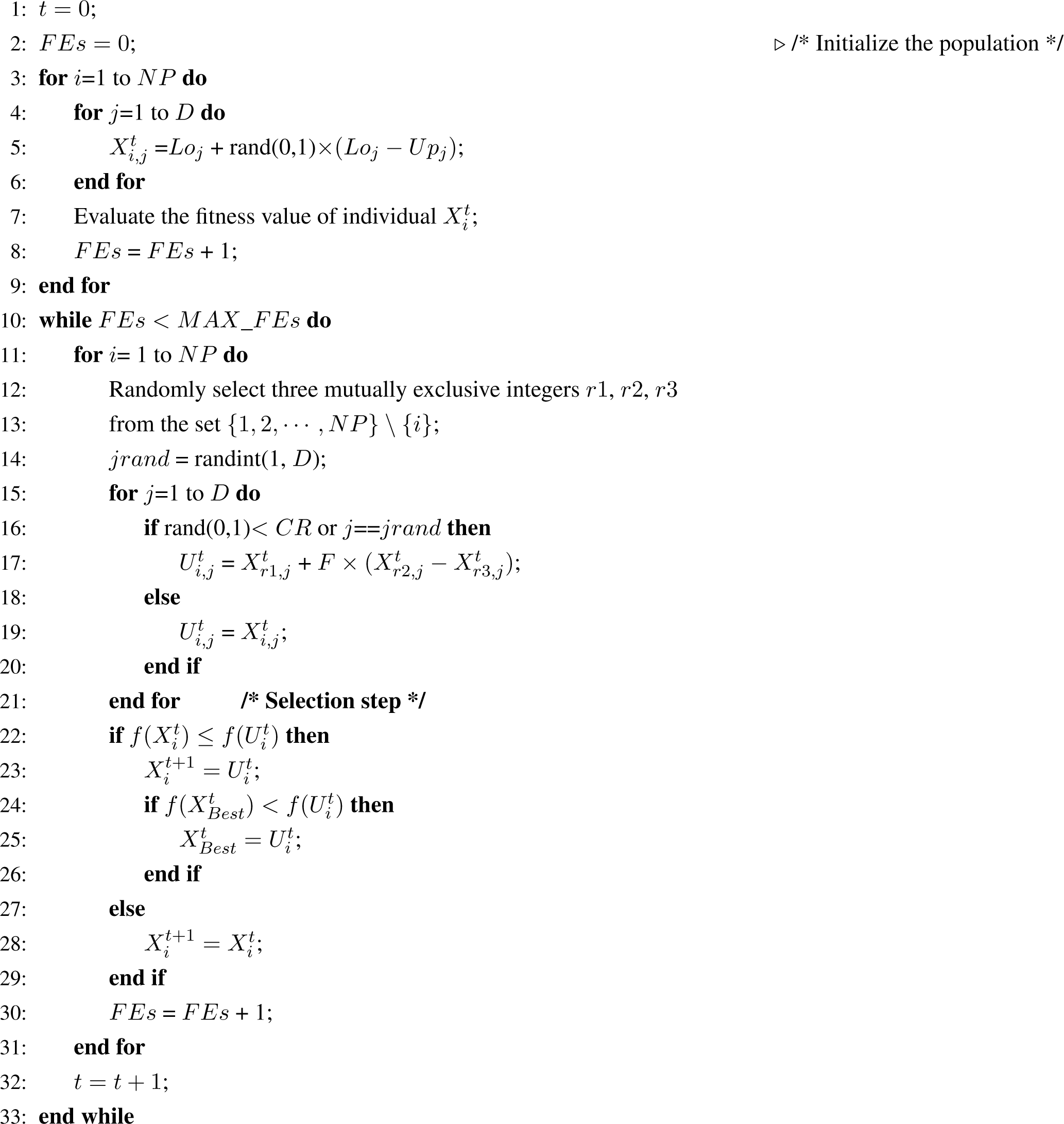
2.5. Algorithmic Description of DE

Based on the above detailed descriptions of the mutation, crossover and selection operators of DE, the algorithmic description of DE with the DE/rand/1/bin strategy is summarized in Algorithm 1, where FEs is the number of fitness evaluations and Max_FEs is the maximum number of evaluations.
Algorithm 1. Differential Evolution (DE) Algorithm.
Entropy 16 06263f1

3. Proposed Selection Operator for DE

3.1. Motivations

As is known, both selective pressure and population diversity are significant for EAs [3538]. However, in the traditional DE, a one-to-one competition mechanism is utilized as the selection operation between each pair of the target vector and its corresponding trial vector, which may induce weak selective pressure owing to its unbiased selection of parents or target vectors [26]. In addition, the traditional DE selects individuals for the next generation merely based on the fitness values [26]. As a result, the selection operator may cause deficient exploitation when depending on differential mutation, especially on the rotated optimization problems [25,26]. In order to enhance the selection operator of the traditional DE, in this section, we propose an improved selection operator, MFES, which is inspired by the principle of the minimal free energy in thermodynamics, trying to palliate the conflict between the selective pressure and the population diversity to some degree. The principle of the minimal free energy refers to [3942], in the annealing process, a metal, beginning with high temperature and chaotic state, is gradually cooled, so that the system at any temperature approximately reaches thermodynamic equilibrium. This cooling process can be regarded as an adaptation procedure to reach the stability of the final crystalline solid. In addition, any change from non-equilibrium to equilibrium of the system at each temperature abides by the principle of the minimal free energy. This means the system will change spontaneously to reach a lower total free energy and the system achieves equilibrium when its free energy seeks a minimum [4042]. The free energy F is defined by:
F = E T H
where E is the mean energy of the system, H is the entropy and T is the temperature. According to the principle of the minimal free energy, we can realize that any change from non-equilibrium to equilibrium of the system can be regarded as a consequence of the competition between the mean energy and the entropy, and the temperature T determines their relative weights in the competition [39,41,42]. Accordingly, the competition between the mean energy and the entropy in the annealing process is the same as the competition between the selective pressure and the population diversity of DE during the evolution process. Therefore, we can alleviate the conflict between the selective pressure and the diversity of population according to the principle of the minimal free energy.
Inspired by [4143], in the improved selection scheme, we firstly map the selective pressure and the population diversity of DE into the mean energy E and the entropy H in the principle of the minimal free energy, respectively. Then, the criterion of the proposed selection scheme is converted to the minimal free energy, which means that we select individuals for the next generation from the parent, and the offspring population should satisfy the principle of the minimal free energy. More specifically, in the selection process, we start with computing the free energy of each individual in the parent and offspring population; then, the top NP individuals with minimal free energy are selected for the next generation. Therefore, the selected individuals for the next generation satisfying the principle of the minimal free energy indicate that the improved selection scheme maintains the fitness value of the next generation population as well as possible, while preserving the most possible diversity. Thus, the proposed selection scheme simultaneously considers the factors of solution quality and the diversity of the population.

3.2. Energy

As discussed above, we should map the selective pressure of DE into the mean energy E in the principle of the minimal free energy. In general, the higher selective pressure may directly lead to the better individuals selected for the next generation. Therefore, we can measure the selective pressure by the fitness values of the selected individuals [41]. The energy E of each individual is mapped into the normalized fitness value of the corresponding individual. Mathematically, the energy E ( X r t ) of any individual X r t is defined by:
E ( X r t ) = bl t ( f ( X r t ) ) bl t bu t = bl t f ( X r t ) bl t bu t
Because the 0-1 knapsack problem is a maximization optimization problem, whereas the criterion of the proposed selection scheme is the minimal free energy, the energy E ( X r t ) of any individual X r t is defined by the normalized f ( X r t ), where f ( X r t ) is the objective function value of individual X r t, the characteristic of whose fitness value is that the larger fitness value reflects the individual better. blt, but are the lower and upper boundaries of the fitness values of the parent population Pt and offspring population Ot at generation t, respectively. blt, but are defined by:
bl t = min { f ( X r t ) | X r t P t O t }
bu t = max { f ( X r t ) | X r t P t O t }

3.3. Entropy

As pointed out in Section 3.1, we should also map the population diversity of DE into the entropy H in the principle of the minimal free energy. Generally, the distribution of the individuals can directly reflect the population diversity [41]. Thus, we divide the fitness values of the individuals into K ranks. Then, we count the number of individuals in each rank to measure the population diversity. The i-th rank β i t is defined by:
β i t = ( bl t + a i 1 1 a K 1 1 ( bu t bl t ) , bl t + a i 1 a K 1 1 ( bu t bl t ) ] [ bl t , bu t ]
where i = 0, 1, …, K − 1; a is a factor related to the width of each rank, set to two in the proposed approach, and K ≥ 2 is the number of ranks. For any individual X r t, if E ( X r t ) β i t, this means that X r t is located in the rank β i t. For any individual X r t located in the rank β i t, assuming the number of individuals within the rank β i t is ni, the entropy H of individual X r t is defined as follows:
H ( X r t ) = log K ( n i N P + M )
where NP is the number of individuals in the parent population Pt and M is the size of the offspring population Ot at generation t. It is known that the population diversity is better while the value of log K ( n i N P + M ) is larger [41]. However, the criterion of the proposed selection scheme is the minimal free energy. Thus, the entropy H of individual X r t is defined as log K ( n i N P + M ). Based on the definitions of the energy E and the entropy H above, for any individual X r t, its free energy is calculated as:
F ( X r t ) = E ( X r t ) T H ( X r t ) = bl t + f ( X r t ) bl t bu t + T log K ( n i N P + M )
where T is the temperature, which is gradually cooled as the evolutionary process proceeds.

3.4. Description of Thermodynamical Selection Operator for DE

Based on the notations and terminologies of the MFES selection scheme in DE, the procedure of MFES in DE is described as follows. Firstly, a temporary population P t + 1 is created by combining the parent population Pt with the offspring population Ot at generation t. Then, the free energy of each individual in the temporary population P t + 1 is calculated according to Equation (15). After that, the top M individuals with maximal free energy are chosen to delete from the temporary population P t + 1. Subsequently, all of the remaining individuals in the temporary population P t + 1 are selected for the next generation population Pt+1. The detailed procedure of the MFES selection scheme in DE is shown in Algorithm 2.
Algorithm 2. MFES selection scheme for differential evolution.
Input: Temperature T, the parent population Pt and the offspring population Ot;
Output: The next generation population Pt+1;
1: Combine the parent population Pt with the offspring population Ot to constitute a temporary population P t + 1;
2: Calculate the free energy of each individual in the temporary population P t + 1 according to Equation (15);
3: Choose the top M individuals with maximal free energy;
4: Remove the chosen M individuals from P t + 1;
5: Create the next generation population Pt+1 by the remaining individuals in P t + 1.

4. Proposed TDDE

Based on the description of the thermodynamical selection operator for DE, in this section, we propose an enhanced discrete DE for the 0-1 Knapsack problem, which selects the individuals for the next generation using the proposed thermodynamical selection operator.

4.1. Population Initialization

In the population initialization process, NP 0-1 vectors with D dimensions are randomly generated. For the i-th individual X r t, it is initialized by:
X i , j t = { 1 , if rand ( 0 , 1 ) < 0.5 0 , otherwise
where rand(0,1) is a uniformly distributed random number within the range [0, 1], which is produced for each j; j = 1, 2,…, D; i = 1, 2,…, NP ; NP is the population size, and D is the number of items.

4.2. Discrete Mutation Operator

Inspired by [34], we design a 0-1 discreet mutation operator in TDDE as follows:
V i , j t = X r 1 , j t F ( X r 2 , j t X r 3 , j t )
where the indices r1, r2, r3 are distinct integers uniformly chosen from the set {1, 2,…, NP} \ {i}, and F is the scaling factor. The above formula contains two parts. The first part is,
Δ i , j t = F ( X r 2 , j t X r 3 , j t ) Δ i , j t = { X r 2 , j t X r 3 , j t if rand ( 0 , 1 ) < F 1 , otherwise
The second part is,
V i , j t = X r 1 , j t Δ i , j t V i , j t = mod ( ( X r 1 , j t + Δ i , j t + 2 ) , 2 )
where mod is the modulus function.

4.3. Crossover Operator

In the traditional DE for continuous optimization problems, the crossover operator is not related to the continuous or discrete characteristics of the problems. Thus, the crossover operator in the traditional DE can be directly used in the proposed TDDE, which is the same as Formula (4).

4.4. Repair Operator

Since the individuals generated in the initialization phase or trial individuals created by the evolutionary operators may violate the knapsack capacity constraint, we should repair each newly created individual, so that it can satisfy the knapsack capacity constraint. Assume individual X i t violates the knapsack capacity constraint. In the repair operator, we examine each parameter of individual X i t by descendant order according to the P j W j value of the items (note that we have sorted the items by descendant order according to the P j W j value of the items before initialization population). In the examination process, If X i , j t is equal to one and individual X i t violates the knapsack capacity constraint, item j will be removed from the knapsack, namely we change X i , j t from one to zero. Then, we judge whether individual X i t satisfies the knapsack capacity constraint or not. If individual X i t still violates the knapsack capacity constraint, we will examine the next item; otherwise, individual X i t is already well repaired. The detailed process of the repair operator is described in Algorithm 3, where TW is is the total weight of individual X i t. After repairing the individual X i t, its fitness value is calculated by:
f ( X i t ) = j = 1 D P j X i , j t
Algorithm 3. Repair Operator in TDDE
Entropy 16 06263f2

4.5. Procedure of TDDE

Based on the above designed operators, the procedure of the proposed TDDE algorithm for solving the 0-1 knapsack problem is summarized as follows. At each temperature T, TDDE evolves LK generations. At each generation, TDDE creates M offspring individuals by the discrete mutation, crossover and repair operators, then selects NP individuals from the NP + M individuals for the next generation using the proposed thermodynamical selection operator. The aforementioned steps are repeated until the termination criterion is met. The framework of TDDE algorithm is summarized in Algorithm 4.

4.6. Runtime Complexity of TDDE

As pointed out in [44], the runtime complexity of the traditional DE is O(MAX_F ES · D). We use the same method as in [44] to analyze the runtime complexity of TDDE. In the initial process of TDDE, sorting the items requires O(D · log(D)) runtime and generating, repairing and evaluating the initial population cost O(D · NP ), O(D · NP ), O(NP ) runtime, respectively. In the evolutionary loop, the number of generations is MAX_F ES/(LK · M). Moreover, each generation is completed in O(LK · (D · M + M + D · M + M + M)) runtime. Therefore, the runtime complexity of the TDDE is O(D ·log(D)+D ·NP +D ·NP +NP +MAX_F ES ·(D +1+D +1+1)) = O(MAX_F ES ·D), and thus, TDDE does not add serious cost to the runtime complexity of the traditional DE.
Algorithm 4. Algorithmic description of TDDE.
Entropy 16 06263f3

5. Numerical Experiments

5.1. Experimental Setup

In order to evaluate the performance of the proposed TDDE algorithm for solving 0-1 knapsack problems, twenty 0-1 knapsack test instances are produced by using the method as recommended by [4], which is widely used in the field of 0-1 knapsack problem research [15,16,19]. To generate each 0-1 knapsack test instance, we randomly generate the weight Wj and profit Pj for item j, where j = 1,…, D; Wj is a uniformly distributed random number in the range [5, 20], Pj is randomly generated from a uniform distribution in the range [50, 100] and the maximum weight capacity of a knapsack C is set to:
C = 3 4 j = 1 D W j
The dimensions of the twenty 0-1 knapsack test instances are set to 500, 1000, 1500 and 2000, respectively, and the number of the 0-1 knapsack test instances for each dimension is set to five. The twenty 0-1 knapsack test instances are summarized in Table 1.

5.2. Adjusting Parameter Settings

There are two important parameters in TDDE, namely the number of ranks K and the size of offspring population M. In this section, we carry out experiments to investigate the impacts of these two parameters. In the experimental studies, TDDE conducts 30 independent runs with D × 1000 function evaluations (FEs) as the termination criterion; the population size NP of TDDE in all experiments is set to 100. As recommended in [4], the average and standard deviation of the maximal total profit is recorded for measuring the performance of TDDE.
As discussed in Section 3.3, the number of ranks K is related to the measurement of the population diversity. In order to investigate the impacts of various numbers of ranks K, the parameters of TDDE, M, LK, T 0, F and CR are set to 20, 100, 10, 0.5 and 0.9, respectively, while K is set to range from NP ×0.1 to NP ×0.5 with a step of 10. The experimental results are shown in Table 2. The best results among different values of K are highlighted in bold. “Mean Error” and “SD” stand for the mean and standard deviation of the maximal total profit obtained in 30 independent runs, respectively. From the results in Table 2, we can conclude that TDDE can achieve the best performance when the number of ranks K is set in the range [NP ×0.1, NP ×0.2]. In order to find the most suitable parameter value of K at a statistical level, we carry out the average ranking of the Friedman test, as recommended by [4547].
Table 3 shows the average ranking of TDDE with various values of K. From the results shown in Table 3, we can know that K = NP × 0.2 obtains the best ranking, which indicates that K = NP × 0.2 is the relatively most suitable parameter value of K for these twenty 0-1 knapsack test instances.
As pointed out in Section 3.2, the size of offspring population M is associated with the measurement of the selective pressure. In order to study the effects of different sizes of offspring population M, the parameters of TDDE, K, LK, T 0, F and CR are set to 20, 100, 10, 0.5 and 0.9, respectively, while M varies from NP × 0.1 to NP × 0.5 with a step of 10. The best results among different values of M are shown in bold. The results are shown in Table 4. From the results, we can see that TDDE performs best when the size of offspring population M is chosen in the range [NP × 0.1, NP × 0.3]. In order to choose the best parameter value of M at a statistical level, we also conduct the average ranking of the Friedman test as recommended by [4547]. Table 5 shows the average ranking of TDDE with different sizes of offspring population M. From the results shown in Table 5, we can see that M = NP × 0.2 achieves the highest ranking, which reveals that M = NP × 0.2 is the relatively best parameter value of M for these twenty 0-1 knapsack test instances.

5.3. Comparison with Existing Algorithms

In order to verify the effectiveness of the proposed TDDE algorithm, we compare the TDDE algorithm with W_DDE[34], NGHS [4] and TDGA [41] algorithms on the twenty 0-1 knapsack test instances. In addition, W_DDE was originally applied to the blocking flow shop scheduling with the makespan criterion. In order to solve the 0-1 knapsack problems, we use the discrete mutation of W_DDE to improve the traditional DE and also utilize the repair operator presented in Section 4.4 to repair the unfeasible individuals.
In the comparative study, for each algorithm and each test instance, 30 independent runs are conducted with 1000 function evaluations (FEs) as the termination criterion. The average and standard deviation of the maximal total profit is recorded for measuring the performance of each algorithm. In order to have a fair comparison, the population size of all of the algorithms is set to 100. Additionally, the other parameters value of NGHS and TDGA remain the same as in their original papers. For W_DDE and TDDE, F and CR are set to 0.5 and 0.9, respectively. K, M, LK, T0 of TDDE are set to 20, 20, 100 and 10, respectively.
The mean and standard deviation of the maximal total profit obtained by each algorithm for the twenty 0-1 knapsack test instances are shown in Table 6. For clarity, the best results among the algorithms are marked in boldface. In order to obtain statistically significant conclusions, we perform a two-tailed t-test at a 0.05 level of significance [4850] on the experimental results. The summary comparison results are presented in the last three rows of Table 6. “+”, “-” and “” imply that TDDE performs better than, worse than and similarly to the corresponding algorithm according to the two-tailed t-test, respectively.
From the results in Table 6, we can see that TDDE achieves better results than all of the other algorithms on the majority of the twenty 0-1 knapsack test instances. Specifically, TDDE significantly surpasses all of the other algorithms on test instances B3, B6, B7, B8, B11, B12, B15, B16, B18 and B20 according to the two-tailed t-test. In addition, TDDE yields significantly better performance than TDGA on all twenty test instances. Comparing TDDE with TDGA, we can conclude that the designed 0-1 discreet mutation operator has efficient search ability. NGHS obtains better performance than TDDE on test instances B17 and B19 and performs similarly to TDDE on test instances B13 and B14. However, TDDE outperforms NGHS on the remaining test instances. Further, W_DDE is better than TDDE on test instances B2, B5, B10, B13 and B19 and is similar to TDDE on test instances B1, B4 and B9, whereas TDDE surpasses W_DDE on the rest of the test instances. The potential reason for the better results achieved by TDDE is that TDDE can keep a balance between the selective pressure and the population diversity during the evolutionary process.
In summary, TDDE is significantly better than TDGA, NGHS and W_DDE on twenty, sixteen and twelve test instances according to the two-tailed t-test, respectively. In addition, TDDE achieves similar performance to NGHS and W_DDE on two and three test instances, respectively. Moreover, TDGA cannot be significantly better than TDDE on any test instance, while NGHS and W_DDE only outperform TDDE on two and five test instances, respectively. These results are understandable according to the no free lunch theorems [51], because there is no single algorithm that always performs better than other algorithms when considering all of the possible cases. In order to compare the total performance of the four algorithms on all twenty test instances, we carry out the average ranking of the Friedman test on the experimental results following the suggestions in [4547]. Table 7 presents the average ranking of the four algorithms on all twenty test instances. We can sort these four algorithms by the average ranking into the following order: TDDE, W_DDE, NGHS and TDGA. Therefore, TDDE obtains the best average ranking, and its total performance is better than the other three algorithms on all twenty test instances.
To compare the performance differences between TDDE and the other three algorithms, we perform the Wilcoxon signed-ranks test [5254] with a significance level of 0.05 on the experimental results. Table 8 shows the resultant p-values when comparing between TDDE and the other three algorithms. p-values less than 0.05 are shown in bold. From the p-values in Table 8, we can know that TDDE is significantly better than TDGA, NGHS and W_DDE according to the Wilcoxon signed-ranks test. The efficient performance of TDDE can be because the proposed MFES selection scheme used in TDDE can alleviate the conflict between the selective pressure and the population diversity in the search process to some degree.

6. Conclusions

The 0-1 knapsack problem is widely used to model problems in the fields of business and engineering. However, the 0-1 knapsack problem is one of the classical NP-hard problems. Therefore, it has important and useful applications to develop effective and efficient algorithms for solving 0-1 knapsack problems. DE is a promising algorithm for solving 0-1 knapsack problems. However, the traditional DE utilizes a one-to-one competition mechanism in the selection operation, which may easily lead to weak selective pressure. Aiming at this weakness of the traditional DE, in this study, we propose an improved discrete differential evolution (TDDE) for 0-1 knapsack problems, which employs a novel selection operator inspired by the principle of the minimal free energy in thermodynamics. Experiments are conducted on twenty 0-1 knapsack test instances. In the experiments, we have investigated the important parameters of TDDE. Moreover, we compare TDDE with TDGA, NGHS and W_DDE algorithms. The comparison results indicate that the performance of TDDE is competitive on the majority of the test instances. The experimental results also validate that the proposed selection operator can alleviate the conflict between the selective pressure and the population diversity to some degree.
In the future, we will apply TDDE to large-scale hard combinatorial problems. Furthermore, it is also interesting to investigate how to automatically and adaptively adjust the control parameters of TDDE.

Acknowledgments

This work was supported in part by the National Natural Science Foundation of China (Nos. 61303137, 61103100, and 61402481), by the Fundamental Research Funds for the Central Universities (No. 2014QNA5009), by the Education Department Youth Scientific Research Foundation of Jiangxi Province, China (Nos. GJJ14456 and GJJ13378), by the Natural Science Youth Foundation of Hebei Educational Committee (No. QN20131053) and by the Startup Foundation for PhD of JiangXi University of Science and Technology (No. jxxjbs13028).

Author Contributions

All authors contributed to the design of the research. The study of the thermodynamical selection based discrete differential evolution was originally suggested by Zhijian Wu. The manuscript was drafted by Zhaolu Guo and Kejun Zhang. Xuezhi Yue and Shenwen Wang performed the experiments and interpretation of the data. All authors have read and approved the final manuscript.

Conflicts of Interest

The authors declare no conflict of interest.

References

  1. Kosuch, S.; Lisser, A. Upper bounds for the 0-1 stochastic knapsack problem and a B&B algorithm. Ann. Oper. Res 2010, 176, 77–93. [Google Scholar]
  2. Bandyopadhyay, S.; Maulik, U.; Chakraborty, R. Incorporating ϵ-dominance in AMOSA: Application to multiobjective 0/1 knapsack problem and clustering gene expression data. Appl. Soft Comput 2013, 13, 2405–2411. [Google Scholar]
  3. Kumar, R.; Singh, P.K. Assessing solution quality of biobjective 0-1 knapsack problem using evolutionary and heuristic algorithms. Appl. Soft Comput 2010, 10, 711–718. [Google Scholar]
  4. Zou, D.; Gao, L.; Li, S.; Wu, J. Solving 0-1 knapsack problem by a novel global harmony search algorithm. Appl. Soft Comput 2011, 11, 1556–1564. [Google Scholar]
  5. Bansal, J.C.; Deep, K. A modified binary particle swarm optimization for knapsack problems. Appl. Math. Comput 2012, 218, 11042–11061. [Google Scholar]
  6. Truong, T.K.; Li, K.; Xu, Y. Chemical reaction optimization with greedy strategy for the 0-1 knapsack problem. Appl. Soft Comput 2013, 13, 1774–1780. [Google Scholar]
  7. Lee, J.H. Determination of optimal water quality monitoring points in sewer systems using entropy theory. Entropy 2013, 15, 3419–3434. [Google Scholar]
  8. Zhan, Z.H.; Li, J.; Cao, J.; Zhang, J.; Chung, H.H.; Shi, Y.H. Multiple populations for multiple objectives: A coevolutionary technique for solving multiobjective optimization problems. IEEE Trans. Cybern 2013, 43, 445–463. [Google Scholar]
  9. Yang, X.S.; Karamanoglu, M.; He, X. Flower pollination algorithm: A novel approach for multiobjective optimization. Eng. Optim 2014, 46, 1222–1237. [Google Scholar]
  10. Yang, X.S.; Deb, S.; Fong, S. Bat algorithm is better than intermittent search strategy. J. Mult.-Valued Log. Soft Comput 2014, 22, 223–237. [Google Scholar]
  11. Guillén, A.; García Arenas, M.I.; van Heeswijk, M.; Sovilj, D.; Lendasse, A.; Herrera, L.J.; Pomares, H.; Rojas, I. Fast feature selection in a GPU cluster using the Delta Test. Entropy 2014, 16, 854–869. [Google Scholar]
  12. Shi, H. Solution to 0/1 knapsack problem based on improved ant colony algorithm. Proceedings of 2006 International Conference on Information Acquisition, Weihai, China, 20–23 August 2006; pp. 1062–1066.
  13. Neoh, S.C.; Morad, N.; Lim, C.P.; Aziz, Z.A. A GA-PSO layered encoding evolutionary approach to 0/1 knapsack optimization. Int. J. Innov. Comput. Inf. Control 2010, 6, 3489–3505. [Google Scholar]
  14. Shang, R.; Jiao, L.; Li, Y.; Wu, J. Quantum immune clonal selection algorithm for multi-objective 0/1 knapsack problems. Chin. Phys. Lett 2010, 27, 010308. [Google Scholar]
  15. Layeb, A. A novel quantum inspired cuckoo search for knapsack problems. Int. J. Bio-Inspired Comput 2011, 3, 297–305. [Google Scholar]
  16. Chiu, C.H.; Yang, Y.J.; Chou, Y.H. Quantum-inspired tabu search algorithm for solving 0/1 knapsack problems. Proceedings of the 13th Annual Conference Companion on Genetic and Evolutionary Computation, Dublin, Ireland, 12–16 July 2011; pp. 55–56.
  17. Sabet, S.; Farokhi, F.; Shokouhifar, M. A novel artificial bee colony algorithm for the knapsack problem. Proceedings of 2012 International Symposium on Innovations in Intelligent Systems and Applications (INISTA), Trabzon, Turkey, 2–4 July 2012; pp. 1–5.
  18. Gherboudj, A.; Layeb, A.; Chikhi, S. Solving 0-1 knapsack problems by a discrete binary version of cuckoo search algorithm. Int. J. Bio-Inspired Comput 2012, 4, 229–236. [Google Scholar]
  19. Layeb, A. A hybrid quantum inspired harmony search algorithm for 0-1 optimization problems. J. Comput. Appl. Math 2013, 253, 14–25. [Google Scholar]
  20. Lu, T.; Yu, G. An adaptive population multi-objective quantum-inspired evolutionary algorithm for multi-objective 0/1 knapsack problems. Inf. Sci 2013, 243, 39–56. [Google Scholar]
  21. Deng, C.; Zhao, B.; Yang, Y.; Zhang, H. Binary encoding differential evolution with application to combinatorial optimization problem. Proceedings of 2013 Chinese Intelligent Automation Conference, Yangzhou, China, 23–25 August 2013; pp. 77–84.
  22. Zhang, X.; Huang, S.; Hu, Y.; Zhang, Y.; Mahadevan, S.; Deng, Y. Solving 0-1 knapsack problems based on amoeboid organism algorithm. Appl. Math. Comput 2013, 219, 9959–9970. [Google Scholar]
  23. Storn, R.; Price, K. Differential evolution—A simple and efficient heuristic for global optimization over continuous spaces. J. Glob. Optim 1997, 11, 341–359. [Google Scholar]
  24. Brest, J.; Greiner, S.; Boskovic, B.; Mernik, M.; Zumer, V. Self-adapting control parameters in differential evolution: A comparative study on numerical benchmark problems. IEEE Trans. Evol. Comput 2006, 10, 646–657. [Google Scholar]
  25. Neri, F.; Tirronen, V. Recent advances in differential evolution: A survey and experimental analysis. Artif. Intell. Rev 2010, 33, 61–106. [Google Scholar]
  26. Das, S.; Suganthan, P.N. Differential evolution: A survey of the state-of-the-art. IEEE Trans. Evol. Comput 2011, 15, 4–31. [Google Scholar]
  27. Qin, A.K.; Huang, V.L.; Suganthan, P.N. Differential evolution algorithm with strategy adaptation for global numerical optimization. IEEE Trans. Evol. Comput 2009, 13, 398–417. [Google Scholar]
  28. Zhang, J.; Sanderson, A.C. JADE: Adaptive differential evolution with optional external archive. IEEE Trans. Evol. Comput 2009, 13, 945–958. [Google Scholar]
  29. Pan, Q.K.; Suganthan, P.N.; Wang, L.; Gao, L.; Mallipeddi, R. A differential evolution algorithm with self-adapting strategy and control parameters. Comput. Oper. Res 2011, 38, 394–408. [Google Scholar]
  30. Wang, Y.; Cai, Z.; Zhang, Q. Differential evolution with composite trial vector generation strategies and control parameters. IEEE Trans. Evol. Comput 2011, 15, 55–66. [Google Scholar]
  31. Mallipeddi, R.; Suganthan, P.N.; Pan, Q.K.; Tasgetiren, M.F. Differential evolution algorithm with ensemble of parameters and mutation strategies. Appl. Soft Comput 2011, 11, 1679–1696. [Google Scholar]
  32. Wang, H.; Rahnamayan, S.; Sun, H.; Omran, M.G. Gaussian bare-bones differential evolution. IEEE Trans. Cybern 2013, 43, 634–647. [Google Scholar]
  33. Gong, W.; Cai, Z.; Ling, C.X.; Li, C. Enhanced differential evolution with adaptive strategies for numerical optimization. IEEE Trans. Syst. Man. Cybern. B 2011, 41, 397–413. [Google Scholar]
  34. Wang, L.; Pan, Q.K.; Suganthan, P.N.; Wang, W.H.; Wang, Y.M. A novel hybrid discrete differential evolution algorithm for blocking flow shop scheduling problems. Comput. Oper. Res 2010, 37, 509–520. [Google Scholar]
  35. Zhan, Z.H.; Zhang, J.; Li, Y.; Shi, Y.H. Orthogonal learning particle swarm optimization. IEEE Trans. Evol. Comput 2011, 15, 832–847. [Google Scholar]
  36. Cui, Z.; Fan, S.; Shi, Z. Social emotional optimization algorithm with Gaussian distribution for optimal coverage problem. Sens. Lett 2013, 11, 259–263. [Google Scholar]
  37. Pires, E.J.S.; Machado, J.A.T.; de Moura Oliveira, P.B. Entropy diversity in multi-objective particle swarm optimization. Entropy 2013, 15, 5475–5491. [Google Scholar]
  38. Yang, X.; Deb, S. Multiobjective cuckoo search for design optimization. Comput. Oper. Res 2013, 40, 1616–1624. [Google Scholar]
  39. Guo, Z.; Wu, Z.; Dong, X.; Zhang, K.; Wang, S.; Li, Y. Component thermodynamical selection based gene expression programming for function finding. Math. Probl. Eng 2014, 2014. [Google Scholar] [CrossRef]
  40. Mori, N.; Yoshida, J.; Tamaki, H.; Nishikawa, H. A thermodynamical selection rule for the genetic algorithm. Proceedings of IEEE Congress on Evolutionary Computation (CEC1995), Perth, Australia, 29 November–1 December 1995; pp. 188–192.
  41. Ying, W.; Li, Y.; Peng, S.; Wang, W. A steep thermodynamical selection rule for evolutionary algorithms. Proceedings of the 7th International Conference on Computational Science—ICCS 2007, Beijing, China, 27–30 May 2007; pp. 997–1004.
  42. Ying, W.Q.; Li, Y.X.; Sheu, P.C.Y. Improving the computational efficiency of thermodynamical genetic algorithms. Chin. J. Softw 2008, 19, 1613–1622. [Google Scholar]
  43. Yu, F.; Li, Y.; Ying, W. An improved thermodynamics evolutionary algorithm based on the minimal free energy. Proceedings of the First International Conference on Advances in Swarm Intelligence (ICSI’10), Beijing, China, 12–15 June 2010; pp. 541–548.
  44. Das, S.; Abraham, A.; Chakraborty, U.K.; Konar, A. Differential evolution using a neighborhood-based mutation operator. IEEE Trans. Evol. Comput 2009, 13, 526–553. [Google Scholar]
  45. Garcıa, S.; Fernández, A.; Luengo, J.; Herrera, F. Advanced nonparametric tests for multiple comparisons in the design of experiments in computational intelligence and data mining: Experimental analysis of power. Inf. Sci 2010, 180, 2044–2064. [Google Scholar]
  46. Garcıa, S.; Herrera, F. An extension on Statistical comparisons of classifiers over multiple data sets for all pairwise comparisons. J. Mach. Learn. Res 2008, 9, 2677–2694. [Google Scholar]
  47. Wang, H.; Sun, H.; Li, C.; Rahnamayan, S.; Pan, J.-S. Diversity enhanced particle swarm optimization with neighborhood search. Inf. Sci 2013, 223, 119–135. [Google Scholar]
  48. Wang, H.; Wu, Z.; Rahnamayan, S.; Liu, Y.; Ventresca, M. Enhancing particle swarm optimization using generalized opposition-based learning. Inf. Sci 2011, 181, 4699–4714. [Google Scholar]
  49. Wang, Y.; Cai, Z.; Zhang, Q. Enhancing the search ability of differential evolution through orthogonal crossover. Inf. Sci 2012, 185, 153–177. [Google Scholar]
  50. Yao, X.; Liu, Y.; Lin, G. Evolutionary programming made faster. IEEE Trans. Evol. Comput 1999, 3, 82–102. [Google Scholar]
  51. Wolpert, D.H.; Macready, W.G. No free lunch theorems for optimization. IEEE Trans. Evol. Comput 1997, 1, 67–82. [Google Scholar]
  52. Demšar, J. Statistical comparisons of classifiers over multiple data sets. J. Mach. Learn. Res 2006, 7, 1–30. [Google Scholar]
  53. Garcıa, S.; Molina, D.; Lozano, M.; Herrera, F. A study on the use of non-parametric tests for analyzing the evolutionary algorithms behaviour: A case study on the CEC2005 special session on real parameter optimization. J. Heuristics 2009, 15, 617–644. [Google Scholar]
  54. Wang, H.; Wu, Z.; Rahnamayan, S.; Sun, H.; Liu, Y.; Pan, J.-S. Multi-strategy ensemble artificial bee colony algorithm. Inf. Sci 2014, 279, 587–603. [Google Scholar]
Table 1. The twenty 0-1 knapsack test instances.
InstanceD
B1500
B2500
B3500
B4500
B5500

B61000
B71000
B81000
B91000
B101000

B111500
B121500
B131500
B141500
B151500

B162000
B172000
B182000
B192000
B202000
Table 2. Experimental results of various numbers of ranks K over 30 independent runs for the twenty test instances.
InstanceK = 0.1 × NP
Mean ± SD
K = 0.2 × NP
Mean ± SD
K = 0.3 × NP
Mean ± SD
K = 0.4 × NP
Mean ± SD
K = 0.5 × NP
Mean ± SD

B131,462.00±000.0031,462.00±000.0031,462.00±000.0031,454.33±010.8431,460.67±001.89
B231,548.00±001.4131,546.67±003.3031,549.00±000.0031,547.00±001.6331,549.00±000.00
B331,551.00±007.0731,556.00±000.0031,556.00±000.0031,555.67±000.4731,555.67±000.47
B432,065.00±000.0032,065.00±000.0032,065.00±000.0032,064.33±000.9432,065.00±000.00
B531,826.33±024.9831,842.67±000.9431,843.67±000.4731,844.00±000.8231,843.00±000.82
B663,352.67±035.2663,396.00±004.3263,365.67±024.8563,352.33±031.9063,394.33±017.93
B764,832.33±047.4464,855.00±020.8364,854.67±010.2164,836.00±035.1964,847.67±024.50
B864,288.67±036.5464,258.00±025.5764,257.00±041.0964,267.33±009.9864,240.67±051.88
B963,105.67±033.1663,041.00±063.8963,089.33±021.6763,058.67±044.7863,084.67±016.44
B1062,792.67±004.6462,827.00±058.9062,874.67±008.5862,815.00±058.0962,804.67±072.67
B1195,047.00±121.9995,141.33±070.2895,069.67±098.8595,121.00±086.5695,004.67±068.56
B1295,198.00±078.6995,262.00±058.3895,119.67±054.3895,172.00±125.3295,067.67±202.71
B1395,204.00±074.5795,090.00±109.2495,104.33±055.8095,079.00±121.6995,205.00±031.97
B1495,406.00±102.6095,225.33±100.6995,351.33±065.7395,293.67±069.2895,207.00±091.88
B1595,206.33±056.2595,186.67±031.1495,178.33±117.2495,266.33±018.2695,023.33±091.27
B16126,582.00±182.78126,898.33±045.47126,528.67±213.34126,629.67±155.39126,502.67±264.36
B17127,524.33±125.49127,548.33±141.44127,467.67±158.69127,619.67±041.25127,574.67±133.35
B18126,411.33±292.01126,885.33±039.16126,232.67±246.37126,450.00±102.54126,360.00±167.51
B19126,659.67±098.80126,532.33±105.85126,457.33±198.15126,519.33±155.84126,476.00±234.06
B20127,236.33±170.00127,501.67±012.97127,264.33±058.22127,248.00±075.98127,119.33±106.58
Table 3. Average rankings of various numbers of ranks K for the twenty test instances achieved by the Friedman test.
Values of KRanking
K = 0.2 × NP3.60
K = 0.3 × NP3.08
K = 0.1 × NP3.03
K = 0.4 × NP2.93
K = 0.5 × NP2.38
Table 4. Experimental results of different sizes of offspring population M over 30 independent runs for the twenty test instances.
InstanceM = 0.1 × NP
Mean ± SD
M = 0.2 × NP
Mean ± SD
M = 0.3 × NP
Mean ± SD
M = 0.4 × NP
Mean ± SD
M = 0.5 × NP
Mean ± SD

B131,462.00±000.0031,462.00±000.0031,462.00±000.0031,462.00±000.0031,451.67±014.61
B231,549.00±000.0031,546.67±003.3031,549.00±000.0031,549.00±000.0031,549.00±000.00
B331,556.00±000.0031,556.00±000.0031,556.00±000.0031,547.00±012.7331,555.00±001.41
B432,055.67±013.2032,065.00±000.0032,065.00±000.0032,065.00±000.0032,065.00±000.00
B531,834.33±000.9431,842.67±000.9431,844.00±000.0031,835.67±011.0931,842.33±002.05
B663,380.67±032.0563,396.00±004.3263,366.67±029.3363,381.00±033.9563,360.33±033.72
B764,812.00±025.0264,855.00±020.8364,819.00±051.6664,678.33±097.8264,789.67±039.33
B864,257.33±046.2964,258.00±025.5764,287.67±019.6064,237.00±055.1664,257.33±008.58
B963,106.00±039.6063,041.00±063.8963,084.00±057.0463,100.33±022.3763,102.67±019.60
B1062,817.33±040.7162,827.00±058.9062,812.67±108.6462,823.00±036.8562,815.33±015.69
B1195,095.00±102.1095,141.33±070.2895,083.00±085.6494,994.67±104.2195,065.67±086.77
B1295,194.67±077.7195,262.00±058.3895,287.67±079.3395,112.00±143.9795,291.67±065.60
B1395,202.67±054.9095,090.00±109.2495,196.33±019.5795,166.67±094.4195,109.33±009.88
B1495,295.67±092.6795,225.33±100.6995,305.33±079.4895,300.00±041.8695,400.00±046.73
B1595,188.67±059.2395,186.67±031.1495,191.67±095.1695,115.33±118.5295,150.67±069.00
B16126,661.33±139.66126,898.33±045.47126,605.33±149.14126,609.00±092.22126,747.67±107.25
B17127,552.00±153.08127,548.33±141.44127,471.33±180.70127,643.33±063.88127,597.33±087.01
B18126,620.00±198.44126,885.33±039.16126,464.00±281.26126,378.33±133.23126,437.67±128.61
B19126,659.00±084.58126,532.33±105.85126,644.33±098.15126,645.00±249.43126,642.00±105.11
B20127,323.33±142.60127,501.67±012.97127,243.33±107.85127,075.00±177.79127,342.33±152.07
Table 5. Average rankings of different sizes of offspring population M for the twenty test instances achieved by the Friedman test.
Values of MRanking
M = 0.2 × NP3.35
M = 0.1 × NP3.23
M = 0.3 × NP3.18
M = 0.5 × NP2.83
M = 0.4 × NP2.43
Table 6. Experimental results of thermodynamical genetic algorithm (TDGA), novel harmony search algorithm (NGHS), W_DDE and novel discrete differential evolution (TDDE) over 30 independent runs for the twenty test instances.
InstanceMean ± SD
TDGANGHSW_DDETDDE

B131,356.00±023.28+31,315.00±015.90+31,462.00±000.0031,462.00±000.00
B231,458.67±008.96+31,399.33±009.43+31,549.00±000.00−31,546.67±003.30
B331,424.33±006.65+31,399.00±027.60+31,555.33±000.94+31,556.00±000.00
B431,975.00±025.35+31,926.33±018.45+32,065.00±000.0032,065.00±000.00
B531,740.00±007.48+31,734.00±026.17+31,843.00±000.82−31,842.67±000.94
B661,893.00±115.52+63,155.67±020.81+63,282.33±067.24+63,396.00±004.32
B763,223.00±084.40+64,504.67±052.36+64,820.67±026.55+64,855.00±020.83
B862,772.00±036.85+64,063.00±020.05+64,224.00±029.44+64,258.00±025.57
B961,697.00±107.26+62,810.00±023.93+63,020.00±050.6263,041.00±063.89
B1061,476.33±092.11+62,661.33±029.78+62,877.00±012.33−62,827.00±058.90
B1191,259.00±253.15+95,071.33±071.97+95,101.67±036.61+95,141.33±070.28
B1291,537.00±246.98+95,052.33±086.45+95,208.00±076.46+95,262.00±058.38
B1391,398.67±129.50+95,120.33±105.0095,266.67±070.52−95,090.00±109.24
B1491,352.33±136.79+95,239.33±009.6795,145.67±084.32+95,225.33±100.69
B1591,488.00±086.73+95,061.00±007.35+94,961.67±145.06+95,186.67±031.14
B16119,789.00±239.59+126,804.33±047.26+126,563.00±150.65+126,898.33±045.47
B17120,460.67±051.69+127,829.33±063.47−127,433.67±143.84+127,548.33±141.44
B18119,701.67±130.91+126,744.00±019.20+126,518.33±054.36+126,885.33±039.16
B19119,645.67±220.88+126,937.00±016.87−126,580.67±049.94−126,532.33±105.85
B20120,389.33±186.34+127,447.67±024.31+127,038.00±071.16+127,501.67±012.97

025

+201612

023
Table 7. Average rankings of the four algorithms for the twenty test instances achieved by the Friedman test.
AlgorithmRanking
TDDE3.50
W_DDE2.95
NGHS2.30
TDGA1.25
Table 8. Wilcoxon test between TDDE and the other three algorithms for the twenty test instances. p-values below 0.05 are typed in bold.
TDDE vs.p-values
TDGA8.86 × 105
NGHS1.69 × 102
W_DDE2.79 × 102

