A Note on the W-S Lower Bound of the MEE Estimation


Abstract
: The minimum error entropy (MEE) estimation is concerned with the estimation of a certain random variable (unknown variable) based on another random variable (observation), so that the entropy of the estimation error is minimized. This estimation method may outperform the well-known minimum mean square error (MMSE) estimation especially for non-Gaussian situations. There is an important performance bound on the MEE estimation, namely the W-S lower bound, which is computed as the conditional entropy of the unknown variable given observation. Though it has been known in the literature for a considerable time, up to now there is little study on this performance bound. In this paper, we reexamine the W-S lower bound. Some basic properties of the W-S lower bound are presented, and the characterization of Gaussian distribution using the W-S lower bound is investigated.1. Introduction
Let X ∈ ℝn and Y ∈ ℝm be two random vectors, with joint probability density function (PDF) pXY(x, y), where X represents a unknown variable and Y stands for the observation. An optimal estimator of X based on the observation is a function of Y that minimizes a certain cost function. Under the well-known minimum mean square error (MMSE) criterion, the optimal estimator is:
In order to take into account higher-order statistics in design of estimators, researchers proposed many non-MMSE criteria. The minimum error entropy (MEE) is one of such criteria [2–9]. Under MEE criterion, the optimal estimator is obtained by minimizing the error entropy, that is:
The early work in MEE estimation can be traced back to the late 1960s when Weidemann and Stear [2] studied the use of error entropy as a cost function for analyzing the performance of a general sampled-data estimating systems. Minamide [5] extended Weidemann and Stear’s results to a continuous-time estimating system. Tomita, Kalata, Minamide et al. applied the MEE estimation to linear Gaussian systems, and studied filtering (state estimation), smoothing, and predicting problems from the information theory viewpoint [3–5]. Some important properties of the MEE estimation were also reported in [11–16]. In recent years, MEE has become a popular optimization criterion in the areas of signal processing and machine learning [8,9,17–22]. Combining kernel density estimation (KDE) and Renyi’s quadratic entropy yields a computationally simple, nonparametric entropy estimator that has been successfully used in information theoretic learning (ITL) [8].
There is a performance bound on the MEE estimation, which was originally derived by Weidemann and Stear [2], and later was rederived and named the W-S lower bound by Janzura et al. [6]. The W-S lower bound provides a lower bound on the error entropy, although it is not necessarily attained by the MEE estimator for a given joint distribution pXY. This performance bound is nothing but the conditional entropy of the unknown variable X given the observation Y, that is, we have:
The above inequality can be easily derived using Jensen’s inequality. Let Φ (x) = − x log x. We have:
The performance bounds are very important in estimation theory. So far there is, however, little study on the W-S lower bound of the MEE estimation. In this paper, we will present some important properties of the W-S lower bound, and show that this performance bound can be applied to characterize the Gaussian distribution. The rest of the paper is organized as follows: in Section 2, some basic properties of the W-S lower bound are presented. In Section 3, the characterization of the Gaussian distribution using W-S lower bound is investigated. Finally, the conclusions are given in Section 4.
2. Some Properties of the W-S Lower Bound
In the following, we present some properties of the W-S lower bound. First, we present several sufficient and necessary conditions under which the W-S lower bound can be achieved.
Theorem 1: Let X and Y be two random vectors, X ∈ ℝn, Y ∈ ℝm. The MEE estimator X̂ = g†(Y) of X based on Y achieves the W-S lower bound H (X | Y) if and only if any one of the following properties holds:
- (1)
the error E = X − g†(Y) is independent of Y;
- (2)
X = g†(Y) + Z, where Z ∈ ℝn is a random vector that is independent of Y;
- (3)
pXY(x, y) =, pZ (x − g†(y)) pY (y), where pz(.) is a density function that is independent of Y;
- (4)
pE(x) =pX|Y(x + g†(y)|y).
Proof: (1) Denote I (E;Y) the mutual information between E and Y. It is easy to derive:
Hence H(E) =H(X | Y) ⇔ I (E;Y) = 0 The mutual information I (E; Y) equals zero if and only if E and Y are independent, so we conclude that the MEE estimator achieves the W-S lower bound if and only if the error is independent of Y.
(2) As E = X − g† (Y), we have X = g†(Y) + E. The error entropy H(E) achieves the W-S lower bound H (X | Y) if and only if E is independent of Y (i.e., I(E; Y) = 0), so we have X = g† (Y) + Z, where Z ∈ ℝn is independent of Y (let Z = E).
(3) The error entropy achieves the W-S lower bound if and only if X = g†(Y) + Z, where Z ∈ ℝn is independent of Y. Denote the density function of Z by pZ (.). The conditional density function of X given Y = y will be pX|Y (x|y) = pZ (x−g†(y)). Thus pXY (x, y) = pX|Y (x|y) = pz (x−g†(y)) pY (y).
(4) Since the conditional density function of X given Y is pX|Y (x| y) = pz (x−g†(y)) = pE (x−g†(y)), we have pE(x) = pX|Y(x + g†(y)| y).
Remark: The properties (2)∼(4) of Theorem 1 suggest that if the error entropy achieves the W-S lower bound, only the location (or mean) of the conditional density of X given Y = y will depend on y through function g†(y), while the shape of the conditional density is always the same as the shape of the error density, which is independent of y.
Theorem 2: Let X and Y be two random vectors, X = [X1, X2,· · ·Xn] ∈ ℝn, Y ℝm. If there exists an MEE estimator of X based on Y that achieves the W-S lower bound H(X|Y), then ∀r = [r1, r2,…, rn] ∈ ℕn, the r -th conditional central moment of X given Y = y is constant over ℝm that is, does not depend on y, where μi denotes the conditional mean value of Xi given Y = y.
Proof: If the error entropy achieves the W-S lower bound, the shape of the conditional density of X given Y = y will not depend on y. Thus, the theorem holds since the shape of a density function determines its central moments (Note that the central moments depend only on the shape of a density, and are independent of the location of distribution).
Theorem 3: Let X and Y be two random vectors, X ∈ ℝn, Y ∈ ℝm. If there exists an MEE estimator of X based on Y that achieves the W-S lower bound H(X|Y), then it will be:
Proof: According to the property (2) of Theorem 1, we have X = g†(Y) + Z, where Z ∈ ℝnis a random vector that is independent of Y. It follows easily that:
It has been shown in [15] that the MEE estimator may be non-unique even if the error distribution is restricted to zero-mean (unbiased). However, the following corollary holds.
Corollary 1: Let X and Y be two random vectors, X ∈ ℝn, Y ∈ ℝm. If there exists an MEE estimator of X based on Y that achieves the W-S lower bound H (X|Y), then the unbiased MEE estimator will be unique, and be identical to the MMSE estimator.
Proof: If error E is restricted to zero-mean (i.e., E[E]=0), by Theorem 3, we have g† (Y) = E[X|Y] (i.e., c = 0). In this case, the MEE estimator becomes the conditional mean of X given Y (i.e., the MMSE estimator), which is, obviously, unique.
Theorem 4: Let X and Y be two random vectors, X ∈ ℝn, Y ∈ ℝm. If there exists an MEE estimator of X based on Y that achieves the W-S lower bound H (X|Y), then the MEE estimator and the smoothed MEE (SMEE) estimator of X based on Y will be identical.
Proof: According to [16], the SMEE estimator is obtained by minimizing the smoothed MEE criterion H(E + λU), where λ is the smoothing factor, and U is a smoothing variable (see [16] for the detailed description of the smoothing variable) that is independent of X, Y and E. Clearly, the SMEE estimator of X based on Y is identical to the MEE estimator of X + λ U based on Y. Since the MEE estimator of X based on Y achieves the W-S lower bound, we have X = g†(Y) + Z, where Z is a random vector that is independent of Y. It follows that X + λU = g†(Y) + Z + λU = g†(Y) + Z′ where Z′= Z + λU. Because U is independent of X, Y and E, the variable Z′ will also be independent of Y. By property (2) of Theorem 1, one may easily conclude that the MEE estimator of X based on Y is identical to the MEE estimator of X + λU based on Y. This completes the proof.
Theorem 5: Let the random vector has a joint (multivariate) Gaussian distribution, , where , , then the MEE estimator of X based on Y will achieve the W-S lower bound, and it will be an affine linear function of Y.
Proof: It is easy to prove that the conditional distribution of X given Y has a Gaussian distribution with mean vector and covariance matrix . That is, the conditional mean of X given Y is an affine linear function of Y, and the conditional covariance matrix of X given Y is constant (i.e., does not depend on Y). Since the shape of the Gaussian distribution depends only on the covariance matrix, the conditional density of X given Y has a fixed shape. And hence, the MEE estimator of X based on Y will achieve the W-S lower bound. By Theorem 3, the MEE estimator of X will also be an affine linear function of Y.
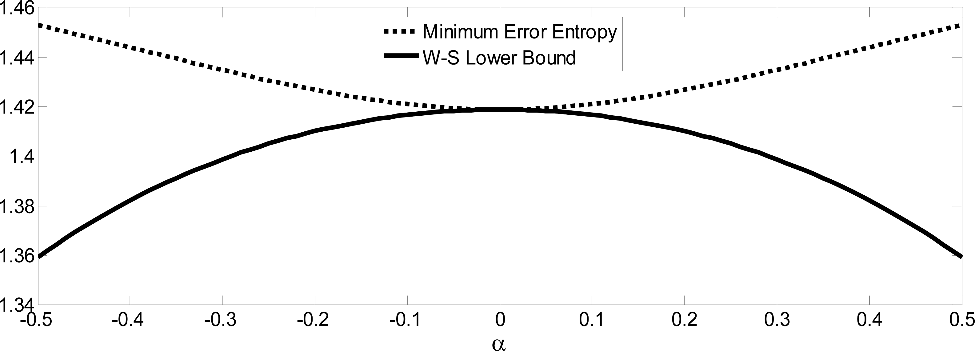
Remark: If X and Y are joint Gaussian, the MEE estimator of X based on Y will achieve the W-S lower bound. However, it should be noted that for most cases, the MEE estimator cannot achieve this performance bound. A simple example is given below.
Example 1: Consider the joint PDF pXY(x, y) = pX|Y (x|y)pY(y), where:
3. Characterization of the Gaussian Distribution
The W-S lower bound can be applied to characterize the Gaussian distribution, i.e., constructing some conditions under which a distribution is Gaussian (or joint Gaussian). The problem of characterization of the Gaussian distribution is an interesting problem, which has been extensively studied in the literature [23–27]. First, we introduce a lemma.
Lemma 1 [24]: Let X and Y be two random vectors, X ∈ ℝp, Y ∈ ℝ q. If X ∼(μX, ΣXX), and the distribution of Y given X is a q -dimensional Gaussian distribution with mean vector a + BX(a ∈ ℝq, B ∈ ℝ q×p), and constant covariance matrix Σ0 ∈ ℝq×q, then the joint distribution of will be a (p + q)-dimensional Gaussian distribution, whose mean vector and covariance matrix are:
Based on Lemma 1, we can state the following theorem.
Theorem 6: Let X and Y be two random vectors, X ∈ ℝn, Y ∈ ℝm. Assume that Y ∼ (μY, ΣYY), and the distribution of X given Y is a n -dimensional Gaussian distribution. If there exists a linear estimator X̂ = BY such that the error entropy H(E) achieves the W-S lower bound H (X|Y), where B∈ ℝ n×m, E = X−BY, then will be a (n + m)-dimensional multivariate Gaussian random vector.
Proof: Since the linear estimator X̂ = BY achieves the W-S lower bound, by Theorem 1, we have:
The next lemma is needed in the proof of Theorem 7.
Lemma 2 [25]: Let X ∈ ℝn and Y ∈ ℝm be two random vectors. Suppose the conditional densities pX|Y (x|y) and pY|X (y|x) are both (multivariate) Gaussian. Denote the covariance matrix of the conditional density pX|Y (x|y) by ΣX|Y (y). Then the following two statements are equivalent:
- (i)
the joint density function pXY (x,y) is multivariate Gaussian;
- (ii)
ΣX|Y(y) is constant on ℝm.
Theorem 7: Let X ∈ ℝn and Y ∈ ℝm be two random vectors. Suppose the conditional densities are pX|Y (x|y) and pY|X (y|x) both (multivariate) Gaussian. If the MEE estimator of X based on Y achieves the W-S lower bound H(X|Y), then the joint density function pXY (x,y) will be multivariate Gaussian.
Proof: Since the MEE estimator of X based on Y achieves the W-S lower bound, by Theorem 2, the conditional covariance matrix Σ X|Y (y) will not depend on y (i.e., be constant on ℝm). By Lemma 2, the joint density pXY will be multivariate Gaussian.
Before presenting Theorem 8, we introduce the third lemma, which is an extended version of Ghurye and Olkin’s theorem [23,26].
Lemma 3 [26]: Let U1 ∈ ℝp and U2 ∈ ℝq be two independent non-degenerate random vectors, and let X1 ∈ ℝp and X2 ∈ ℝq be two independent random vectors such that:
- (i)
is nonsingular,
- (ii)
none of the rows of and Γ2 = P−1C1 are null vectors.
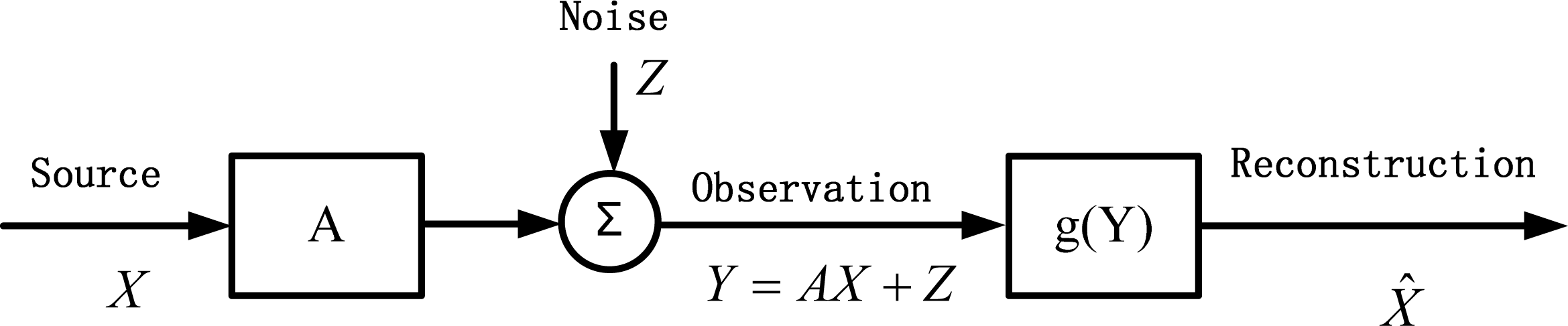
Consider now the problem of estimating the source X ∈ ℝn given the observation Y = AX + Z, where Y ∈ ℝm, A ∈ ℝm×n, and Z ∈ ℝm is the additive noise that is independent of X, as shown in Figure 2.
For the above estimation problem, the following theorem holds:
Theorem 8: For the estimation problem in Figure 2, if there exists a linear estimator X̂ = BY such that the error entrpy H(E) achieves the W-S lower bound H(X|Y), where B ∈ ℝ n×m, E = X − BY, then X and Z are multivariate Gaussian random vectors if the following conditions on A and B are satisfied:
- (i)
the matrices In −BA and Im + A(In −BA)−1B are nonsingular, where In and Im are identity matrices of order n and m respectively,
- (ii)
none of the rows of (In − BA)−1B and [Im + A(In −BA)−1B]−1A are null vectors.
Proof: Since Y = AX + Z, the error E can be expressed as:
Corollary 2: For the estimation problem in Figure 2, if X, Y, Z are all scalar random variables (m = n =1), and there exists a linear estimator X̂ = BY such that the error entropy H (E) achieves the W-S lower bound H (X|Y), where B ∈ ℝ, E = X − BY, then X and Z are scalar Gaussian random variables if A ≠ 0, B ≠ 0, and B ≠ 1/ A.
Remark: It is worth noting that when the condition that A ≠ 0, B ≠ 0, and B ≠ 1/A does not hold, some of the variables in the estimating system will become degenerate random variables. Specifically, when A = 0, the variable AX will be a degenerate random variable; when B = 0, the estimator X̂ = BY will become a degenerate random variable; when B=1/A(A ≠ 0), the variable (1−BA)X will be a degenerate random variable.
4. Conclusions
MEE estimation provides an appealing approach to design optimal estimators in the framework of information theory. Recent successful applications of the MEE criterion in the areas of signal processing and machine learning suggest that this estimation method has significant potential advantages over traditional MMSE estimation, especially when data possess non-Gaussian distributions. Though it has shown remarkable success in many applications, some theoretical aspects of the MEE estimation need further study. In this work, we reexamine the W-S lower bound on the MEE estimation, which is a Shannon theory-type performance bound on the estimation error entropy. We present some basic properties of the W-S lower bound, and give some interesting results on the characterization of Gaussian distribution using this performance bound. It is hoped that the results of this work will help us to gain insights into the attainment of the W-S lower bound in MEE estimation.
Acknowledgments
This work was supported by National Natural Science Foundation of China (No. 61372152, No. 90920301) and 973 Program (No. 2012CB316400, No. 2012CB316402).
Conflicts of Interest
The authors declare no conflict of interest.
References
- Kailath, T.; Sayed, A.H.; Hassibi, B. Linear Estimation; Prentice Hall: Upper Saddle River, NJ, USA, 2000. [Google Scholar]
- Weidemann, H.L.; Stear, E.B. Entropy analysis of estimating systems. IEEE T. Inform. Theory 1970, 16, 264–270. [Google Scholar]
- Tomita, Y.; Ohmatsu, S.; Soeda, T. An application of the information theory to estimation problems. Inform. Contr 1976, 32, 101–111. [Google Scholar]
- Kalata, P.; Priemer, R. Linear prediction, filtering and smoothing: An information theoretic approach. Inform. Sci 1979, 17, 1–14. [Google Scholar]
- Minamide, N. An extension of the entropy theorem for parameter estimation. Inform. Contr 1982, 53, 81–90. [Google Scholar]
- Janzura, M.; Koski, T.; Otahal, A. Minimum entropy of error principle in estimation. Inform. Sci 1994, 79, 123–144. [Google Scholar]
- Wolsztynski, E.; Thierry, E.; Pronzato, L. Minimum-entropy estimation in semi-parametric models. Signal Process 2005, 85, 937–949. [Google Scholar]
- Principe, J.C. Information Theoretic Learning: Renyi’s Entropy and Kernel Perspectives; Springer: New York, NY, USA, 2010. [Google Scholar]
- Chen, B.; Zhu, Y.; Hu, J.; Principe, J.C. System Parameter Identification: Information Criteria and Algorithms; Elsevier Inc: London, UK, 2013. [Google Scholar]
- Cover, T.M.; Thomas, J.A. Element of Information Theory; Wiley & Sons Inc.: New York, NY, USA, 1991. [Google Scholar]
- Otahal, A. Minimum entropy of error estimate for multi-dimensional parameter and finite-state-space observations. Kybernetika 1995, 31, 331–335. [Google Scholar]
- Chen, T.-L.; Geman, S. On the minimum entropy of a mixture of unimodal and symmetric distributions. IEEE Trans. Inform. Theory 2008, 54, 3166–3174. [Google Scholar]
- Chen, B.; Zhu, Y.; Hu, J.; Zhang, M. On optimal estimations with minimum error entropy criterion. J. Franklin Inst 2010, 347, 545–558. [Google Scholar]
- Chen, B.; Zhu, Y.; Hu, J.; Zhang, M. A new interpretation on the MMSE as a robust MEE criterion. Signal Process 2010, 90, 3313–3316. [Google Scholar]
- Chen, B.; Principe, J.C. Some further results on the minimum error entropy estimation. Entropy 2012, 14, 966–977. [Google Scholar]
- Chen, B.; Principe, J.C. On the smoothed minimum error entropy criterion. Entropy 2012, 14, 2311–2323. [Google Scholar]
- Erdogmus, D.; Principe, J.C. An error-entropy minimization algorithm for supervised training of nonlinear adaptive systems. IEEE Trans. Signal Process 2002, 50, 1780–1786. [Google Scholar]
- Erdogmus, D.; Principe, J.C. Generalized information potential criterion for adaptive system training. IEEE Trans. Neural Network 2002, 13, 1035–1044. [Google Scholar]
- Erdogmus, D.; Principe, J.C. Convergence properties and data efficiency of the minimum error entropy criterion in Adaline training. IEEE Trans. Signal Process 2003, 51, 1966–1978. [Google Scholar]
- Erdogmus, D.; Principe, J.C. From linear adaptive filtering to nonlinear information processing—The design and analysis of information processing systems. IEEE Signal Process. Mag 2006, 23, 14–33. [Google Scholar]
- Santamaria, I.; Erdogmus, D.; Principe, J.C. Entropy minimization for supervised digital communications channel equalization. IEEE Trans. Signal Process 2002, 50, 1184–1192. [Google Scholar]
- Chen, B.; Hu, J.; Pu, L.; Sun, Z. Stochastic gradient algorithm under (h, ϕ)-entropy criterion. Circuits Syst. Signal Process 2007, 26, 941–960. [Google Scholar]
- Ghurye, S.G.; Olkin, I. A characterization of the multivariate normal distribution. Ann. Math. Stat 1962, 33, 533–541. [Google Scholar]
- Fidalgo, J.L.; Albajar, R.A. Characterizing the general multivariate normal distribution through the conditional distributions. Extr. Math 1997, 12, 15–18. [Google Scholar]
- Bischoff, W.; Fieger, W. Characterization of the multivariate normal distribution by conditional normal distributions. Metrika 1991, 38, 239–248. [Google Scholar]
- Fisk, P.R. A note on a characterization of the multivariate normal distribution. Ann. Math. Stat 1970, 41, 486–494. [Google Scholar]
- Hamedani, G.G. On a recent characterization of the bivariate normal distribution. Metrika 1991, 38, 255–258. [Google Scholar]


© 2014 by the authors; licensee MDPI, Basel, Switzerland This article is an open access article distributed under the terms and conditions of the Creative Commons Attribution license (http://creativecommons.org/licenses/by/3.0/).
Share and Cite
Chen, B.; Wang, G.; Zheng, N.; Principe, J.C. A Note on the W-S Lower Bound of the MEE Estimation. Entropy 2014, 16, 814-824. https://doi.org/10.3390/e16020814
Chen B, Wang G, Zheng N, Principe JC. A Note on the W-S Lower Bound of the MEE Estimation. Entropy. 2014; 16(2):814-824. https://doi.org/10.3390/e16020814
Chicago/Turabian StyleChen, Badong, Guangmin Wang, Nanning Zheng, and Jose C. Principe. 2014. "A Note on the W-S Lower Bound of the MEE Estimation" Entropy 16, no. 2: 814-824. https://doi.org/10.3390/e16020814